An Improved Algorithm for Materialized View Selection

(1)

An Improved Algorithm for Materialized View

Selection

Lijuan Zhou

Information Engineering College, Capital Normal University, Beijing, 100037, China [email protected]

Haijun Geng

Mingsheng Xu

Abstract—The data warehouse is subject oriented, integrated, nonvolatile and time-varying data sets, which is used to support management decision-making. A data warehouse stores materialized views of data from one or more sources, with the purpose of efficiently implementing Decision-support or OLAP queries. One of the most important decisions in designing a data warehouse is the selection of materialized views to be maintained at the warehouse.The materialization of all views is not possible because of the space constraint and maintenance cost constraint.Selecting a suitable set of views that minimize the total cost associated with the materialized views is the key objective of data warehousing.

In this paper, first the query cost view selection problem model is proposed. Second, the methods for selecting materialized views are presented. The genetic algorithm is applied to the materialized view selection problem. But with the development of genetic process, the legal solution produced become more and more difficult. Therefore, improved algorithm has been presented in this paper. Finally, in order to test the function and efficiency of our algorithms, experiment simulation is adopted. The experiments show that the given methods can provide near-optimal solutions in limited time and work well in practical cases. Randomized algorithms will become invaluable tools for data warehouse evolution.

Index Terms—data warehouse; materialized view selection; genetic algorithm; ant colony algorithm; simulated annealing algorithm

I. INTRODUCTION

A materialized view is a pre-computed data summary that transparently allows users to query large amounts of data much more quickly than they could access the original data[1]. This summary is stored in a table so that users can query it directly. The materialized view is like a cache — a copy of the data that can be accessed quickly. This speed difference can be critical in applications where the query rate is high and the materialized views are complex, for example, aggregate queries over large

volumes of data[2].

One of the most common uses of materialized views is summary tables, materialized aggregate views. Data warehouses store large volumes of transaction history (fact tables) which are almost always queried using dimension grouping[3]. For example, in a retail database, sales transaction history can be queried by region, by item-category and month, or by year and store-id. Performing these queries from sales data in a reasonable time is almost impossible. To overcome the performance problem, users can define summary tables on the fact table and use these summary tables to perform faster queries.

In a typical organization, the information is stored in the form of multiple, independent, and heterogeneous data sources. Functioning as a “data library”, a data warehouse makes information readily available for querying and analysis. In essence, a data warehouse extracts, integrates, and stores “relevant” information from independent information sources into a central database. The information is stored at the warehouse in advance of the queries. In such a system, user queries can be answered using the information stored at the warehouse and need not be translated and shipped to the original source(s) for execution. Also, warehouse data is available for queries even when the original information source(s) are inaccessible due to real-time operations or updates.

(2)

set of views to materialize for answering queries, this was denoted view-selection problem (VSP).

Materialized views need corresponding storage space. User’s queries make use of materialized view and valuation query leads to query cost. Changes of source relationship leads to the materialize view update, which brings up materialized view maintenance cost. Most of all, the decrement of all cost can attain not only through query optimization and materialized view refresh, but also it can attain through selecting materialized view stored in data warehouse[4].Three factors must be considered when selecting materialized view: query cost, maintenance cost and spatial cost. In the article, we consider the view selection problem of selecting views to materialize in order to minimize the total maintenance cost under the constraint of a given query response time. We refer to this problem as the query cost view selection problem (QC_VSP).

It has been proven that the view selection problem is NP problem[5] [17]. To these complex combined and optimal questions, the time complexity and space complexity of the complete search algorithm become unacceptable. Sometimes the heuristic algorithm is not general, so the random algorithm is an effective and general solution. According to the statistic conception, the random algorithm produces bigger search space randomly and uses an evaluative function to make the search process approach to the expected goal gradually[14][15]. The random algorithm may find a reasonable and approximate optimization solution in a relative short time.

The algorithms of materialized view selection have greedy algorithm, genetic algorithm, ant colony algorithm and so on. These algorithms mainly consider the storage constraints, selecting a group of materialized views to make the sum of query cost and maintenance cost least. It is meaningful to select a set of materialized views under storage constraints in the case of disk space is tight. But with the cost of the disk greatly reduced and allows to storage large number of data, space restrictions is no longer a major constraints. Therefore, this article focuses on the question: under some certain conditions of query cost, selecting a set of materialized views to make the maintenance cost is minimal.

We give three algorithms to deal with QC_VSP. We do demonstrate the power of our approach with our experiment.

II. RELATED WORK

The problem of finding views to materialize to answer queries has traditionally been studied under the name of view selection. Its original motivation comes up in the context of data warehousing.

Harinarayan et al. [6] presented a greedy algorithm for the selection of materialized views so that query evaluation costs can be optimized in the special case of “data cubes”. However, the costs for view maintenance and storage were not addressed in this piece of work. Yang et al. [7] proposed a heuristic algorithm which utilizes a Multiple View Processing Plan (MVPP) to

obtain an optimal materialized view selection, such that the best combination of good performance and low maintenance cost can be achieved. However, this algorithm did not consider the system storage constraints.

Himanshu Gupta and Inderpal Singh Mumick [8] developed algorithms to select a set of views to materialize in a data warehouse in order to minimize the total query response time under the constraint of a given total view maintenance time. They have designed approximation algorithms for the special case of OR view graphs. Chuan Zhang and Jian Yang [9] proposed a completely different approach, Genetic Algorithm, to choose materialized views and demonstrate that it is practical and effective compared with heuristic approaches. Sanjay Agrawal, et al [10]. proposed an end-to-end solution to the problem of selecting materialized views and indexes. Their solution was implemented as part of a tuning wizard that ships with Microsoft SQL Server 2000.

Amit Shukla et al. [11]proposed a simple and fast heuristic algorithm, PBS, to select aggregates for precipitation. PBS runs several orders of magnitude faster than BPUS, and is fast enough to make the exploration of the time-space tradeoff feasible during system configuration.

Panos Kalnis et al. [12] proposed the application of

randomized search heuristics, namely Iterative Improvement and Simulated Annealing, which select fast

a sub-optimal set of views. The proposed method provided near-optimal solutions in limited time, being robust to data and query skew.

III. THE VIEW SELECTION COST GRAPH AND MODEL VSP aims to select a group of materialized views to satisfy one or more designing object. Designing object may make the cost function attain minimized value or can satisfy some restricted conditions. Obviously, if we make all user’s and system restricts satisfied, which may result to unfeasible programme. So, the selection of designing is an important factor which affects the quality of data warehouse.

Our problem in this paper can be described as follows: based on multiple queries, select a set of views to be materialized in order to make the total maintenance cost minimal under the constraint of a given query cost (QC_VSP)[18].

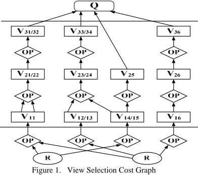
In order to solve QC_VSP, we define and construct View Selection Cost Graph (VSCG) as follows.

Definition 1: In the VSCG, each basic relation table creates a leaf node (resource table), R typification, there is a update frequency on the leaf node; the relation that is created through operation by some nodes is view nodes, V typification; the operation between nodes consist of a operation node, OP typification, each operation node is linked with a cost; the result is root, Q typification, which responds to a query.

(3)

each view node, view nodes can be defined as follows: if some a view’s location is number i node which begins from source table on a path(that is, the node is the number i created by source table on the path),assuming path j(studying for a serial number),the view name is Vij. If the node is the number k on the path l simultaneously, so we define the node name Vkl again, and store the relation Vij = Vkl, Figure 1 is a VSCG.

Figure 1. View Selection Cost Graph

In order to carry out the storage and computation of view effectively, in accordance with the above VSCG structure, view-node-matrix (VNM) is defined as follows.

Definition 3: Between the source relationship and query collection, there is a reasonable path and a large view nodes to compose of view node matrix, the number of rows of the matrix represent the largest number of view nodes in the entire path, the matrix column number represent the path number between the source relationship and query collection. The values of the matrix are three: if a certain view is materialized, Vij = 1; if they were not materialized, Vij = 0; if Vij was empty node, Vij =- 1.

For example, for Figure 1, the view nodes are composed of 3 rows 6 column matrix, in the matrix not each node is effective (with some empty nodes). Assume that view nodes V21, V31, V33, V25 were materialized, the view node matrix is:

0 0 0 0 0 0 1 1 0 0 1 0 1 1 1 1 1 0

⎡ ⎤

⎢ ⎥

⎢ − ⎥

⎣ ⎦

We give some definition to solve QC_VSP above. Below we will give a general description of QC_VSP in this paper: for a group of sources relationship and a group of queries in its definition, given a VSCG graphic and required, in a corresponding space conditions, select a group of materialized view M, which is subset of nodes in VSCG, in the restrictions that query processing costs using M does not exceed a given value of the user, making the total view maintenance cost smallest.

We can see the QC_VSP mainly related to the two costs: query processing cost and view maintenance cost. Its definition is as follows.

Definition 4: For a result set, the total query processing cost QV = Σi (si * QVi). Where si is the query frequency of view. QVi is the operation cost of view i in the course

of produce results set. Different views have different costs; the total query processing cost is expressed as the sum of all processing costs in operation from a table and materialized views as a starting point to the result set as an end point.

For the maintenance cost, in view of different views, because of its different operations, as it is taken as materialized view, the maintenance cost is different. Maintenance costs are also dependent on using incremental maintenance strategy or re-calculated strategy. In this paper, we use incremental maintenance, when the source relationship changes, only calculated the changes that occurred in view, that is, calculate data in the incremental change, and then it spread such changes to materialized view.

Definition 5: As for the view, when we take them as materialized view, the definition of total maintenance costs: MV = Σ i (fi *MVi), of which: view MVi is representative of the average cost when materialized view i updated, fi represents changes transmission frequencies from update of the source relationship reflected to materialized view i.

According to the above definition and calculation methods of query processing costs and the maintaining cost, below we give structure definition of each node in matrix of materialized view in definition 3.

Definition 6: the structure of each node in materialized view nodes matrix contains the following attributes:

(1) Node code. Node code identified only one view, because a certain materialized view may be a number of paths, there are some nodes having the same code in the matrix.

(2) Maintenance costs. Maintenance costs[13]here represent incremental maintenance costs of this view; when we take this view into materialized view, its maintenance cost is the maintenance cost multiplied by the frequency of maintenance.

(3) Maintenance frequency. When the view changes into the materialized view, the maintenance frequency represents the update frequency that the changes of source table reflected in the materialized view.

(4) Node value. Since this matrix has stored all possibility route information of problem view sets, but the length of every route may be not completely identical ,so this problem can not indicate a entire matrix, we use empty node to add to this matrix , while the route length does not reach i (the maximal route length), we assume that the first row of matrix is the route starting point , with the route stretching , the number of matrix rows increase ,when it get to the end of route, under the current matrix column, using empty space node to make up the remaining row. When initialing, we use -1 to represent the empty node; 0 represents view.

(5) Query cost. The operation costs of having this view represent the query costs of this view while this view has not materialized. When calculating the total query cost, this view query cost needs to multiply by its query frequency.

(4)

(7) Space cost. The space cost occupied by the view when the view has not materialized.

In the following, we give the cost model of QC_VSP. R={R1, …, Rn } : a set of source relations

Q={ Q1, …, Qn } : a set of queries s1, …, sm : query frequencies

f1, …, fn: source relation change propagation frequencies

QVi : the cost of answering a query

MVi : the cost of maintaining a materialized view QV=Σi( si*QVi) : the total cost of answering queries MV=Σi (fi*MVi): the total cost of maintaining materialized views.

QC_VSP is to select a set of views in order to minimize the total cost of maintaining materialized views under a given the total cost of answering queries.

Next we give the establishment method of QC_VSP model:

Import: (1) results sets. (2) source form.

(3) the given query processing costs Output:

(1) materialized view sets. (2) maintenance cost. (3) space cost Steps:

(1) Building a legitimate view as much as possible in the source form and the result sets. And providing the greatest number of paths possibly. Constructing VSCG according to definition 1.

(2) Using operation connect to the view and the view and form. That operation cost QV is to query cost.

(3)According to different route and the view number of each route, the footnote is labeled in all views of the whole model according to definition 2's method. And giving the view node matrix of entire model according to definition 3's method.

(4) Storing all operation costs of "operation OP".

(5) According to the principle of increment maintenance cost, calculating its maintenance cost while one node is taken as materialized view. Storing maintenance cost of all nodes.

(6) According to view selection algorithm, under the user query processing cost constraints, select a group of materialized view to make Σ i (fi * MVi) minimum, and output its value and its materialized view sets.

III. REALIZATION OF MATERIALIZED VIEWS SELECTION So as to QC_VSP, this paper gives three kinds of algorithm and realization. As follows: genetic algorithm (GA_VSP), dynamic integration of genetic algorithm and simulated annealing algorithm (GASAA_VSP) and dynamic integration of genetic algorithm and colony algorithm (GAACA_VSP).Below we make respective introductions.

A. Applying genetic algorithm to QC_VSP

It has been proved that the view selection problem is NP problem. Genetic Algorithm (GA) [20] is a

well-known approach to solve NP problem. Therefore the solution to QC_VSP applying for genetic algorithm (GA_VSP).

Based on the above cost model, we provide details on how to apply GA to QC_VSP.

1. The representation of the solution

Representation is a key issue in GA. We elaborate on a suitable representation of the solution. GA are working on binary encoded individuals, and the bits are often referred to as alleles. We first encode the solution of QC_VSP in chromosome presentation. The algorithm requires a mapping from VNM to a coded representation of the problem. Each chromosome is consisted of constant number of binary string, where the constant number is the number of the candidate views in VNM. The string 0 denotes the corresponding view is not materialized in the data warehouse. The string 1 denotes the corresponding view is materialized in the data warehouse. For example, given a VNM that consisted of 8 candidate views, the solution of the problem should be converted into a binary string [1 0 0 1 0 1 0 0], this means the 1st, the 4th; the 6th corresponding views have been materialized[16].

2. The initial population

The initial population will be a pool of randomly generated binary strings of size n.

3. Fitness function

The fitness function measures how good a solution is by providing a fitness value as follows: if the fitness is high, the solution satisfies the goal; if the fitness is low, the genome should be discarded. Since the objective in our cost model is stated as the minimization of maintenance cost and the fitness function of GA is naturally stated as maximization, there should be a transformation from our cost function to the fitness function. Thus, the fitness function can be defined as follows:

F(x)=C/f(x)

Here C may be taken as an input coefficient. f(x) denoted the total cost function of maintaining materialized views. F(x) is the fitness function.

With this transformation, we can reach our goal. The less the cost function become, the more the fitness functions become.

4. Genetic operators

We introduce the genetic operators including selection, crossover and mutation in QC_VSP.

(1) Selection

The selection is a process in which individuals are reproduced according to their fitness. Individuals with higher fitness values have higher chance to survive. There are many well-known kind of selection such as random selection, ranking selection etc. We adopt the popular roulette wheel method as our selection operator.

(2) Crossover

The crossover operator attempts to swap partially good solutions in order to get better results. The crossover operator enables us to define new starting points for a search. We use one-point crossover in our experiment.

(5)

0 1 1 1 0 0 1 1

1 0 1 0 1 1 0 0

⎡ ⎤

⎣ ⎦

⎡ ⎤

⎣ ⎦

Where the symbol represents the position of crossover applied. The results of crossover are:

0 1 1 0 1 1 0 0 1 0 1 1 0 0 1 1

⎡ ⎤

⎣ ⎦

⎡ ⎤

⎣ ⎦

(3) Mutation

The mutation operator is a means of the occasional random alteration of the value of a string position. It introduces new features that may not present in any member of the population. The mutation is performed on a gene by gene basic.

For example, assume that the 4th bit in the individual is selected for mutation:

Individual: [1 0 0 1 1 0 0 1] Individual after mutation: [1 0 0 0 1 0 0 1] The main aim of an adequate genetic operator is to keep the search goal-oriented and also to maintain the diversity of the population.

5. Termination

The terminated conditions of genetic algorithm: genetic algorithm’s terminated conditions are actually genetic algorithm and ant colony algorithm best integration of time. We set the maximum number of iterations of the genetic Gmax, the smallest evolutionary

rate Gminratio .

In the experiment which aims to solve QC_VSP applying for genetic algorithm, with the development of genetic process, the legal solution produced become more and more difficult, so a lot of solutions are eliminated and producing time of the solutions is lengthened, which adds difficulty to the solution in GA_VSP algorithm. Therefore, two improved algorithms have been presented, which are the combination of simulated annealing algorithm and genetic algorithm and it is called GASAA_VSP algorithm and the combination of genetic algorithm and ant colony algorithm and it is called GAACA_VSP algorithm.

B. Applying dynamic integration of simulated annealing algorithm and genetic algorithm to QC_VSP

In GASAA_VSP, we get a group of results applying for genetic algorithm; we can confirm organization researching could get on in way of population. At the same time, this way may research several regions in result space and makes some communications each other. Simulated annealing algorithm [21]could be used to judge result correctness, according to the acceptance rule in simulated annealing algorithm, the algorithm can accept not only optimization results but also deterioration results. At the beginning, the algorithm may accept the poorer deterioration results, with the annealing, can only accept the better deterioration results, finally, would not accept any deterioration results. This will not only expand the choosing scope of results, and ensure the diversity of solutions, but also may cause algorithm jumping out from local optimum; it is more likely to find the whole optimal solution, while ensuring the convergence algorithm[19].

The simulated annealing algorithm starts from one initialized solution and gets relative optimization solution of combined optimization problem that is given control parameter value after a great deal solutions’ changes. Then the value of control parameter t is reduced and Metropolis algorithm is operated repeatedly, we can get whole optimization solution of combined optimization problem finally. The simulated annealing algorithm uses Metropolis algorithm to produce the sequence of combined optimization problem solution and decides whether it accepts the transferring from the current solution i to new solution j by the transferring probability Pt corresponding Metropolis rule.

( ) ( ) ( ) ( )

1,

( )

exp

t

f i f j

P i j F i f i

otherwise t

≤ ⎧

⎪

⇒ =⎨ ⎡ − ⎤

⎢ ⎥

⎪

⎣ ⎦

⎩

In the equation above, t R+ expresses control parameter. First t is set the bigger value (corresponding to dissolution temperature of solid), after performing enough transfer to reduce value of t (corresponding to reduce temperature gradually), the process is repeated again and again until it meet some stopping rule to end the algorithm.

The GASAA_VSP algorithm accepts the new solution according to the Metropolis rule, so it can accept the worsen solution in a limited range except the optimization solution. Firstly the value t is big, so it may accept the worst solution. When the value t reduces, it only accepts the worse solution. Finally, it doesn’t accept any bad solution when the value t closes to zero. This makes the algorithm not only jump from local optimization, but also gain the whole optimization solution of combined optimization problem, and it is simple and general.

In the course of the simulated annealing performing, the probability of the algorithm which returns some whole optimization solution augments monotonously with the control parameter t is reduced.

The basic idea of GASAA_VSP algorithm which combines the simulated algorithm with the genetic algorithm to solve QC_VSP is: to start from the select original solution, reduce the value of the control parameter t and use the genetic algorithm to produce new solution. Then it uses acceptable rule to perform repeatedly the course of “produce new solution----calculate goal function errand----judge whether accept new solution----accept (or give up) new solution”. The following is details of GASAA_VSP algorithm:

(1)Solution space:

The solution space is limited in all feasible solution under the given the query cost:

S= {(V1, …, Vn) ︳QV<=E, Vi∈{0,1} }

The view is materialized when Vi equals to 1; the view

isn’t materialized when Vi equals to 0.

(2)The goal function:

The goal function of QC_VSP is the minimal total maintenance cost. The restriction condition is given total query cost.

(6)

New solution is produced by the genetic operators including selection, crossover and mutation.

The selection is a process in which individuals are reproduced according to their fitness. We adopt the popular roulette wheel method as our selection operator.

We use one-point crossover. The mutation is performed on a gene by gene basic.

(4) Goal function errand:

Goal function is the view maintenance cost in this paper. According to the new solution we calculate the view maintenance cost errand:

⊿f=Max(parent->mprice)-Child1->mprice

⊿f is the goal function errand between the current solution and new solution that is subtracting the generation maintenance from the maximal elder maintenance cost.

We need to gain maintenance cost of the new solution to judge the solution feasibility and see whether it meets the given query cost.

(5)Acceptance rule:

The following is acceptance rule.

0 (when query cost is more than given value)

1 and 0

( / )otherwise QV E

P QV E f

Exp f t

> ⎧

⎪

=_⎨ ≤ ∆ >

⎪ _∆

⎩

When new solution is accepted, it is replaced by current solution.

The simulated annealing algorithm can extend the solution selection space, keep the solution multiform and reduce the difficulty of producing solution. At the same time with the genetic algorithm producing new solution, it assures the steady descendible of group characteristic. The GASAA_VSP algorithm may accept not only optimization but the worse solution in some range following the annealing and genetic course synchronously. It can accept that the probability of worse solution approach to zero, make the algorithm jump from local optimization, find the whole optimization solution and assure solution converge slowly.

We make use of the advantage of combining the genetic algorithm with the simulated annealing algorithm and solve QC_VSP problem in the paper. The GASAA_VSP algorithm proposed can produce better. The experiment results show this.

C. Applying integration of ant colony algorithm and genetic algorithm to QC_VSP

Ant Colony Optimization (ACO)[22] is a multi agent approach that simulates the foraging behavior of ants for solving difficult combinatorial optimization problems. Ants are social insects whose behavior is directed more towards the survival of colony as a whole than that of a single individual of the colony. An important and interesting behavior of an ant colony is its indirect co-operative foraging process. While walking from the food sources to the nest and vice versa, ants deposit a substance, called pheromone trail. Ants can smell pheromone; when choosing their way they tend to choose, with high probability, paths marked by strong pheromone

concentration (shorter path). Also, other ants can use pheromone to find the location of food sources found by their nest mates. Therefore, ACO simulates the optimization of ant foraging behavior[23].

Genetic algorithm has the ability of doing a global searching quickly and stochastically. But it can not make use of enough system output information. It has to do a large redundancy repeat for the result when solving to certain scope. So the efficiency to solve precision results is reduced. Ant algorithm converges on the optimization path through information pheromone accumulation an d renewa1. It has the ability of parallel processing an d global searching . The speed at which the ant algorithm gives the solution is slow. because there is little information pheromone on the path early. The algorithm in this paper is based on the combination of genetic algorithm and ant algorithm. First, it adopts genetic algorithm to give

information pheromone to distribute. Second, it makes use of the an t algorithm to give the precision of the solution. Finally, it develops enough advantage of the two algorithms[24].

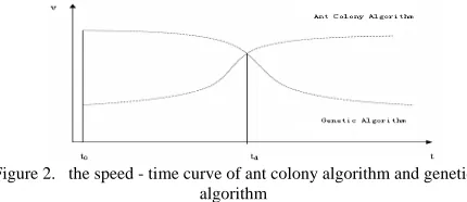
From the research of genetic algorithm and ant colony algorithm experiments show that their overall posture shown in Figure 2. As can be seen from the figure, the genetic algorithm has a high rate of convergence to the optimal solution in the period of to-td, but after td efficiency is significantly decreased. The ant colony algorithm search speed is low due to lack of information in the early stages of search (to-td), but with the accumulation of pheromone, the speed of convergence to the optimal solution rapidly increased. The idea of

Figure 2. the speed - time curve of ant colony algorithm and genetic algorithm

dynamic integration of Genetic algorithm and ant colony algorithm is that: before the combination point td we use genetic algorithm, after the fusion point we use ant colony algorithm. The dynamic integration strategy presented here can ensure that ant colony algorithm and genetic algorithm is integrated at the best time, specific methods are as follows:

(1) Set the maximum number of interations of genetic using Gmax.

(2) Within the limits the evolution rate is less than the minimum rate of Gminratio. So this time we can terminate

the genetic algorithm, and go to the ant algorithm. The ant colony algorithm rules in Materialized View Selection are as follows:

(1) The rule of pheromone update:

(7)

Local update formula is:

τ

_ijnew =

ρ τ

* _ijold + −(1

ρ τ

) * ₀ (1)

Where ρ is pheromone evaporation factor, 1-ρ is residual factor pheromone, in order to prevent the unlimited accumulation of information, ρ∈ [0,1), τ0 is the initial pheromone.

Global update formula is:

* (1 ) *

new old

ij ij ij

τ

=

ρ τ

+ −

ρ

∆

τ

₍₂₎

where △τij is the pheromone increment on this cycle

path (i, j), the initial moment of △τij = 0, △τij = 1/MV

(M), where MV (M) is maintenance cost of the optimal solution.

The formula of state transition rules:

( ) ( )

( ) ( ) 0,1

k k

ij j

pij

k k

ij j

k

α β

τ η

α β

τ η

⎡ ⎤ ⎡ ⎤

⎢ ⎥ ⎢ ⎥

⎣ ⎦ ⎣ ⎦

=

⎡ ⎤ ⎡ ⎤

∑ ⎢⎣ ⎥ ⎢⎦ ⎣ ⎥⎦ =

(3)

In the above formula k = 0 indicates that the view is not materialized, while k = 1 indicates that the view is materialized, in which ηj(k) is the local heuristic

information of Vj .it is defined as follows:

1

( )k ₍ _* _* ₎

j w_q QV_j w_m MV_j

η

= ₊ ₍₄₎

Where wq, wm is respectively the query cost and

maintenance cost normalization factor.

(2) The node Vi except the initial set of nodes and the query set nodes, each ant try to determine whether the each subsequent node Vj is materialized, it is mainly

based on the edge eij global heuristic information τij(k)

and node Vj local heuristic information to complete this

work.

When the ant enters the node Vj, it will be

synthetically consider the result of speculation of all predecessor nodes Vj, and hypothesize whether the node

Vj is materialized in this interactive. Ant k in accordance

with the following formula to guess whether Vj will be

materialized. Ant algorithm control parameter settings: α = β = 3, wq = 4, wm = 6, ρ = 0.3.

The formula of guessing probability:

which guess is materilized the number of precursors of node

the number of precursors of node

V_j V_j

p j

Vj

(k) =

(5)

(3) When one of the following conditions is met, the ant colony algorithms are terminated.

① Ant colony algorithm iterations reaches the maximum number of iterations Antmax.

② Offspring are less than optimal solution Antminratio,

Antmax = 70, Antminratio = 0.2%.

In the early stage we adopt genetic algorithm, later use ant colony algorithm, the integration of the two algorithms are very important, including the following issues.

①Dynamic integration time is when the genetic algorithm is terminated.

② The initial value of pheromone information of ant colony algorithm: Using the initial pheromone distribution accepts from the genetic algorithm, setting the initial pheromone information as follows:

( )

S

_k

C

_k

G

_k

ij

τ

=

τ

+

τ

₍₆₎

Where ( ) C _k ij τ

pheromone is constant, the number is 30, and τG kij( ) _{is the result from the genetic algorithm} converted to the pheromone information.

The method to convert the result from the genetic algorithm to the pheromone information is that:selecting top 5% of the individual as a genetic optimization solution set when the genetic algorithm is terminated,

( ) G k ij

τ =0 at the beginning, if a view is materialized, then the τG k_ij( ) plus 20.

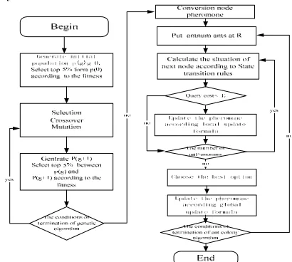
Figure 3. the algorithm of combination of ant colony algorithm and genetic algorithm

The algorithm of combination of ant colony algorithm and genetic algorithm is described in Figure 3.

IV.EXPERIMENT RESEARCH

In order to verify the validity of the algorithm, this paper carried out experimental simulation.

Experiments use Windows XP, use VC 6.0 to program, and use SQL Server 2000 as database. The goal is to make maintenance cost minimal under the query cost constraint.

(8)

5000, 2000, 800.The results shown as Table1,Table 2 ,Table 3 .

TABLE 1 THE RESULTS OF EXPERIMENT

The name of algorithm

The number of

views

Query cost

Maintain cost

GA_VSP ACA_VSP GASAA_VSP GAACA_VSP

103 124 130 154

4102.58 4265.86 4336.84 4433.57

689.22 653.64 630.48 600.56

The number of views

Query cost

Maintain Cost

184 215 243 286

1054.23 1345.62 1546.34 1676.64

1563.78 1463.45 1210.56 1005.45

The number

of views Query _cost Maintain _cost

513 534 564 604

654.23 700.24 740.35 780.58

3864.57 3765.54 3546.87 3102.45

From table1, table2, table3, we can draw the conclusion that as the increasing of the number of materialized views the GAACA_VSP show it’s superior.

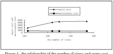
We can get the result showed in Figure 4 using the data in Table1.

From Figure 4 we can draw the following conclusions: (1) The query cost of four randomized algorithms is quite different, dynamic GASAA_VSP and GAACA_VSP are closest to the value of given, indicating a better performance. Ant colony algorithm’s query cost is closer to the value of given, but its maintenance cost is not very good.

(2) GAACA_VSP’s maintain cost is the best among the three algorithms.

0 1000 2000 3000 4000 5000

100 120 140 160

the number of views

query

cost and

mainte

nance cost

query cost maintenance cost

Figure 4. the relationship of the number of views and query cost ,maintenance cost

V. CONCLUSION

One of the most important decisions is to choose some views to materialize in the data warehouse design; the majority of studies have targeted disk space constraints,

but with the price of hard drive down, the disk space constraint have been not so much important. According to the practical application, especially in OLAP the main factor was not the space constraint, but the rapid response to user queries. Therefore, this paper presents under the query cost constraint to choose a group of views to materialize to make sure the maintain cost is least. Dynamic integration algorithm is present to solve the materialized view selection in this paper; the results show that the performance of dynamic integration algorithm is better than single use of genetic algorithm and ant colony algorithm, proving the feasibility and effectiveness of dynamic integration algorithm.

We solve the problem using two methods, one is GASAA_VSP, the other is GAACA_VSP, and both of them show good performance.

ACKNOWLEDGEMENTS

This work was supported by National Key Technology R&D Program (2009BADA9B02).

This work was supported by Beijing Educational Committee science and technology development plan project(KM200810028016), Capital Normal University project and Beijing Information project.

This work wassupported by the Open Project Program of Key Laboratory of Digital Agricultural Early-warning Technology, Ministry of Agriculture

,

Beijing, 100037.

VII.REFERENCES

[1] Ghoshal, A. and Vijay Kumar, T.V. ,Greedy Algorithms for Materialized Views Selection, In the proceedings of the International Conference on Data Management (ICDM-2009), Ghaziabad February 10-11, pp.101-113, 2009. [2] Tayi, G.K., Ballou, D.P., Examining Data Quality. In

Communications of the ACM, 41(2), pp. 54-57, 1998. [3] Chun Zhang, Xin Yao and Jian Yang,An Evolutionary

Approach to Materialize Views Selection in a Data Warehouse Environment. IEEE Trans. On Systems, Man and Cybernetics, Part C, SEPT. 2001, v31 (3).

[4] H. Gupta, I.S. Mumick, Selection of views to materialize under a maintenance cost constraint. In Proc.7th International Conference on Database Theory (ICDT'99), Jerusalem, Israel, pp. 453–470, 1999.

[5] D.Theodiratos, M.Bouzeghoub ,A General Framework for the View Selection Problem for Data Warehouse Design and Evolution.[c]Proceedings of the ACM third international workshop on Data Warehousing and OLAP. Nov.6-11, 2000.

[6] V. Harinarayan, A. Rajaraman, and J. Ullman, “Implementing data cubes efficiently”. Proceedings of ACM SIGMOD 1996 International Conference on Management of Data, Montreal, Canada, , pp. 205--216, 1996.

[7] J.Yang, K. Karlapalem, and Q. Li, “A framework for designing materialized views in data warehousing environment”. Proceedings of 17th IEEE International conference on Distributed Computing Systems, Maryland,

U.S.A., May 1997.

(9)

[9] J.T. Horng, Y.J.Chang,Materialized View Selection Using Genetic Algorithms in a Data Warehouse [c]. Proceedings of the 1999 Congress on Evolutionary Computation , pp. 1999,vol.3.

[10] S. Agrawal, S. Chaudhuri, and V. Narasayya, “Automated Selection of Materialized Views and Indexes in SQL Databases,” Proceedings of International Conference on Very Large Database Systems, 2000.

[11] A. Shukla, P. Deshpande, and J. F. Naughton, “Materialized view selection for multidimensional datasets,” in Proc. 24th Int. Conf. Very Large Data Bases, 1998, pp. 488–499.

[12]P. Kalnis, N. Mamoulis, and D. Papadias, “View Selection Using Randomized Search,” Data and Knowledge Eng., vol .42, no. 1, 2002.

[13]Serna-Encinas, M.T. and Hoya-Montano, J.A.: Algorithm for selection of materialized views: based on a costs model,In proceeding of eighth International conference on Current Trends in Computer Science, pp.18-24, 2007. [14] Satyanarayana R Valluri, Soujanya Vadapalli, and

Kamalakar Karlapalem,View Relevance Driven Materialized View Selection in data warehousing Environment. The Thirteenth ADC 2002, Melbourne, Australia. Vol.5.

[15]C. Zhang and J. Yang, “Genetic algorithm for materialized view selection in data warehouse environments,” Proceedings of the International Conference on Data Warehousing and Knowledge Discovery, LNCS, vol. 1676,pp. 116–125, 1999.

[16]D.Theodiratos,M.Bouzeghoub,A General Framework for the View Selection Problem for Data Warehouse Design and Evolution.[c]Proceedings of the ACM third international workshop on Data Warehousing and OLAP.Nov.6-11,2000,Mclean,VA USA.

[17]Rada Chirkova, Chen Li, Materializing Views with Minimal Size To Answer Queries. Proceedings of the twenty-second ACM SIGMOD-SIGACT-SIGART symposium. Principles of database systems,pp.38-48,2003. [18]Lijuan Zhou,Selecting materialized views in a data

warehouse.IS&T/SPIE’s 15th Annual Symposium, Storage and Retrieval for Media Databass Vol.5021, 2003,Jan. California,USA.

[19]Gupta, H., Harinarayan, V., Rajaraman, A., and Ullman, J.D., Index Selection for OLAP, 13th ICDE Conference, pp:208-219,April 1997.

[20]Kalnis P, Mamoulis N, Papadias D.View selection using randomized search[J]. search[J]. 2002,42(1),pp.89-111. [21]R. Derakhshan, F. Dehne, O. Korn and B. Stantic,

“Simulated Annealing for Materialized View Seletion in Data Warehousing Environment,”DBA, pp. 89-94,2006. [22]G. Wang, W. Gang and R.Kastner, “Application

Partitioning on programmable platforms using Ant Colony Optimization”, Journal of Embedded Computing, Vol.2, Issue 1, 2006

[23]Marco Dorigo,GambardeUa,Luca Maria.Ant colonies for the traveling salesman probl~n Biosystems, 43(2)：pp.73

～81,1997 .

[24]Marco Dorigo, GambardeUa, Luca Maria. Ant colony system: A cooperative learning approach to the traveling salesman problem. IEEE Trans On Evolutionary Computation,pp.53～66,1997.

LiJuan Zhou received the Btech degree in Computer Application Technology from the HeiLongJiang University in 1991, the MS degree in Computer Application Technology from the Harbin University of Science And Technology in 1998 and the PhD degree in Computer Application Technology from the Harbin Engineering University in 2004.