https://doi.org/10.5194/esd-9-507-2018
© Author(s) 2018. This work is distributed under the Creative Commons Attribution 4.0 License.
Analytically tractable climate–carbon cycle feedbacks
under 21st century anthropogenic forcing
Steven J. Lade1,2,3, Jonathan F. Donges1,4, Ingo Fetzer1,3, John M. Anderies5, Christian Beer3,6, Sarah E. Cornell1, Thomas Gasser7, Jon Norberg1, Katherine Richardson8, Johan Rockström1, and
Will Steffen1,2
1Stockholm Resilience Centre, Stockholm University, Stockholm, Sweden 2Fenner School of Environment and Society, The Australian National
University, Australian Capital Territory, Canberra, Australia
3Bolin Centre for Climate Research, Stockholm University, Stockholm, Sweden 4Potsdam Institute for Climate Impact Research, Potsdam, Germany 5School of Sustainability and School of Human Evolution and Social
Change, Arizona State University, Tempe, Arizona, USA
6Department of Environmental Science and Analytical Chemistry
(ACES), Stockholm University, Stockholm, Sweden
7International Institute for Applied Systems Analysis, Laxenburg, Austria 8Center for Macroecology, Evolution, and Climate, University of Copenhagen,
Natural History Museum of Denmark, Copenhagen, Denmark
Correspondence:Steven J. Lade ([email protected])
Received: 1 September 2017 – Discussion started: 12 September 2017 Revised: 23 April 2018 – Accepted: 27 April 2018 – Published: 17 May 2018
Abstract. Changes to climate–carbon cycle feedbacks may significantly affect the Earth system’s response to greenhouse gas emissions. These feedbacks are usually analysed from numerical output of complex and arguably opaque Earth system models. Here, we construct a stylised global climate–carbon cycle model, test its output against comprehensive Earth system models, and investigate the strengths of its climate–carbon cycle feedbacks analytically. The analytical expressions we obtain aid understanding of carbon cycle feedbacks and the operation of the carbon cycle. Specific results include that different feedback formalisms measure fundamentally the same climate–carbon cycle processes; temperature dependence of the solubility pump, biological pump, and CO2
solubility all contribute approximately equally to the ocean climate–carbon feedback; and concentration–carbon feedbacks may be more sensitive to future climate change than climate–carbon feedbacks. Simple models such as that developed here also provide “workbenches” for simple but mechanistically based explorations of Earth system processes, such as interactions and feedbacks between the planetary boundaries, that are currently too uncertain to be included in comprehensive Earth system models.
1 Introduction
The exchanges of carbon between the atmosphere and other components of the Earth system, collectively known as the carbon cycle, currently constitute important negative (damp-ening) feedbacks on the effect of anthropogenic carbon emis-sions on climate change. Carbon sinks in the land and the ocean each currently take up about one-quarter of
car-Climate change
Temperature, T
Land carbon
Total vegetation and soils, ct
Ocean carbon
Ocean mixed layer, cm (Total ocean, cM)
Atmosphere carbon, ca
R
adi
at
ive
forcing
-
-+
-
-+
+
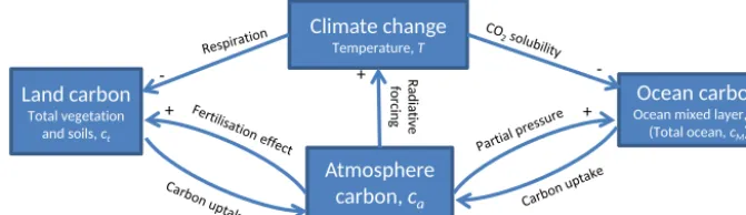
Figure 1.Climate–carbon cycle feedbacks and state variables as represented in the stylised model introduced in this paper. Carbon stored on land in vegetation and soils is aggregated into a single stockct. Ocean mixed layer carbon,cm, is the only explicitly modelled ocean stock of
carbon; though to estimate carbon cycle feedbacks we also calculate total ocean carbon (Eq. 7).
bon uptakes even under identical atmospheric concentration or emission scenarios (Joos et al., 2013).
Here, we develop a stylised model of the global carbon cycle and its role in the climate system to explore the poten-tial weakening of carbon cycle feedbacks on policy-relevant timescales (<100 years) up to the year 2100. Whereas com-prehensive Earth system models are generally used for pro-jections of climate, models of the Earth system of low com-plexity are useful for improving mechanistic understanding of Earth system processes and for enabling learning (Randers et al., 2016; Raupach, 2013). Compared to comprehensive Earth system models, our model has far fewer parameters, can be computed much more rapidly, can be more rapidly understood by both researchers and policymakers, and is even sufficiently simple that analytical results about feed-back strengths can be derived. Compared to previous stylised models (Gregory et al., 2009; Joos et al., 1996; Meinshausen et al., 2011a, c; Gasser et al., 2017a), our model features sim-ple mechanistic representations, as opposed to parametric fits to Earth system model output, of aggregated carbon uptake both on land and in the ocean. Our stylised and mechanisti-cally based climate–carbon cycle model also offers a work-bench for investigating the influence of mechanisms that are at present too uncertain, poorly defined, or computationally intensive to include in current Earth system models. Such stylised models are valuable for exploring the uncertain but potentially highly impactful Earth system dynamics such as interactions between climatic and social tipping elements (Lenton et al., 2008; Kriegler et al., 2009; Schellnhuber et al., 2016) and the planetary boundaries (Rockström et al., 2009; Steffen et al., 2015).
Analyses of climate–carbon cycle feedbacks convention-ally distinguish four different feedbacks (Fig. 1) (Friedling-stein, 2015; Ciais et al., 2013). (i) In the land concentration– carbon feedback, higher atmospheric carbon concentration generally leads to increased carbon uptake due to the fertili-sation effect, in which increased CO2stimulates primary
pro-ductivity. (ii) In the ocean concentration–carbon feedback, physical, chemical, and biological processes interact to sink carbon. Atmospheric CO2 dissolves and dissociates in the
upper layer of the ocean to then be transported deeper by physical and biological processes. The concentration–carbon feedbacks are generally negative, dampening the effects of anthropogenic emissions. (iii) In the land climate–carbon feedback, higher temperatures, along with other associated changes in climate, generally lead to decreased storage on land at the global scale, for example due to the increase in respiration rates with temperature. (iv) In the ocean climate– carbon feedback, higher temperatures generally lead to re-duced carbon uptake by the ocean, for example due to de-creasing solubility of CO2. The climate–carbon feedbacks
are generally positive, amplifying the effects of carbon emis-sions.
We begin by introducing our stylised carbon cycle model and testing its output against historical observations and fu-ture projections of Earth system models. Having thus estab-lished the model’s performance, we introduce different for-malisms used to quantify climate–carbon cycle feedbacks and describe how they can be computed both numerically and analytically from the model. We use our results to analyt-ically study the relative strengths of different climate–carbon cycle feedbacks and how they may change in the future, as well as to compare different feedback formalisms. We con-clude by speculating on how this stylised model could be used as a “workbench” for studying a range of complex Earth system processes, especially those related to the biosphere.
2 Model formulation
There is well-developed literature on stylised models used for gaining a deeper understanding of Earth system dynamics and even for successfully emulating the outputs of compre-hensive coupled atmosphere–ocean and carbon cycle mod-els (Anderies et al., 2013; Gregory et al., 2009; Joos et al., 1996; Meinshausen et al., 2011a, c; Gasser et al., 2017a). We developed a combination of existing models and new formu-lations to construct a global climate–carbon cycle model with the following characteristics.
policy-relevant timescale of the present to the year 2100. Stylised carbon cycle models often do not, for exam-ple, include explicit representations of the solubility or biological pumps.
2. The model produces quantitatively plausible output for carbon stocks and temperature changes.
3. All parameters have a direct biophysical or biogeo-chemical interpretation, although these parameters may be at an aggregated scale (for example, a parameter for the net global fertilisation effect, rather than leaf phys-iological parameters). We avoid models or model com-ponents constructed by purely parametric fits, such as impulse response functions, to historical data or projec-tions of Earth system models (Kamiuto, 1994; Gasser et al., 2017b; Joos et al., 1996; Harman et al., 2011; Gre-gory et al., 2009; Meinshausen et al., 2011a).
4. The model is sufficiently simple that calculation of the model’s feedback strengths is readily analytically tractable. This tractability may come at the expense of complexity, for example multiple terrestrial car-bon compartments, or accuracy at millennial or longer timescales (Lenton, 2000; Randers et al., 2016).
Building on the work of Anderies et al. (2013), we con-structed a simple model with globally aggregated stocks of atmospheric carbon in the form of carbon dioxide,ca;
terres-trial carbon, including vegetation and soil carbon,ct; and
dis-solved inorganic carbon (DIC) in the ocean mixed layer,cm.
The model’s fourth state variable is global mean surface tem-perature relative to pre-industrial,1T =T −T0. Compared
to Anderies et al. (2013), our model includes more realistic representation of terrestrial and ocean processes but without increase in model complexity, as well as time lags for climate response to CO2.
We now describe the dynamics of the land carbon stock, the ocean carbon stock, and atmospheric carbon and temper-ature in our model.
2.1 Land
Net primary production (NPP) is the net uptake of carbon from the atmosphere by plants through photosynthesis. NPP is expected to increase with concentration of atmospheric carbon dioxide ca. A simple parameterisation of this
so-called fertilisation effect is “Keeling’s formula” for global NPP (Bacastow et al., 1973; Alexandrov et al., 2003):
NPP(ca)=NPP0
1+KClog
ca
ca0
. (1)
Throughout this article, the subscript “0” denotes the value of the quantity at a pre-industrial equilibrium, and “log” de-notes natural logarithm. Keeling’s formula incorporates all
climate-change-related effects on global NPP occurring si-multaneously with carbon dioxide changes, for example, pre-cipitation and temperature effects, in addition to fertilisation effects. The curvature of the log function represents limita-tions to NPP such as changing carbon-use efficiency (Körner, 2003) or nutrient limitations (Zaehle et al., 2010). Constant climate sensitivity is also a key assumption, otherwise the relative weight of climate and CO2 effects on NPP would
change.
At the same time, carbon loss from the world’s soils through respiration, R, is expected to increase at higher global mean surface temperature,1T. We approximate the net temperature response of global soil respiration using the Q10 formalism R(1T)=R0Q1T /10R ct/ct0 (Xu and Shang,
2016), where QR is the proportional increase in
respira-tion for a 10 K temperature increase. We assume that pre-industrial soil respiration is balanced by pre-pre-industrial NPP, R0=NPP0. To avoid introducing multiple pools of carbon
into the model, we also have to assume that global soil respi-ration is proportional to total land carbon (rather than soil carbon). Respiration in our model also implicitly includes other carbon-emitting processes such as wildfires or insect disturbances.
It follows that the change in global terrestrial carbon stor-age is
dct
dt =NPP0
1+KClog
ca
ca0
−NPP0
ct0
Q1T /10R ct−LUC(t).
In this expression we have also included loss of terrestrial carbon due to land use emissions LUC(t). We rearrange this expression to give
dct
dt = NPP0
ct0
Q1T /10R [K(ca, 1T)−ct]−LUC(t), (2)
where the terrestrial carbon carrying capacity is
K(ca, 1T)=
1+KClogcca
a0
Q1T /10R
ct0. (3)
For model simplicity, we do not explicitly model fac-tors affecting terrestrial carbon uptake such as seasonality, species interactions, species functionality, migration, and re-gional variability.
2.2 Ocean
and biological pumps, and ocean–atmosphere diffusion on upper-ocean mixed layer carbon.
Ocean uptake of carbon dioxide from the atmosphere is chemically buffered by other species of DIC such as HCO−3 and CO23−, which are produced when dissolved CO2reacts
with water. The reaction of CO2with water, producing these
other species, reduces the partial pressure of CO2in water
al-lowing for more ocean CO2uptake before equilibrium with
the atmosphere is achieved. The Revelle factor,r, is defined as the ratio of the proportional change in carbon dioxide con-tent to the proportional change in total DIC (Sabine et al., 2004; Goodwin et al., 2007). For simplicity, we assume a constant Revelle factor, except for the temperature depen-dence,DT, of the solubility of CO2in seawater. Therefore
CO2diffuses between the atmosphere and ocean mixed layer
at a rate proportional to
ca−p(cm, 1T), (4)
where
p(cm, 1T)=ca0
c
m
cm0
r 1
1−DT1T
, (5)
since at pre-industrial equilibriump(cm0,0)=ca0.
There are two main mechanisms by which carbon is trans-ported out of the upper-ocean mixed layer into the deep ocean stocks: the solubility and biological pumps. In the sol-ubility pump, overturning circulations exchange mixed layer and deep ocean water. We assume that the large size of the deep ocean means its carbon concentrations are negligibly changed over the 100-year timescales relevant for the model. The net transport of carbon to the lower ocean by the solu-bility pump can therefore be represented by
w0(1−wT1T) (cm−cm0),
where w0 is the (proportional) rate at which mixed layer
ocean water is exchanged with the deep ocean and wT
pa-rameterises weakening of the overturning circulation that is expected to occur with future climate change (Collins et al., 2013).
The biological pump refers to the sinking of biomass and organic carbon produced in the upper ocean to deeper ocean layers (Volk and Hoffert, 1985). In the models on which the IPCC reports are based, a weakening of the biological pump is predicted under climate change, mostly due to a decrease in primary production, in turn due to increases in thermal stratification of ocean waters (Bopp et al., 2013). We rep-resent this climate-induced weakening in a single approxi-mately linear factor, so that the rate of carbon transported out of the upper-ocean mixed layer by the biological pump to lower deep sea layers is given by
B(1T)=B0(1−BT1T).
As on land, we assume a pre-industrial equilibrium at which the biological pump was balanced by transport of carbon
back to the mixed layer by ocean circulation. We neglect deposition of organic carbon to the sea floor and the long timescale variations in the biological pump that may have contributed to glacial–interglacial cycles (Sigman and Boyle, 2000). We therefore add an additional termB(1T)−B(0) to the transport of carbon from the ocean mixed layer to the deep ocean. Organic carbon that does not sink to the deep ocean is rapidly respired back to forms of inorganic carbon; the ocean mixed layer stock of organic carbon is therefore small, around 3 Pg C (Ciais et al., 2013), and we do not count it in the model’s carbon balance.
By combining the expressions for the solubility and bio-logical pumps with ocean–atmosphere carbon dioxide diffu-sion, we obtain the rate of change of ocean mixed layer DIC, cm:
dcm
dt =
Dcm0
rp(cm0,0)
(ca−p(cm, 1T))
−w0(1−wT1T) (cm−cm0)−B(1T)+B(0). (6)
The coefficient of the first term was chosen such that 1/Dis the timescale on which carbon dioxide diffuses between the atmosphere and the ocean mixed layer (that is, the deriva-tive of the first term with respect tocm, evaluated at the
pre-industrial equilibrium, isD).
The carbon content of the deep ocean does not explicitly enter Eq. (6). To evaluate ocean carbon feedbacks, however, we require the change in total ocean carbon contentcM
com-pared to pre-industrial conditions. We calculate this as ocean mixed layer carbon plus carbon transported to the deep ocean by the solubility and biological pumps:
1cM=1cm+ t
Z h
w0(1−wT1T)(cm(t)−cm0)
+B(1T)−B(0)idt. (7)
We do not explicitly model factors such as the thickness of ocean stratification layers, spatial variation of stratification, nutrient limitations to NPP, or changes in ocean circulation due to wind forcing, freshwater forcing, or sea-ice processes (Bernardello et al., 2014).
2.3 Atmosphere
We definecs to be the total carbon in our “system”,
com-prised of carbon stocks in the ocean mixed layer, atmosphere, and terrestrial biosphere, that is
ca+ct+cm=cs. (8)
(a) (b)
(c) (d)
Historical
RCP2.6
RCP4.5
RCP6
RCP8.5 1800 1850 1900 1950 2000 2050 2100
- 2 0 2 4
Year
Land
stock
ch
an
ge
s
(P
gC
y
r
-1)
1800 1850 1900 1950 2000 2050 2100 0.0
0.5 1.0 1.5 2.0 2.5 3.0 3.5
Year
Temperature change
(K
)
1800 1850 1900 1950 2000 2050 2100 0
1 2 3 4 5
Year
Ocean
stock
ch
an
ge
s
(P
gC
y
r
-1)
1800 1850 1900 1950 2000 2050 2100 0
5 10 15 20
Year
Atmosphere
stock
ch
an
ge
s
(P
gC
y
r
-1)
Figure 2.Model output under forcing from different RCP scenarios:(a)ocean carbon stock change,(b)land carbon stock changes,(c) atmo-spheric carbon stock change, and(d)global mean surface temperature change. Historical changes in carbon stocks are from Le Quéré et al. (2016) and historical temperature anomalies are from NOAA (2018). The historical temperature dataset of NOAA (2018), which is relative to the period 1901–2000, has been offset to match the model’s average temperature anomaly over the same period.
dcs
dt =e(t)−w0(1−wT1T) (cm−cm0)
−(B(1T)−B(0)), (9)
in which the initial value of cs is ca0+ct0+cm0. To
ob-tain the dynamics of atmosphere carbon stocks, we therefore solve the differential Eq. (9) and then use the carbon balance Eq. (8) to findca.
Increasing atmospheric carbon dioxide levels ca cause a
change in global mean surface temperature,1T, compared to its pre-industrial level. To model the response of 1T, we follow the formulation of Kellie-Smith and Cox (2011), which includes a logarithmic response as per the Arrhenius law and a delay of timescaleτ. Physically, this time delay is primarily due to the heat capacity of the ocean.
d1T dt =
1 τ
λ
log 2log
c
a
ca0
−1T
(10)
The climate sensitivityλspecifies the increase in temperature in response to a doubling of atmospheric carbon dioxide lev-els. The climate sensitivity accounts for energy balance feed-backs such as from clouds and albedo. We use the transient climate sensitivity (Collins et al., 2013) as this specifies the response of the climate system over an approximately 100-year timescale (see Sect. 3).
3 Model parameterisation and validation
Our climate–carbon cycle model has 12 parameters, four state variables, and three nontrivial initial conditions (by
def-inition, the initial value of1T is 0). We choose to parame-terise each process with the best available knowledge about that process, rather than try to force the model to fit histor-ical data. This is in line with our stated model purposes of understanding and learning, rather than prediction. Param-eters for the response of climate to carbon dioxide (λ, τ) and two parameters of the response of the ocean to chang-ing temperature (BT andwT) were set based on the output of
atmosphere–ocean global circulation models. For the climate sensitivityλ, transient climate response was used. All other parameters are based on historical observations of the global carbon cycle (Table 1).
Unless otherwise noted, we perform emissions-based model runs using harmonised historical data and future RCP scenarios on fossil fuel emissions [e(t)] and land use emis-sions [LUC(t)] (Meinshausen et al., 2011b). While the focus of our study is on future climate change, from the present day until 2100, we begin simulations in 1750 to compare our model against historical observations. Time series of the model output are displayed in Fig. 2. Model solutions were approximated in continuous time.
4 Feedback analysis
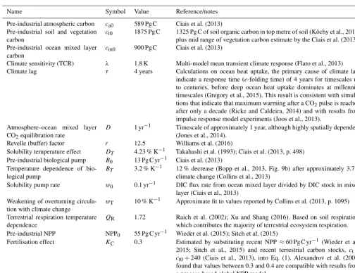
cal-Table 1.Model parameters.
Name Symbol Value Reference/notes
Pre-industrial atmospheric carbon ca0 589 Pg C Ciais et al. (2013)
Pre-industrial soil and vegetation carbon
ct0 1875 Pg C 1325 Pg C of soil organic carbon in top metre of soil (Köchy et al., 2015)
plus mid range of vegetation carbon estimate by the Ciais et al. (2013). Pre-industrial ocean mixed layer
carbon
cm0 900 Pg C Ciais et al. (2013)
Climate sensitivity (TCR) λ 1.8 K Multi-model mean transient climate response (Flato et al., 2013) Climate lag τ 4 years Calculations on ocean heat uptake, the primary cause of climate lag,
indicate a response time (e-folding time) of 4 years for timescales up to centuries, before deep ocean heat uptake dominates at millennial timescales (Gregory et al., 2015). This result is consistent with simula-tions that indicate that maximum warming after a CO2pulse is reached
after only a decade (Ricke and Caldeira, 2014) and with results from impulse response model experiments (Joos et al., 2013).
Atmosphere–ocean mixed layer CO2equilibration rate
D 1 yr−1 Timescale of approximately 1 year, although highly spatially dependent (Jones et al., 2014).
Revelle (buffer) factor r 12.5 Williams et al. (2016)
Solubility temperature effect DT 4.23 % K−1 Takahashi et al. (1993); Ciais et al. (2013, p. 498)
Pre-industrial biological pump B0 13 Pg C yr−1 Ciais et al. (2013)
Temperature dependence of bio-logical pump
BT 3.2 % K−1 12 % decrease (Bopp et al., 2013, Fig. 9b) after approximately 3.7 K
climate change (Collins et al., 2013)
Solubility pump rate w0 0.1 yr−1 DIC flux rate from ocean mixed layer divided by DIC stock in mixed
layer (Ciais et al., 2013) Weakening of overturning
circula-tion with climate change
wT 10 % K−1 Approximate fit to values reported by Collins et al. (2013, p. 1095)
Terrestrial respiration temperature dependence
QR 1.72 Raich et al. (2002); Xu and Shang (2016). Based on soil respiration,
which contributes the majority of terrestrial ecosystem respiration. Pre-industrial NPP NPP0 55 Pg C yr−1 Wieder et al. (2015); Sitch et al. (2015)
Fertilisation effect KC 0.3 Estimated by substituting recent NPP ≈60 Pg C yr−1 (Wieder et al.,
2015; Sitch et al., 2015) and recent terrestrial carbon stocks, ct≈ ct0+240 (Ciais et al., 2013), into Eq. (1). Alexandrov et al. (2003)
found that values between 0.3 and 0.4 are compatible with results from a process-based global NPP model.
culate climate–carbon cycle feedbacks analytically and nu-merically, and estimate feedback non-linearities.
4.1 Definitions
There are multiple measures of carbon cycle feedbacks cur-rently in use. We here review three of the most common mea-sures.
Consider an emission ofEPg C over some time period to the atmosphere. In the absence of carbon cycle feedbacks, the atmospheric carbon content would increase by 1caoff≡E. With a feedback switched on, the atmospheric carbon con-tent would actually change by1cona . The feedback factor is (Zickfeld et al., 2011)
F = 1c
on a
1coff a
. (11)
Out of the total atmospheric carbon change1cona , the carbon cycle feedback contributes (Hansen et al., 1984)
1cafeedback=1caon−1coffa . (12) Gain is the change in a feedback to atmospheric carbon con-tent caused by changes in atmospheric carbon concon-tent:
g=1c
feedback a
1con a
. (13)
Gain and feedback factor are related by
F = 1
1−g. (14)
changes in global mean temperature and atmospheric carbon dioxide as follows:
1ct=βL1ca+γL1T (15)
1cM=βO1ca+γO1T . (16)
Here the βL andβO feedback parameters are the land and
ocean, respectively, carbon sensitivities to atmospheric car-bon dioxide changes1ca. Likewise,γLandγO are the land
and ocean, respectively, carbon sensitivities to temperature changes 1T. Note thatcM denotes the total marine carbon
stock, both mixed layer and deep ocean. The differences1ca,
etc., are usually calculated over the duration of a simulation. To isolate theβandγ feedback parameters, simulations are conducted with biogeochemical coupling only and with ra-diative coupling only (Gregory et al., 2009).
In both the formalisms introduced thus far, the feedback measures are calculated by examining the changes in car-bon stocks at the end point of model simulations. In con-trast, Boer and Arora (2009) estimate sensitivities0andB of the instantaneous carbon fluxes from atmosphere to land and ocean:
dct
dt =BL1ca+0L1T (17)
dcM
dt =BO1ca+0O1T . (18)
These feedback parameters B and0 are usually computed for all time points during a simulation, again using biogeo-chemically coupled and radiatively coupled simulations.
The two sets of parameters (B,0) and (β,γ) are related by
β1ca=
Z
B1cadt (19)
γ 1T = Z
01Tdt. (20)
Accordingly, Boer and Arora (2013) refer toBand0as di-rect feedback parameters and toβ andγ as time-integrated feedback parameters.
4.2 Analytical feedback strengths based on equilibrium changes
Analytical approximations to the strengths of carbon cycle feedbacks in our model require choosing a timescale on which the feedbacks will be calculated. Numerically esti-mated feedback factors (Eq. 11) and time-integrated feed-back parameters (Eqs. 15–16) are conventionally calculated using carbon stock changes over 100 years or more. Re-sponses on the longest timescales of our model are therefore most relevant if our analytical approximations are to approx-imate numerically calculated values. While recognising that the Earth’s climate system is presently far from equilibrium,
we use changes in the equilibrium state of the model to ap-proximate model responses over long timescales.
We analytically calculate the gains associated with each of the feedback loops in Fig. 1 as follows. We calculate the sensitivity (mathematically, partial derivative) of the equilib-rium value of each quantity in the feedback loop with respect to the preceding quantity in the loop. We form the product of the derivatives (as per the chain rule of differentiation) to es-timate the gain of that feedback loop. For example, to calcu-late the land climate–carbon gain we calcucalcu-late the sensitivity of equilibrium temperature with respect to changes in atmo-spheric carbon content (∂T∗/∂ca), multiplied by the
sensitiv-ity of equilibrium terrestrial carbon with respect to changes in temperature (∂ct∗/∂T), multiplied by the sensitivity of equilibrium atmospheric carbon with respect to changes in terrestrial carbon (∂c∗a/∂ct).
Land climate–carbon equilibrium gain.
gTL∗ ≡∂T
∗
∂ca
∂c∗t ∂T
∂ca∗ ∂ct
Land concentration–carbon equilibrium gain.
gL∗≡∂c
∗ t
∂ca
∂c∗a ∂ct
Ocean climate–carbon equilibrium gain.
gTO∗ ≡∂T
∗
∂ca
∂cM
∂T ∂c∗a ∂cM
Ocean concentration–carbon equilibrium gain.
gO∗ ≡∂cM
∂ca
∂c∗a ∂cM
The subscriptT denotes that the feedback involves tempera-ture. Asterisks (∗) denote equilibrium quantities. From these gains, the feedback factorsFTL∗ ,FL∗,FTO∗ , andFO∗can be cal-culated using Eq. (14). We label these gain and feedback fac-torsg∗andF∗, respectively, to denote they are based on an equilibrium approximation, not directly from transient simu-lations as estimated by Zickfeld et al. (2011).
The derivatives ofc∗aare trivial to calculate: by carbon bal-ance,∂c
∗
a
∂ct =
∂c∗
a
∂cM = −1. To calculate the derivatives ofc ∗ T, we
set 0=dct
dt, solve forct, and calculate the necessary
deriva-tives. A similar procedure provides∂T∂c∗
a.
The remaining derivatives are ∂cM
∂T and ∂cM
∂ca. Carbon sunk into the deep ocean is substantial and cannot be neglected. Deep ocean carbon storage equilibrates on timescales of mil-lennia or more, however, far longer than the timescales of interest in this model (we therefore write derivatives ofcM
rather thanc∗M). We therefore cannot use the same equilib-rium approach as for the other variables. Instead, we derive approximations to Eq. (7) as follows. First, we observe that in the SRES A2 scenario used below, bothcm(t) and1T(t)
can be approximated as linear increases, starting atcm=cm0
and1T =0, respectively, over a time intervaltlin. We
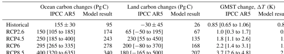
us-Table 2.Model validation. Historical changes are carbon stocks in 2011 relative to stocks in 1750 (Ciais et al., 2013) and temperatures in 2012 relative to temperatures in 1880 (Hartmann et al., 2013). Predicted future changes are carbon stocks in 2100 compared to 2012 (Collins et al., 2013) and global mean surface temperature (GMST) averaged over 2081–2100 relative to 1986–2005 (Collins et al., 2013), under the range of RCP scenarios.
Ocean carbon changes (Pg C) Land carbon changes (Pg C) GMST change,1T (K) IPCC AR5 Model result IPCC AR5 Model result IPCC AR5 Model result
Historical 155±30 95 −30±45 26 0.85 [0.65 to 1.06] 0.82
RCP2.6 150 [105 to 185] 174 65 [−50 to 195] 67 1.0 [0.3 to 1.7] 0.5
RCP4.5 250 [185 to 400] 243 230 [55 to 450] 135 1.8 [1.1 to 2.6] 1.2
RCP6 295 [265 to 335] 278 200 [−80 to 370] 168 2.2 [1.4 to 3.1] 1.7
RCP8.5 400 [320 to 635] 340 180 [−165 to 500] 207 3.7 [2.6 to 4.8] 2.4
ing the valuecmand gradientc0mat the end of the simulation
period. We obtain
1cM≈cm−cm0+w0
1
2− 1 3wT1T
cm−cm0
tlin
−1
2B0BT1T tlin. (21)
We use this equation to calculate the derivatives ∂cM
∂T and ∂cM
∂ca. Evaluating these derivatives will involve the deriva-tives ∂cm
∂T and ∂cm
∂ca. Since partial pressures across the air–sea interface equilibrate rapidly on the timescale of the model (D=1 yr−1, Table 1), we assume thatc
a≈p(cm, 1T),
re-arrange forcm, and then calculate the appropriate derivatives
from the resulting equation.
We analytically estimate equilibrium versions of the time-integrated feedback parameters of Friedlingstein et al. (2006) using a similar approach:
γL∗=∂c
∗ t
∂T
βL∗=∂c
∗ t
∂ca
γO∗=∂cM
∂T
βO∗=∂cM
∂ca
.
Since the ocean component of the model has multiple pro-cesses that respond to temperature, some analytical forms were too complicated for easy visual inspection (Table A1). We derived approximate analytical feedbacks by comparing the magnitudes of terms in the numerator and denominator of the feedback measures by expanding in power series ofDTT
andca/ca0.
4.3 Analytical feedback strengths based on carbon fluxes
We estimate the direct feedback parameters as follows:
0L∗= dct
dt
ca=ca0 1 1T
BL∗= dct
dt
1T=0
1 ca−ca0
0∗O= dcM
dt c
a=ca0
1 1T
BO∗= dcM
dt
1T=0
1 ca−ca0
.
Here dct/dt and dcM/dt denote the atmosphere–land and
atmosphere–ocean fluxes. The subscript 1T =0 denotes a biogeochemically coupled (and radiatively decoupled) sim-ulation andca=ca0denotes a radiatively coupled (and
bio-geochemically decoupled) simulation.
The values of the feedback parameters are strongly sce-nario dependent (Arora et al., 2013). To calculate the di-rect feedback parameters, we assume a standard CO2
-quadrupling concentration pathway in order to compare our results with Arora et al. (2013). This scenario hasca(t)=
ca0at, where a=1.01. In this scenario, c1
a
dca
dt =loga and,
ignoring an initial exponential transient,dTdt =λloga/log 2. For the atmosphere–land carbon flux, the calculation is straightforward under the following assumptions. We as-sume that NPP0/ct0loga so that ct tracks its carrying
capacity ct≈K (Eq. 2). We also ignore land use change,
so that dct
dt ≈ dK
dt. Then we calculate dK
dt |ca=ca0=
∂K ∂T
dT dt and dK
dt |1T=0= ∂K ∂ca
dca
dt .
While the atmosphere–ocean flux could be read off di-rectly from the first term of Eq. (6), this form is however not particularly useful. As it involves a small difference be-tween two large quantities,caandp(cm, 1T), the size of the
difference can only be estimated from numerical results and gives no immediate insight into how it depends on parame-ters. Furthermore, we seek to compare our analytical results to the results presented by Arora et al. (2013), in which the feedback parameters are presented as functions ofcaor1T
only (notcm).
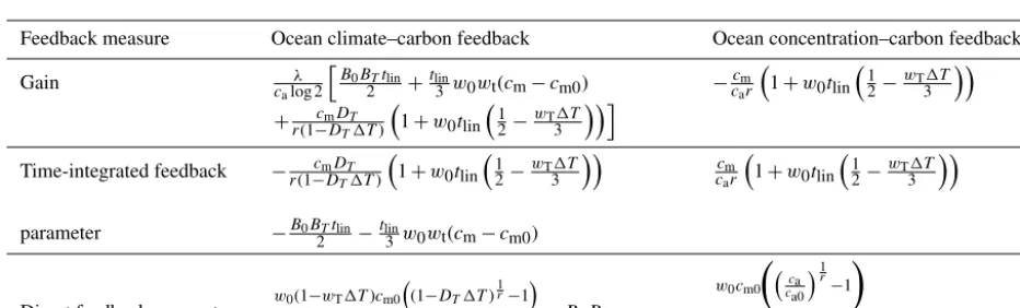
Table 3.Feedback analysis. Gains (g), feedback factors (F), time-integrated feedback parameters (γandβ), and direct feedback parameters (0andB) were calculated analytically and numerically. Analytical ocean feedbacks are approximations of the exact forms in Table A1 (see Sect. 4.2). Exact forms were used to calculate numerical values. In this table, p≡p(cm, T). Units of the climate–carbon integrated
feedback parameters are Pg C K−1and concentration–carbon integrated feedback parameters are Pg C ppm−1. Ranges for analytical results are written in the form (value at start of simulation) to (value at end of simulation). Emissions scenarios are as indicated; land use emissions were assumed to be zero. From the results of simulations using the SRES A2 scenario we usetlin≈100 corresponding to a period between
the years 2000 and 2100.
Feedback measure Land climate– Ocean climate– Land conc.– Ocean conc.–
carbon feedback carbon feedback carbon feedback carbon feedback
Gain, analytical expression
λct0
1+KClogcca0a
logQR
10caQ1T /10R log 2
λtlin calog 2
B0BT
2 +
cmDTw0
2r
+w0wT(cm−cm0) 3
− ct0KC caQ1T /10R
−cmw0tlin 2car
Feedback factor (numerical scenario: SRES A2) (>1 amplifies climate change;<1 dampens climate change)
– estimate from analytical gain 1.81 to 1.18 1.01 to 1.09 0.51 to 0.81 0.89 to 0.84
– from simulation 1.15 1.10 0.80 0.73
– Zickfeld et al. (2011) 1.25 1.22 0.66 0.71
Time-integrated feedback parameter (numerical scenario: SRES A2) (<0 amplifies climate change;>0 dampens climate change)
– analytical expression −ct0logQR 10Q1T /10R
−B0BT tlin
2 −
cmDTw0tlin
2r ct0KC ca
cmw0tlin
2car
−w0wt(cm−cm0) tlin
3
– estimate from analytical form −102 to−86 −3 to−67 2.04 to 0.51 0.26 to 0.42
– from simulation −74 −48 0.84 1.09
– Zickfeld et al. (2011) −129 −32 1.32 0.98
– Friedlingstein et al. (2006) −79 (−20 to−177) −30 (−14 to−67) 1.35 (0.2 to 2.8) 1.13 (0.8 to 1.6) Direct feedback parameter (numerical scenario: CO2doubling) (<0 amplifies climate change;>0 dampens climate change)
– analytical expression −ct0λlogQRloga
101Tlog 2 −
w0cm0DT r −B0BT
ct0KCloga ca−ca0
w0cm rca
– estimate from analytical form Fig. A1a Fig. A1b Fig. A1a Fig. A1b
– from simulation Fig. A1a Fig. A1b Fig. A1a Fig. A1b
– Arora et al. (2013) see text
Non-linearity −0.43 −0.11 0.03 0.03
diffusion is the fastest process, ocean mixed layer carbon content rapidly gains an equilibriumcm=p−1(ca, 1T) with
respect to atmospheric carbon content, where p−1(ca, 1T)
is the solution to ca=p(cm, 1T). On the timescale of our
model, the atmosphere–ocean flux is therefore controlled by the solubility and biological pumps, with diffusion provid-ing a rapid couplprovid-ing between ocean mixed layer and atmo-sphere. An approximation for the atmosphere–ocean flux is therefore dcMdt−1≈w0(1−wT1T)(p−1(ca, 1T)−cm0)−
B0BTT, which upon substitution into the definitions ofBO∗
and0∗Ogives the forms in Table A1. Taylor series expansions and L’Hôpital’s rule were then used to derive the approximate forms in Table 3.
4.4 Numerical estimation of feedback strengths
In addition to the analytical approximations to carbon cycle feedbacks derived from our model, we also estimate
feed-back factors from direct numerical simulations of our model. To compare the results of our model to previous studies, we use the following scenarios. To compare our results with the time-integrated feedback parameters reported by Friedling-stein et al. (2006) and the feedback factors and gains of Zickfeld et al. (2011), we employ the SRES A2 emissions scenario used in those articles. To compare our results with the direct feedback parameters of Arora et al. (2013), we use the same scenario used in that article in which CO2
concen-tration increases 1 % yr−1until it quadruples (approximately 140 years). For each scenario, we perform four simulations:
1. Fully coupled simulation.
2. Completely uncoupled simulation, giving coffa (t)=
ca0+
Rt
3. Biogeochemically coupled simulation. We switch off feedbacks involving temperature response to atmo-spheric CO2by settingλ=0. Since our model contains
no radiative forcing other than changes in CO2,
temperature1T =0 in this simulation. From this sim-ulation we estimate the carbon–concentration feedback factors via land FL=1cona /1caoff=1−1ct/1coffa
and ocean FO=1cona /1caoff=1−1cM/1coffa ,
time-integrated feedback parameters βL=1ct/1ca and
βO=1cM/1ca, and direct feedback parameters
BL(t)=dcdtt/(ca−ca0) andBO(t)=dcdtM/(ca−ca0).
4. Radiatively coupled simulation. We switch off feed-backs involving the carbon cycle, by setting KC=0
and changing the ca in Eq. (6) toca0. From this
sim-ulation we estimate the carbon–climate feedback fac-tors FTL=1−1ct/1coffa andFTO=1−1cM/1coffa ,
time-integrated feedback parametersγL=1ct/1T and
γO=1cM/1T following Arora et al. (2013), and
di-rect feedback parameters0L(t)=dcdtt/1T and0O(t)= dcM
dt /1T.
4.5 Feedback non-linearity
Zickfeld et al. (2011) found, in emissions-driven scenarios, that the fully coupled simulation sunk more terrestrial and marine carbon than the sum of the biogeochemically and radiatively coupled scenarios. They refer to this difference as the non-linearity of the feedback, with the land sink con-tributing 80 % of the non-linearity and the ocean sink 20 %. Our analytical expressions for the feedbacks can be used to obtain an alternative measure of feedback non-linearity.
We evaluate the non-linearity in the ocean and land climate–carbon feedbacks using FTO∗ (ca, cm, ct, 1T)−
FTO∗ (ca0, cm0, ct0, 1T) and FTL∗ (ca, cm, ct, 1T)−
FTL∗ (ca0, cm0, ct0, 1T), respectively, where the
F∗(ca0, cm0, ct0, 1T) are analytical approximations of
feedback factors from a radiatively coupled simulation (all carbon stocks are fixed at pre-industrial levels). We evaluate the non-linearities in the ocean and land concentration– carbon feedbacks usingFO∗(ca, cm, ct, 1T)−FO∗(ca, cm, ct,0)
andFL∗(ca, cm, ct, 1T)−FL∗(ca, cm, ct,0), respectively, where
the F∗(ca, cm, ct,0) are analytical approximations of
feed-back factors from a biogeochemically coupled simulation (temperature is fixed at its pre-industrial level). These ex-pressions indicate the effect of temperature and atmospheric carbon on the concentration–carbon and climate–carbon feedbacks, respectively, We used the SRES A2 scenario.
5 Results and discussion
5.1 Model evaluation
Most predictions of our model are within the range of model predictions produced for the IPCC’s Fifth Assessment
Re-port (Table 2). Our model estimates around 55 Pg C more historical land carbon uptake than the IPCC multi-model mean, possibly due to our simplification to a single land car-bon pool. Because it omits radiative forcing due to green-house gases other than CO2, our model consistently
underes-timates future temperature changes, although in all except the RCP8.5 scenario the projections are within the IPCC model range. The purpose of our model is not to precisely predict future climate change, but to serve as an approximate, mech-anistically based emulator of the carbon cycle component of Earth system models (see Sect. 2). If we choose param-eters to fit historical observations rather than based on the best available knowledge about each process (see Sect. 3), then our results remain mostly within IPCC model range al-though ocean and land uptake are consistently above and be-low the IPCC multi-model mean, respectively (Table A2a). We conclude that the model emulates historical observations and future projections of Earth system models with sufficient accuracy for this purpose.
5.2 Feedback analysis
All feedback measures calculated directly from our stylised model simulations, as well as most of our analytically es-timated feedback measures, are within a factor of 2 of the mean output from Earth system models reported by Friedlingstein et al. (2006) and Zickfeld et al. (2011) (Ta-ble 3; compare also Fig. A1 with Figs. 4–5 of Arora et al. (2013) for direct feedback parameters). This is a remarkably good agreement considering the highly stylised nature of our model. Furthermore, all of the numerically time-integrated feedback parameters from our stylised model are within the multi-model range reported by Friedlingstein et al. (2006). The agreement observed here serves as additional validation of our model as well as validation of the approximations used to calculate analytical feedback factors.
An exception to the close agreement is the ocean concentration–carbon feedback, with the analytically esti-mated feedback factor and time-integrated feedback parame-ter indicating a weaker negative feedback than the numerical estimates from our stylised model or Earth system models. This mismatch is primarily due to two approximations: one in the numerical simulation and one in the analytical approx-imation. The numerical approximation is that disconnecting climate feedbacks in the biogeochemically coupled simula-tion leaves less carbon available to be sunk into the ocean, placing the ocean feedback at a different point in the highly non-linear (as parameterised by the Revelle factor) ocean car-bon uptake dynamics. The analytical approximation is that Eq. (21) underestimates carbon sunk into the deep ocean.
be-came more positive and the already negative concentration– carbon feedbacks more negative. The numerical feedback es-timates retained, however, good agreement with analytical estimates as well as with previous numerical estimates by Friedlingstein et al. (2006) and Zickfeld et al. (2011). One exception was the ocean concentration–carbon feedback, for which the analytical estimate remained outside Friedling-stein et al.’s range as noted above, but the direct numerical estimate moved to also be outside their range. We conclude that our results are relatively insensitive to parameter val-ues, though mechanistically based parameter values perform slightly better than fitted parameter values.
Focusing on the analytical expressions, we observe that the approximate analytical expressions for the three dif-ferent feedback measures all have similar dependences on state variables and parameters. All measures of the land climate–carbon feedback have dependence of the form ct0logQR/Q1T /10R . The ocean climate–carbon feedbacks all
have terms of the form B0BT and w0DTcm/r. The land
concentration–carbon feedback has the form ct0KC/ca and
the ocean concentration–carbon feedbacks have the form w0cm/rca. We conclude that for each type of carbon cycle
feedback, all three feedback formalisms detect similar fea-tures of the climate–carbon system.
The analytical expressions provide rapid insight into how feedback strengths depend on state variable and parameter values that could otherwise only be studied numerically or by qualitative reasoning. The analytical forms show that in-creasing Revelle factorr, as is likely to occur in an increas-ingly acidic ocean (Sabine et al., 2004), will decrease the strengths of ocean climate–carbon and concentration–carbon feedbacks. Weakening overturning circulation, viaw0, would
also decrease the strength of the ocean carbon cycle feed-backs. On land, the parametersQRandKCcontrol the
ter-restrial carbon cycle feedbacks.
We can compare likely trends in feedback strengths from the analytical expressions for the direct feedback pa-rameters. According to our model, the destabilising ocean climate–carbon feedback is almost constant, while the ocean concentration–carbon feedback weakens with cm (since
cm/ca∼c1m−r). Similarly, according to our model the
desta-bilising land climate–carbon feedback will weaken less than the stabilising concentration–carbon feedback (under CO2
doubling, ∼Q−R1T /10 weakens by 9 % at the new temper-ature equilibrium while∼1/caweakens by 50 %). This
dif-ference between the land climate–carbon and concentration– carbon feedbacks stems from the differing curvatures of K(ca, 1T) as a function of1T (close to linear) andca
(con-cave). We conclude that under continued carbon emissions, according to our model, both land and ocean feedbacks will overall become more positive.
Where multiple processes contribute in parallel to a feed-back, inspection of analytical forms can indicate the relative contributions of the different processes to the feedback. In
the ocean component of the model, CO2solubility, the
bio-logical pump, and the solubility pump are all temperature de-pendent and therefore contribute to the ocean climate–carbon feedback. Remarkably, all three processes contribute tem-perature dependences of a similar magnitude; we therefore list all three in the approximate analytical gain and time-integrated feedback parameter in Table 3. The three terms represent temperature dependence of the biological pump, CO2solubility, and the solubility pump.
5.3 Feedback non-linearity
As shown in Sect. 4.5, our analytical feedback expressions enable a new way of estimating feedback non-linearities that is not possible from direct numerical simulation. Since the sum of the four non-linearities is negative (Table 3), we con-clude that summing feedbacks found by individual decou-pled simulations will overestimate the atmospheric carbon levels, that is, underestimate land and ocean sinks. This result matches the findings of Zickfeld et al. (2011) and Matthews (2007). Terrestrial feedbacks contributed 83 % of the to-tal non-linearity in our model, compared to 80 % reported by Zickfeld et al. (2011). Furthermore, we can distinguish the non-linearities in the climate–carbon and concentration– carbon feedbacks. We found that the non-linearity in the ter-restrial carbon–climate feedback was almost 4 times larger than any other (Table 3). By inspecting the analytical deriva-tion of the gains we conclude that this dominance is likely due to a combination of three reasons: first, due to the sensi-tivity of temperature to carbon dioxide,∂T /∂ca=λ/calog 2,
the carbon–climate feedbacks are much more sensitive toca
than the concentration–carbon feedbacks are to 1T. Sec-ond, the non-linearity in the land climate–carbon feedback is larger than the ocean climate–carbon feedback because its feedback factor is larger and therefore more sensitive to changes in gain (see Eq. 13). Third, the century timescale of the simulation prevented ocean carbon dynamics, which generally take place on longer timescales, from being exhib-ited. We conclude that care must be taken when summing results for feedbacks from decoupled simulations, especially for simulations involving land feedbacks.
6 Conclusions
carbon cycle model could be a starting point for model-based investigations of Earth system processes that are too poorly understood to be incorporated in more comprehensive mod-els.
Stylised models such as ours have significant value in pol-icy contexts. When confronted with difficult polpol-icy decisions involving long time periods and significant uncertainty, col-laborative work with scientists allows policymakers to iden-tify and clarify the impacts of various policy actions. In this context, the utility of a model is to increase stakeholders’ un-derstanding of a system and its dynamics under various con-ditions (Voinov and Bousquet, 2010; Anderies, 2005). This is in stark contrast to the use of more comprehensive models to predict impacts of policies in which mechanisms under-lying dynamics and trade-offs are not transparent and quick explorations with stakeholders are not practical. The utility of a stylised model is in facilitating a learning process rather than in “accurately” predicting outcomes.
We foresee at least two strands of valuable future research based on the climate–carbon cycle model developed in this paper. First, our climate–carbon cycle model could be ex-tended by including further processes relevant on different timescales of interest for Earth system analysis. This would enable a more in-depth analytical analysis of the feedback strengths and gains relating to other aspects of Earth system dynamics, such as the Earth’s energy balance, carbon storage in the tropics compared to extratropics, albedo changes, the cryosphere, nutrient cycles, and even societal feedbacks. The task of characterising the Anthropocene as an epoch could thus move beyond qualitative comparison of human-impact trends to an improved characterisation of the feedbacks that maintain different Earth system “regimes”. The effects on feedback strengths of different functional forms, such as the fertilisation effectKC, and how to constrain these functional
forms from data could also be investigated and could yield insight into the continued divergence of Earth system model projections.
Second, the model could comprise a workbench for the systemic understanding of planetary boundary interactions and hence generate crucial insights into the structure of the safe operating space for humanity delineated by the plane-tary boundaries (Rockström et al., 2009; Steffen et al., 2015). Such extensions should focus on linking the core abiotic and biotic dimensions of the planetary boundary framework. The present lack of well-developed model representations of the dynamics and ecosystem structure of biosphere di-versity, heterogeneity, and resilience, despite ongoing efforts in this direction (Purves et al., 2013; Bartlett et al., 2016; Sakschewski et al., 2016), emphasises the need for a more conceptual understanding of biosphere integrity, its vulner-ability to anthropogenic perturbation, and its role for Earth system resilience.
Appendix A
(a) (b)
400 600 800 1000
0.01 0.02 0.03 0.04 0.05 0.06
Atmospheric CO2, ca(ppm)
B
(P
gC
/p
pm
y
r
-1)
BL(numerical) BO(numerical)
BL(analytical) BO(analytical) - 10
- 8 - 6 - 4 - 2
00 1 2 3 4
Γ
(P
gC
/K
y
r
-1)
Temperature, ΔT (K)
ΓL(numerical) ΓO(numerical)
ΓL(analytical) ΓO(analytical)
Figure A1.Direct feedback parameters,(a)climate–carbon feedbacks, and(b)concentration– carbon feedbacks.
Table A1.Exact forms for ocean feedbacks.
Feedback measure Ocean climate–carbon feedback Ocean concentration–carbon feedback
Gain c λ
alog 2
h B0BTtlin
2 + tlin
3 w0wt(cm−cm0)
+ cmDT
r(1−DT1T)
1+w0tlin
1 2−
wT1T
3 i
−cm
car
1+w0tlin
1 2−
wT1T
3
Time-integrated feedback − cmDT
r(1−DT1T)
1+w0tlin
1 2−
wT1T
3
c
m
car
1+w0tlin
1 2−
wT1T
3
parameter −B0BTtlin
2 − tlin
3w0wt(cm−cm0)
Direct feedback parameter w0(1
−wT1T)cm0
(1−DT1T) 1 r−1
1T −B0BT
w0cm0
ca ca0
1r −1
!
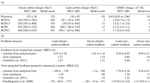
Table A2.Testing parameters fitted to historical data. The following changes to parameter values were made to those listed in Table 1:KC=
0.25,QR=2.45,λ=1.91 K,w0=0.185 yr−1.(a)Historical and projected changes of carbon stocks. See Table 2 for further information
on how the figures were calculated and sources for model comparison.(b)Feedback analysis. See Table 3 for further information. Analytical forms are omitted here.
(a)
Ocean carbon changes (Pg C) Land carbon changes (Pg C) GMST change,1T (K)
IPCC AR5 Model result IPCC AR5 Model result IPCC AR5 Model result
Historical 155±30 155 −30±45 −30 0.85 [0.65 to 1.06] 0.85
RCP2.6 150 [105 to 185] 303 65 [−50 to 195] 2 1.0 [0.3 to 1.7] 0.3
RCP4.5 250 [185 to 400] 428 230 [55 to 450] 11 1.8 [1.1 to 2.6] 1.2
RCP6 295 [265 to 335] 484 200 [−80 to 370] 13 2.2 [1.4 to 3.1] 1.7
RCP8.5 400 [320 to 635] 591 180 [−165 to 500] −7 3.7 [2.6 to 4.8] 2.5
(b)
Feedback measure Land climate– Ocean climate– Land conc.– Ocean conc.–
carbon feedback carbon feedback carbon feedback carbon feedback
Feedback factor (numerical scenario: SRES A2)
– estimate from analytical gain 4.67 to 1.30 1.01 to 1.16 0.56 to 0.85 0.89 to 0.75
– from simulation 1.27 1.14 0.84 0.60
– Zickfeld et al. (2011) 1.25 1.22 0.66 0.71
Time-integrated feedback parameter (numerical scenario: SRES A2)
– estimate from analytical form −168 to−126 −3 to−100 1.70 to 0.38 0.26 to 0.70
– from simulation −119 −60 1.28 1.92
– Zickfeld et al. (2011) −129 −32 1.32 0.98
– Friedlingstein et al. (2006) −79 (−20 to−177) −30 (−14 to−67) 1.35 (0.2 to 2.8) 1.13 (0.8 to 1.6)
Author contributions. SJL, JMA, SEC, JFD, IF, KR, JR, and WS designed the research. SJL, JFD, IF, TG, and CB constructed the model. SJL analysed the model. All authors wrote the paper.
Competing interests. The authors declare that they have no con-flict of interest.
Special issue statement. This article is part of the special issue “Social dynamics and planetary boundaries in Earth system mod-elling”. It is not associated with a conference.
Acknowledgements. The research leading to these results has received funding from the Stordalen Foundation via the Planetary Boundary Research Network (PB.net), the Earth League’s Earth-Doc programme, the Leibniz Association (project DOMINOES), European Research Council Synergy project Imbalance-P (grant ERC-2013-SyG-610028), project grant 2014-589 from the Swedish Research Council Formas, and a core grant to the Stockholm Resilience Centre by Mistra. We thank Malin Ödalen for her comments on the paper.
Edited by: Axel Kleidon
Reviewed by: Martin Heimann and Chris Jones
References
Alexandrov, G., Oikawa, T., and Yamagata, Y.: Climate dependence of the CO2fertilization effect on terrestrial net primary
produc-tion, Tellus B, 55, 669–675, 2003.
Anderies, J. M.: Minimal models and agroecological policy at the regional scale: an application to salinity problems in southeastern Australia, Reg. Environ. Change, 5, 1–17, 2005.
Anderies, J. M., Carpenter, S. R., Steffen, W., and Rockström, J.: The topology of non-linear global carbon dynamics: from tipping points to planetary boundaries, Environ. Res. Lett., 8, 044048, https://doi.org/10.1088/1748-9326/8/4/044048, 2013.
Arora, V. K., Boer, G. J., Friedlingstein, P., Eby, M., Jones, C. D., Christian, J. R., Bonan, G., Bopp, L., Brovkin, V., Cadule, P., Bala, G., John, J., Jones, C., Joos, F., Kato, T., Kawamiya, M., Knorr, W., Lindsay, K., Matthews, H. D., Raddatz, T., Rayner, P., Reick, C., Roeckner, E., Schnitzler, K.-G., Schnur, R., Strass-mann, K., Weaver, A. J., Yoshikawa, C., and Zeng, N.: Carbon– concentration and carbon–climate feedbacks in CMIP5 Earth system models, J. Climate, 26, 5289–5314, 2013.
Bacastow, R., Keeling, C. D., Woodwell, G., and Pecan, E.: Atmo-spheric carbon dioxide and radiocarbon in the natural carbon cy-cle, II. Changes from AD 1700 to 2070 as deduced from a geo-chemical model, Tech. rep., Univ. of California, San Diego, La Jolla; Brookhaven National Lab., Upton, NY, USA, 1973. Bartlett, L. J., Newbold, T., Purves, D. W., Tittensor, D. P., and
Harfoot, M. B.: Synergistic impacts of habitat loss and frag-mentation on model ecosystems, P. Roy. Soc. B, 283, 20161027, https://doi.org/10.1098/rspb.2016.1027, 2016.
Bernardello, R., Marinov, I., Palter, J. B., Sarmiento, J. L., Gal-braith, E. D., and Slater, R. D.: Response of the ocean natural
carbon storage to projected twenty-first-century climate change, J. Climate, 27, 2033–2053, 2014.
Boer, G. and Arora, V.: Temperature and concentration feed-backs in the carbon cycle, Geophys. Res. Lett., 36, L02704, https://doi.org/10.1029/2008GL036220, 2009.
Boer, G. and Arora, V.: Feedbacks in emission-driven and concentration-driven global carbon budgets, J. Climate, 26, 3326–3341, 2013.
Bopp, L., Resplandy, L., Orr, J. C., Doney, S. C., Dunne, J. P., Gehlen, M., Halloran, P., Heinze, C., Ilyina, T., Séférian, R., Tjiputra, J., and Vichi, M.: Multiple stressors of ocean ecosys-tems in the 21st century: projections with CMIP5 models, Biogeosciences, 10, 6225–6245, https://doi.org/10.5194/bg-10-6225-2013, 2013.
Ciais, P., Sabine, C., Bala, G., Bopp, L., Brovkin, V., Canadell, J., Chhabra, A., DeFries, R., Galloway, J., Heimann, M., Jones, C., LeQuéré, C., Myneni, R., Piao, S., and Thornton, P.: Carbon and Other Biogeochemical Cycles, book section 6, Cambridge Uni-versity Press, Cambridge, UK and New York, NY, USA, 465– 570, https://doi.org/10.1017/CBO9781107415324.015, 2013. Collins, M., Knutti, R., Arblaster, J., Dufresne, J.-L., Fichefet, T.,
Friedlingstein, P., Gao, X., Gutowski, W., Johns, T., Krin-ner, G., Shongwe, M., Tebaldi, C., Weaver, A., and WehKrin-ner, M.: Long-term Climate Change: Projections, Commitments and Ir-reversibility, book section 12, Cambridge University Press, Cambridge, UK and New York, NY, USA, 1029–1136, https://doi.org/10.1017/CBO9781107415324.024, 2013. Flato, G., Marotzke, J., Abiodun, B., Braconnot, P., Chou, S.,
Collins, W., Cox, P., Driouech, F., Emori, S., Eyring, V., Forest, C., Gleckler, P., Guilyardi, E., Jakob, C., Kattsov, V., Reason, C., and Rummukainen, M.: Evaluation of Cli-mate Models, book section 9, Cambridge University Press, Cambridge, UK and New York, NY, USA, 741–866, https://doi.org/10.1017/CBO9781107415324.020, 2013. Friedlingstein, P.: Carbon cycle feedbacks and future
cli-mate change, Philos. T. Roy. Soc. A, 373, 20140421, https://doi.org/10.1098/rsta.2014.0421, 2015.
Friedlingstein, P., Cox, P., Betts, R., Bopp, L., Von Bloh, W., Brovkin, V., Cadule, P., Doney, S., Eby, M., Fung, I., Bala, G., John, J., Jones, C., Joos, F., Kato, T., Kawamiya, M., Knorr, W., Lindsay, K., Matthews, H. D., Raddatz, T., Rayner, P., Reick, C., Roeckner, E., Schnitzler, K.-G., Schnur, R., Strassmann, K., Weaver, A. J., Yoshikawa, C., and Zeng, N.: Climate–carbon cy-cle feedback analysis: results from the C4MIP model intercom-parison, J. Climate, 19, 3337–3353, 2006.
Gasser, T., Ciais, P., Boucher, O., Quilcaille, Y., Tortora, M., Bopp, L., and Hauglustaine, D.: The compact Earth system model OS-CAR_v2.2: description and first results, Geosci. Model Dev., 10, 271–319, https://doi.org/10.5194/gmd-10-271-2017, 2017a. Gasser, T., Peters, G. P., Fuglestvedt, J. S., Collins, W. J.,
Shin-dell, D. T., and Ciais, P.: Accounting for the climate–carbon feedback in emission metrics, Earth Syst. Dynam., 8, 235–253, https://doi.org/10.5194/esd-8-235-2017, 2017b.
Goodwin, P., Williams, R. G., Follows, M. J., and Dutkiewicz, S.: Ocean-atmosphere partitioning of anthropogenic carbon dioxide on centennial timescales, Global Biogeochem. Cy., 21, GB1014, https://doi.org/10.1029/2006GB002810, 2007.
Gregory, J. M., Andrews, T., and Good, P.: The incon-stancy of the transient climate response parameter under increasing CO2, Philos. T. Roy. Soc. A, 373, 20140417 https://doi.org/10.1098/rsta.2014.0417, 2015.
Hansen, J., Lacis, A., Rind, D., Russell, G., Stone, P., Fung, I., Ruedy, R., and Lerner, J.: Climate sensitivity: analysis of feed-back mechanisms, in: Climate Processes and Climate Sensitivity, AGU Geophysical Monograph 29, Maurice Ewing Vol. 5, edited by: Hansen, J. E. and Takahashi, T., Washington, D.C., 130–163, 1984.
Harman, I. N., Trudinger, C. M., and Raupach, M. R.: SCCM– the Simple Carbon-Climate Model: Technical Documentation, CAWCR Technical Report No. 047, The Centre for Australian Weather and Climate Research, Canberra, 2011.
Hartmann, D., Klein Tank, A., Rusticucci, M., Alexan-der, L., Brönnimann, S., Charabi, Y., Dentener, F., Dlugo-kencky, E., Easterling, D., Kaplan, A., Soden, B., Thorne, P., Wild, M., and Zhai, P.: Observations: Atmosphere and Surface, book section 2, Cambridge University Press, Cambridge, UK and New York, NY, USA, p. 159–254, https://doi.org/10.1017/CBO9781107415324.008, 2013. Jones, D. C., Ito, T., Takano, Y., and Hsu, W.-C.: Spatial and
sea-sonal variability of the air-sea equilibration timescale of carbon dioxide, Global Biogeochem. Cy., 28, 1163–1178, 2014. Joos, F., Bruno, M., Fink, R., Siegenthaler, U., Stocker, T. F.,
Le Quere, C., and Sarmiento, J. L.: An efficient and accurate representation of complex oceanic and biospheric models of an-thropogenic carbon uptake, Tellus B, 48, 397–417, 1996. Joos, F., Roth, R., Fuglestvedt, J. S., Peters, G. P., Enting, I. G.,
von Bloh, W., Brovkin, V., Burke, E. J., Eby, M., Edwards, N. R., Friedrich, T., Frölicher, T. L., Halloran, P. R., Holden, P. B., Jones, C., Kleinen, T., Mackenzie, F. T., Matsumoto, K., Meinshausen, M., Plattner, G.-K., Reisinger, A., Segschneider, J., Shaffer, G., Steinacher, M., Strassmann, K., Tanaka, K., Tmermann, A., and Weaver, A. J.: Carbon dioxide and climate im-pulse response functions for the computation of greenhouse gas metrics: a multi-model analysis, Atmos. Chem. Phys., 13, 2793– 2825, https://doi.org/10.5194/acp-13-2793-2013, 2013. Kamiuto, K.: A simple global carbon-cycle model, Energy, 19, 825–
829, 1994.
Kellie-Smith, O. and Cox, P. M.: Emergent dynamics of the climate–economy system in the Anthropocene, Philos. T. Roy. Soc. A, 369, 868–886, 2011.
Köchy, M., Hiederer, R., and Freibauer, A.: Global distribution of soil organic carbon – Part 1: Masses and frequency distributions of SOC stocks for the tropics, permafrost regions, wetlands, and the world, SOIL, 1, 351–365, https://doi.org/10.5194/soil-1-351-2015, 2015.
Körner, C.: Carbon limitation in trees, J. Ecol., 91, 4–17, 2003. Kriegler, E., Hall, J. W., Held, H., Dawson, R., and
Schellnhu-ber, H. J.: Imprecise probability assessment of tipping points in the climate system, P. Natl. Acad. Sci. USA, 106, 5041–5046, 2009.
Lenton, T. M.: Land and ocean carbon cycle feedback effects on global warming in a simple Earth system model, Tellus B, 52, 1159–1188, 2000.
Lenton, T. M., Held, H., Kriegler, E., Hall, J. W., Lucht, W., Rahm-storf, S., and Schellnhuber, H. J.: Tipping elements in the Earth’s climate system, P. Natl. Acad. Sci. USA, 105, 1786–1793, 2008.
Le Quéré, C., Andrew, R. M., Canadell, J. G., Sitch, S., Kors-bakken, J. I., Peters, G. P., Manning, A. C., Boden, T. A., Tans, P. P., Houghton, R. A., Keeling, R. F., Alin, S., Andrews, O. D., Anthoni, P., Barbero, L., Bopp, L., Chevallier, F., Chini, L. P., Ciais, P., Currie, K., Delire, C., Doney, S. C., Friedlingstein, P., Gkritzalis, T., Harris, I., Hauck, J., Haverd, V., Hoppema, M., Klein Goldewijk, K., Jain, A. K., Kato, E., Körtzinger, A., Land-schützer, P., Lefèvre, N., Lenton, A., Lienert, S., Lombardozzi, D., Melton, J. R., Metzl, N., Millero, F., Monteiro, P. M. S., Munro, D. R., Nabel, J. E. M. S., Nakaoka, S.-I., O’Brien, K., Olsen, A., Omar, A. M., Ono, T., Pierrot, D., Poulter, B., Röden-beck, C., Salisbury, J., Schuster, U., Schwinger, J., Séférian, R., Skjelvan, I., Stocker, B. D., Sutton, A. J., Takahashi, T., Tian, H., Tilbrook, B., van der Laan-Luijkx, I. T., van der Werf, G. R., Viovy, N., Walker, A. P., Wiltshire, A. J., and Zaehle, S.: Global Carbon Budget 2016, Earth Syst. Sci. Data, 8, 605–649, https://doi.org/10.5194/essd-8-605-2016, 2016.
Matthews, H. D.: Implications of CO2fertilization for future
cli-mate change in a coupled clicli-mate–carbon model, Global Change Biol., 13, 1068–1078, 2007.
Meinshausen, M., Raper, S. C. B., and Wigley, T. M. L.: Em-ulating coupled atmosphere-ocean and carbon cycle models with a simpler model, MAGICC6 – Part 1: Model descrip-tion and calibradescrip-tion, Atmos. Chem. Phys., 11, 1417–1456, https://doi.org/10.5194/acp-11-1417-2011, 2011a.
Meinshausen, M., Smith, S. J., Calvin, K., Daniel, J. S., Kainuma, M., Lamarque, J., Matsumoto, K., Montzka, S., Raper, S., Riahi, K., Thomson, A., Velders, G. J. M., and van Vu-uren, D. P. P.: The RCP greenhouse gas concentrations and their extensions from 1765 to 2300, Climatic Change, 109, 213–241, 2011b.
Meinshausen, M., Wigley, T. M. L., and Raper, S. C. B.: Em-ulating atmosphere-ocean and carbon cycle models with a simpler model, MAGICC6 – Part 2: Applications, Atmos. Chem. Phys., 11, 1457–1471, https://doi.org/10.5194/acp-11-1457-2011, 2011c.
NOAA: Climate at a Glance: Global Time Series, Tech. rep., NOAA National Centers for Environmental information, available at: http://www.ncdc.noaa.gov/cag/, last access: 16 May 2018. Purves, D., Scharlemann, J. P., Harfoot, M., Newbold, T.,
Titten-sor, D. P., Hutton, J., and Emmott, S.: Ecosystems: time to model all life on Earth, Nature, 493, 295–297, 2013.
Raich, J. W., Potter, C. S., and Bhagawati, D.: Interannual variabil-ity in global soil respiration, 1980–1994, Global Change Biol., 8, 800–812, 2002.
Randers, J., Golüke, U., Wenstøp, F., and Wenstøp, S.: A user-friendly earth system model of low complexity: the ESCIMO system dynamics model of global warming towards_2100, Earth Syst. Dynam., 7, 831–850, https://doi.org/10.5194/esd-7-831-2016, 2016.
Raupach, M. R.: The exponential eigenmodes of the carbon-climate system, and their implications for ratios of responses to forcings, Earth Syst. Dynam., 4, 31–49, https://doi.org/10.5194/esd-4-31-2013, 2013.
Ricke, K. L. and Caldeira, K.: Maximum warming occurs about one decade after a carbon dioxide emission, Environ. Res. Lett., 9, 124002, https://doi.org/10.1088/1748-9326/9/12/124002, 2014. Rockström, J., Steffen, W., Noone, K., Persson, Å., Chapin, F. S.,
Schellnhu-ber, H. J., Nykvist, B., de it, C. A., Hughes, T., van der Leeuw, S., Rodhe, H., Sörlin, S., Snyder, P. K., Costanza, R., Svedin, U., Falkenmark, M., Karlberg, L., Corell, R. W., Fabry, V. J., Hansen, J., Walker, B., Liverman, D., Richardson, K., Crutzen, P., and Foley, J. A.: A safe operating space for humanity, Nature, 461, 472–475, 2009.
Sabine, C. L., Feely, R. A., Gruber, N., Key, R. M., Lee, K., Bullister, J. L., Wanninkhof, R., Wong, C., Wallace, D. W., Tilbrook, B., Millero, F. J., Peng, T.-H., Kozyr, A., Ono, T., and Rios, A. F.: The oceanic sink for anthropogenic CO2, Science,
305, 367–371, 2004.
Sakschewski, B., von Bloh, W., Boit, A., Poorter, L., Peña-Claros, M., Heinke, J., Joshi, J., and Thonicke, K.: Resilience of Amazon forests emerges from plant trait diversity, Nat. Clim. Change, 6, 1032–1036, https://doi.org/10.1038/nclimate3109, 2016.
Schellnhuber, H. J., Rahmstorf, S., and Winkelmann, R.: Why the right climate target was agreed in Paris, Nat. Clim. Change, 6, 649–653, 2016.
Sigman, D. M. and Boyle, E. A.: Glacial/interglacial variations in atmospheric carbon dioxide, Nature, 407, 859–869, 2000. Sitch, S., Friedlingstein, P., Gruber, N., Jones, S. D.,
Murray-Tortarolo, G., Ahlström, A., Doney, S. C., Graven, H., Heinze, C., Huntingford, C., Levis, S., Levy, P. E., Lomas, M., Poul-ter, B., Viovy, N., Zaehle, S., Zeng, N., Arneth, A., Bonan, G., Bopp, L., Canadell, J. G., Chevallier, F., Ciais, P., Ellis, R., Gloor, M., Peylin, P., Piao, S. L., Le Quéré, C., Smith, B., Zhu, Z., and Myneni, R.: Recent trends and drivers of regional sources and sinks of carbon dioxide, Biogeosciences, 12, 653– 679, https://doi.org/10.5194/bg-12-653-2015, 2015.
Steffen, W., Richardson, K., Rockström, J., Cornell, S. E., Fetzer, I., Bennett, E. M., Biggs, R., Carpenter, S. R., de Vries, W., de Wit, C. A., Folke, C., Gerten, D., Heinke, J., Mace, G. M., Persson, L. M., Ramanathan, V., Rey-ers, B., and Sörlin, S.: Planetary boundaries: Guiding human development on a changing planet, Science, 347, 1259855, https://doi.org/10.1126/science.1259855, 2015.
Takahashi, T., Olafsson, J., Goddard, J. G., Chipman, D. W., and Sutherland, S. C.: Seasonal variation of CO2and nutrients in the
high-latitude surface oceans: a comparative study, Global Bio-geochem. Cy., 7, 843–878, 1993.
Voinov, A. and Bousquet, F.: Modelling with stakeholders, Environ. Modell. Softw., 25, 1268–1281, 2010.
Volk, T. and Hoffert, M. I.: Ocean carbon pumps: Analysis of relative strengths and efficiencies in ocean-driven atmospheric CO2changes, in: The Carbon Cycle and Atmospheric CO:
Nat-ural Variations Archean to Present, edited by: Sundquist, E. T. and Broecker, W. S., American Geophysical Union, Washington, D.C., 99–110, 1985.
Wieder, W. R., Cleveland, C. C., Smith, W. K., and Todd-Brown, K.: Future productivity and carbon storage limited by terrestrial nu-trient availability, Nat. Geosci., 8, 441–444, 2015.
Williams, R. G., Goodwin, P., Roussenov, V. M., and Bopp, L.: A framework to understand the transient climate re-sponse to emissions, Environ. Res. Lett., 11, 015003, https://doi.org/10.1088/1748-9326/11/1/015003, 2016.
Xu, M. and Shang, H.: Contribution of soil respiration to the global carbon equation, J. Plant Physiol., 203, 16–28, 2016.