Optimized Controller for Nonlinear Time
Delay Systems
Sucheta Sampatrao Yadav.
Student, Department of Electrical Engineering, G. H. Raisoni Institute of Engineering and Technology, Pune, Savitribai Phule Pune University, Pune, India
ABSTRACT: This paper proposes an optimal fuzzy adaptive model for a class of nonlinear systems and a fuzzy controller to stabilize such systems. The robust control problem is designed for a class of such nonlinear time delay systems. Takagi-Sugeno (T-S) fuzzy models can provide proper representation of nonlinear systems. In this paper, the T-S fuzzy model approach is extended to the stability analysis and control design for continuous time nonlinear systems with time delay and uncertainty. The simulation results are given to show the effectiveness of system with optimized fuzzy controller.
KEYWORDS: Fuzzy control, Genetic algorithm, nonlinear systems, Takagi– Sugeno (T–S) fuzzy approach, time-delay systems.
I. INTRODUCTION
II. NON-LINEAR TIME-DELAY SYSTEM
Ordinary differential equations can be written in the form of,
̇( ) = , ( )
In this description, the variables ( )∈ are known as the state variables, and the differential equations characterize the evolution of the state variables with respect to time. In other words, the value of the state variables ( ), < <∞, for any , can be found once the initial condition ( ) = is known [8].
In practice, many systems cannot be satisfactorily modeled by an ordinary differential equation. For a particular class of many systems, the future evolution of the state variables ( )not only depends on their current value ( ), but also on their past values, say ( ), − < < . Such a system is said to be a time-delay system.
Consider the following nonlinear time-delay system:
̇( ) = ( ), − ( ) +∆ ( ), − ( )
+ ( ) ( )
( ) = ( ),
∈ − ̅, 0 ( )
Where ( )∈ ℝ is the state vector, ( )∈ ℝ is the
input vector and ( ) is the delay time of the system state with ( )≤ ̅, (. ), (. ) are two continuous nonlinear functions, and∆ (. ) is an uncertain nonlinear function. ( )∈ , isa vector-valued initial continuous function. Takagi and Sugeno proposed an effective way to represent a fuzzy model of a nonlinear dynamic system. It uses a linear input/output (I/O) relation as its consequence of individual plant rules. A TS fuzzy time-delay model is composed of plant rules that can be represented as follows.[7],[11].
IF …
̇( ) = ( ) + − ( ) + ( )
+∆ ( ), − ( ) ( )
Where is the fuzzy set, and , , are some constant matrices of compatible dimensions, is the number of IF-THEN rules, and ( ) = ( ) ( ) … ( ) are the premise variables. It is assumed that the premise variables do not depend on the input variables explicitly.
The overall fuzzy model is achieved by fuzzy blending of each individual rule as follows:
̇( ) = ℎ( ) ( ) + − ( ) + ( )
+∆ ( ), − ( ) ( )
Where ℎ( ) = ( )⁄∑ ( )
∆
= ( ), − ( )
Decomposing above system into the following form:
̇ ( ) = ℎ( ) ( ) + ( ) + − ( ) + − ( )
+ ( ), − ( ) ( )
̇ ( ) = ℎ( ) ( ) + ( ) + − ( ) + − ( ) + ( )
+ ( ), − ( ) ( )
III. SYSTEM MODEL FOR FUZZY CONTROLLER:CONTINUOUSLY STIRRED TANK REACTOR (CSTR)
The process, shown in Fig.1, consists of a reactor and a separator. The reaction is of the form A→B, where A is considered as reactant and B is the product. This reactionis exothermic. The process has first ordered reaction rate given by
= ( ) ( )
Where pre-exponential constant and E isactivation energy of the reaction. istemperature and ( ) is concentration of species in the reactor.
A process can be represented from mass and energy balances equations. The two nonlinear differential difference equations are given below:
= + (1− ) ( − )− ( )−
( ) ( )
= [ + (1− ) ( − )− ( )] + (−Δ )
( ) ( )− ( ( )− )
Where ( ) = ( ) and T( ) = ( )for ∈[− , 0], ( ) is concentration of chemical A. ( )is temperature and the remaining constants , , , , , ,− ⁄ , , , (−Δ ), , and are all positive and defined in Table 1. The constant is the recycle coefficient, which satisfies the conditions ∈[0,1]. The objective is to control the concentration of , ( ).
They can be reduced to dimensionless form using the notation;
( ) = ( ) ( ) = ( )
( ) ( ) =
( ) (5)
( ) = ( ) ( ) = = =
( ) = =
(− )
=( ) ( ) =
( ) (
TABLE I. CSTRPARAMETERS
( ) Chemical concentration of chemical specie A
( ) Reactor temperature Recycle delay time Reactor volume
Coefficient of recirculation Feed flow rate
Feed concentration Reaction velocity constant
Ratio of Arrhenius activation energy to the gas constant
Density Specific heat
− Heat of reaction (positive)
Heat transfer coefficient times the surface area of reactor
Feed temperature
Then (5) and (6) in dimensionless variables become
̇ ( ) = ( ) + −1 ( −
)
̇ ( ) = ( ) + −1 ( − ) +
Where
( ) =
[ ( ) ( )]
( ) = ( ) + 1−
( ) ( )
( )⁄
( ) =− + ( ) + 1−
( ) ( )
( )⁄
( ) = ( ) ∈[− , 0] = 1,2.
The state ( ) is the conversion rate of the reaction 0≤ ( )≤1; ( )is the dimensionless temperature. Clearly, we must restrict ≠0. Constants , , , and are all positive. We assume that only the temperature can be measured on line, i.e.
( ) =
[0 1] ( )
The parameters are given as
= 20; = 8; = 0.072; = 0.8; = 2
A. Phase Plane Analysis of CSTR Model:
It is easy to find the three steady-states when = are;
= ( . . )
= ( . . )
= ( . . )
B. Linearzing the System around Operating Point:
In this part of the paper, we will consider simple fuzzy control law designing for the system. For this we use the analytical approach. Consider the nonlinear system with time delay described by (8) and (9), which can be linearized around the stationary point given as
̇( ) = ( , )( ( )− ) + ( ( − )− ) + ( −
)
Where
= [ ]
( , ) =
( )
( , ) =
−1 0
0 −1
( , ) = 0 (18)
C. Fuzzy State Feedback Controller Design
We consider the following fuzzy control law for the fuzzy model
IF ( ) … ( )
( ) =− ( ), = , , … , .
The overall state feedback fuzzy control law is represented by
( ) =−∑ ( ) ( )
∑ ( )
D. Fuzzy Rules
̇( ) = ( ) + ( − ) + ( )
( ) =− ( )
Rule 2: If ( ) is Middle (i.e., ( )is about 2.7520) THEN
̇( ) = ( ) + ( − ) + ( )
( ) =− ( )
Rule 3: If ( ) is High (i.e., ( )is about 4.7052) THEN
̇( ) = ( ) + ( − ) + ( )
( ) =− ( )
Where,
( ) = ( )− , ( − ) = ( − )− ,
( ) = ( )−
and , , are to be designed. Where,
= −1.4274 0.0757
−1.4189 −0.9442 =
−2.0508 0.3958
−6.4066 1.6168
= −4.5279 0.3167
−26.2228 0.9837
= = = 0.25 0 0 0.25
= = = 0
0.3 = [−8.4129 2.3021]
= [−3.5455 2.9766] = [−18.2132 3.6272]
IV. OPTIMIZATION OF FUZZY RULE USING GENETIC ALGORITHM
Genetic learning and turning of membership functions based on real-coded genetic algorithm (RGA) assume the fuzzy control rules are predefined, which consist of two processes with different goals.
2) The genetic turning process will be apply to adjust the base lengths of the membership functions and the location of its peaks, which are obtained from former process, using evaluation unit to obtain a set of high-performance fuzzy membership functions to the association rules.
Population options specify options for the population of the genetic algorithm.
Population type specifies the type of the input to the fitness function. Types and their restrictions:
Double vector
Bit string — For Creation function and Mutation function, use Uniform or Custom. For Crossover function, use Scattered, Single point, Two point, or Custom. You cannot use a Hybrid function or Nonlinear constraint function.
Custom — For Crossover function and Mutation function, use Custom. For Creation function, either use Custom, or provide an Initial population. You cannot use a Hybrid function or Nonlinear constraint function.
Scaling function specifies the function that performs the scaling. You can choose from the following functions:
Rank scales the raw scores based on the rank of each individual, rather than its score. The rank of an individual is its position in the sorted scores. The rank of the fittest individual is 1, the next fittest is 2, and so on. Rank fitness scaling removes the effect of the spread of the raw scores.
eproduction options determine how the genetic algorithm creates children at each new generation.
Elite count specifies the number of individuals that are guaranteed to survive to the next generation. Set Elite count to be a positive integer less than or equal to Population size.
Crossover fraction specifies the fraction of the next generation that crossover produces. Mutation produces the remaining individuals in the next generation. Set Crossover fraction to be a fraction between 0 and 1, either by entering the fraction in the text box, or by moving the slider.
Mutation functions make small random changes in the individuals in the population, which provide genetic diversity and enable the genetic algorithm to search a broader space.
Specify the function that performs the mutation in the Mutation function field. You can choose from the following functions:
Use constraint dependent default chooses: o Gaussian if there are no constraints
o Adaptive feasible otherwise
crossovercombines two individuals, or parents, to form a new individual, or child, for the next generation.
Specify the function that performs the crossover in the Crossover function field. You can choose from the following functions:
Scattered creates a random binary vector. It then selects the genes where the vector is a 1 from the first parent, and the genes where the vector is a 0 from the second parent, and combines the genes to form the child. For example:
p1 = [a b c d e f g h]
p2 = [1 2 3 4 5 6 7 8]
random crossover vector =
[1 1 0 0 1 0 0 0] child = [a b 3 4 e 6 7 8]
Single point chooses a random integer n between 1 and Number of variables, and selects the vector entries numbered less than or equal to n from the first parent, selects genes numbered greater than n from the second parent, and concatenates these entries to form the child. For example:
p1 = [a b c d e f g h]
p2 = [1 2 3 4 5 6 7 8]
random crossover point = 3 child = [a b c 4 5 6 7 8]
p1 = [a b c d e f g h]
p2 = [1 2 3 4 5 6 7 8]
random crossover points = 3,6 child = [a b c 4 5 6 g h]
Intermediate creates children by a random weighted average of the parents. Intermediate crossover is controlled by a single parameter Ratio:
child1 = parent1+...
rand*Ratio*(parent2 - parent1)
If Ratio is in the range [0,1], the children produced are within the hypercube defined by the parents locations at opposite vertices. If Ratio is in a larger range, say 1.1, children can be generated outside the hypercube. Ratio can be a scalar or a vector of length Number of variables. If Ratio is a scalar, all the children lie on the line between the parents. If Ratio is a vector, children can be any point within the hypercube.
Migration is the movement of individuals between subpopulations, which the algorithm creates if you set Population size to be a vector of length greater than 1. Every so often, the best individuals from one subpopulation replace the worst individuals in another subpopulation. You can control how migration occurs by the following three parameters. Direction specifies the direction in which migration can take place:
If you set Direction to Forward, migration takes place toward the last subpopulation. That is the nth subpopulation migrates into the (n+1)th subpopulation.
If you set Direction to Both, the nth subpopulation migrates into both the (n–1)th and the (n+1)th subpopulation.
(MatLab help)
For work we have considered membership function as
Figure 3. General membership function
Figure 4. Best Fitness And Mean Fitness Values
From the genetic algorithm optimization tool box we get x (1) = 2.752 and x (2) = 0866 also we get the result of best fitness and mean fitness as shown in figure 4
Figure 5. Optimization tool box
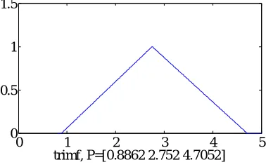
So here we get for first rule triangular membership function as
0 20 40 60
0 0.1 0.2
Generation
F
it
n
e
ss
v
a
lu
e
Figure 6. First membership function
Second membership function we can get as Range for b= x(2)=[0.8862 1.8191] And range for x= x(1)=[1.8192 2.7520]
Figure 7. Second membership function
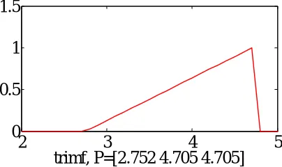
And third membership function as
Figure 8. Third membership function
0 1 2 3
0 0.5 1 1.5
trimf, P=[0.866 0.866 2.752]
2 3 4 5
0 0.5 1 1.5
trimf, P=[2.752 4.7052 4.7052]
0 1 2 3 4 5
0 0.5 1 1.5
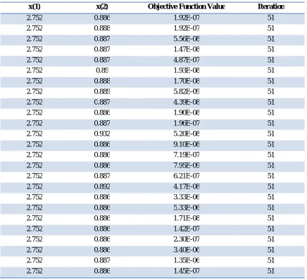
This result is for first run of the simulation so we run the simulation for 25 times and check the results for membership functions.
x(1) x(2) Objective Function Value Iteration
2.752 0.886 1.92E-07 51
2.752 0.888 1.92E-07 51
2.752 0.887 5.56E-08 51
2.752 0.887 1.47E-08 51
2.752 0.887 4.87E-07 51
2.752 0.89 1.93E-08 51
2.752 0.888 1.70E-08 51
2.752 0.889 5.82E-09 51
2.752 0.887 4.39E-08 51
2.752 0.886 1.90E-08 51
2.752 0.887 1.96E-07 51
2.752 0.932 5.20E-08 51
2.752 0.886 9.10E-08 51
2.752 0.886 7.19E-07 51
2.752 0.886 7.95E-09 51
2.752 0.887 6.21E-07 51
2.752 0.892 4.17E-08 51
2.752 0.886 3.33E-06 51
2.752 0.886 5.33E-06 51
2.752 0.886 1.71E-08 51
2.752 0.886 1.42E-07 51
2.752 0.886 2.30E-07 51
2.752 0.886 3.40E-06 51
2.752 0.887 1.35E-06 51
2.752 0.886 1.45E-07 51
Figure 9. Base values of first membership function with consecutive 25 run
Figure 10. Base values bar chart of first membership function with consecutive 25 run
Base values of second membership function with consecutive 25 run is shown in fig.6.10
x(1) x(2) Objective Function Value Iteration
2.752 4.705 5.12E-05 51
2.752 4.705 5.12E-05 51
2.752 4.611 5.38E-05 51
2.752 4.62 5.35E-05 51
2.752 4.698 5.14E-05 51
2.752 4.699 5.14E-05 51
2.752 4.578 5.48E-05 51
2.752 4.705 5.12E-05 51
2.752 4.661 5.24E-05 51
2.752 4.699 5.14E-05 51
2.752 4.315 6.40E-05 51
2.752 4.705 5.12E-05 51
2.752 4.605 5.40E-05 51
2.752 4.27 6.59E-05 51
2.752 4.703 5.13E-05 51
2.752 4.679 5.19E-05 51
2.752 4.705 5.12E-05 51
2.752 4.663 5.23E-05 51
2.752 4.705 5.12E-05 51
2.752 4.694 5.15E-05 51
0.882 0.883 0.884 0.885 0.886 0.887 0.888 0.889
2.752 4.642 5.29E-05 51
2.752 4.661 5.24E-05 51
2.752 4.565 5.52E-05 51
2.752 4.7 5.13E-05 51
2.752 4.668 5.22E-05 51
Figure 11. Base values of second membership function with consecutive 25 run
Below we show bar plot of 25 consecutive runs in which we get 4.70 repeating more time or maximum hits occurs at 4.70 so we consider that point as our base value.
For first membership function we get base values as follow
Figure 12. Base values bar chart of second membership function with consecutive 25 run
0 1 2 3
0 0.5 1 1.5
trimf, P=[0.866 0.866 2.752]
4 4.1 4.2 4.3 4.4 4.5 4.6 4.7 4.8
With this run we get one membership function which is repeated many times.
For second membership function we get base values as follow
And third membership function base values are as follow
So overall membership function we will get as follow
Figure 13. Overall membership function
We choose the overallMembership Function as shown in F A. Simulation And Result
The SIMULINK model of the Continuously Stirred Tank Reactor (CSTR) is simulated in MATLAB/SIMULINK environment. The simulation results for different cases using SIMULINK block diagram are given below.
2
3
4
5
0
0.5
1
1.5
trimf, P=[2.752 4.705 4.705]
0
2
4
6
0
0.5
1
1.5
trimf, P=[0.866 2.752 4.705]
0 1 2 3 4 5
1)
Case-1: When Time Delay is zeroTime Delay = 0, Desired operating Point ( )= (0.4472, 2.7520), Initial Conditions ( ) = (0.4, 2.5).
Here in the result open loop response with time delay=0 (fig. 11a) system response is not reaching to the desired operating point (0.4472, 2.7520). Working in closed loop manner (fig.11 b) it reaches to the On the other hand when system is desiredoperating point (0.4472,2.7520).
Figure 14. Simulation results CSTR when Time Delay is zero
2)
Case-2: When Time Delay is constantTime Delay = 0.5, Desired operating Pointx (t)= (0.4472, 2.7520), Initial Conditionsx (t) = (0.4, 2.5).
When system is having time delay but operates in open loopmanner system response (fig.12 c) is not reaching to thedesired operating point (0.4472, 2.7520). On the other hand when system is working in closed loop manner (fig.12 d) it reaches to the desired operating point (0.4472, 2.7520)
0 20 40 60 80 100
0 0.1 0.2 0.3 0.4
(a) open loop response, time delay=0
time st at e X1 X2/10
0 20 40 60 80 100
0.2 0.25 0.3 0.35 0.4 0.45 time st at e
(b) closed loop response, time delay=0
X1 X2/10
0 20 40 60 80 100
0 0.1 0.2 0.3 0.4 time st at e
(c) open loop response, x0=(0.4, 2.5)
Figure 15. Simulation results CSTR when Time Delay is constant
V. CONCLUSION
Stability analysis and design method for a class of nonlinear Time-Delay systems based on T-S fuzzy modeling and control approach is simulated. First, TS fuzzy models with time delay are extended to describe the nonlinear Time-delay systemuncertain nonlinear function. The design methodology is illustrated by application to the stabilization problem of a CSTR example, which is a classical nonlinear Time-Delay system.In this paper, T-S fuzzy approach is used to control nonlinear time delayed system and rules are optimized with the help of genetic algorithm approach. The system is operated in this system in open loop and close loop mode.The results are shown for different initial conditions.
REFERENCES
[1] Y. Cao and P. Frank, “Analysis and synthesis of nonlinear time-delay systems via fuzzy control approach,” IEEE Trans. Fuzzy Syst., vol. 8, no. 2, pp. 200–211, Apr.
[2] J. P. Richard, “Time-delay systems: An overview of some recent advances and open problems,” Automatica, vol. 39, no. 10, pp. 1667–1694, 2003.
[3] Y. He, M. Wu, J. She, and G. Liu, “Parameter-dependent Lyapunov functional for stability of time-delay systems with polytopic-type uncertainties,” IEEE Trans. Autom. Control, vol. 49, no. 5, pp. 828–832, May 2004.
[4] Slotine, Weiping Li, Applied Nonlinear Control. New Jersy, Prentice Hall, 1991.
[5] W. Assawinchaichote, S. K. Nguang, and P. Shi, Fuzzy Control and Filter Design forUncertain Fuzzy Systems. Berlin,Germany: Springer-Verlag,2006.
[6] M. S. Mahmoud and N. F. Al-Muthairi, “Design of robust controllers for time-delay systems,” IEEE Trans. Automat. Contr., vol. 39, pp. 995–999, Dec. 1994.
[7] G. Feng, “A survey on analysis and design of model-based fuzzy control systems,” IEEE Trans. Fuzzy Syst., vol. 14, no. 5, pp. 676–697, Oct. 2006.
[8] T. Takagi and M. Sugeno, “Fuzzy identification of systems and its applications to modeling and control,” IEEE Trans. Syst., Man, Cybern., vol. SMC-15, no. 1, pp. 116–132, Jan. 1985.
[9] B. Kosko, “Fuzzy systems as universal approximators,” IEEE Trans. Comput., vol. 43, no. 11, pp. 1329–1333, Nov. 1994. [10] .2000K. Gu, V. L. Kharitonov, and J. Chen, Stability of Time-Delay Systems. Berlin, Germany: Birkhauser, 2003.
[11] C. Hua, X. Guan, and P. Shi, “Robust stabilization of a class of nonlinear time-delay systems,” Appl. Math. Comput., vol. 155, no. 3, pp. 737–752, 2004.
[12] C. Hua, X. Guan, and P. Shi, “Robust backstepping control for a class of time delayed systems,” IEEE Trans. Autom. Control, vol. 50, no. 6, pp. 894–899, Jun.2005.
[13] X. Guan and C. Chen, “Delay-dependent guaranteed cost control for T–S fuzzy systems with time delays,” IEEE Trans. Fuzzy Syst., vol. 12, no. 2, pp. 236–249, Apr. 2004.
[14] X. Guan and C. Chen, “Delay-dependent guaranteed cost control for T–S fuzzy systems with time delays,” IEEE Trans. Fuzzy Syst., vol. 12, no. 2, pp. 236–249, Apr. 2004.
[15] C. Lin, Q. Wang, and T. Lee, “Stabilization of uncertain fuzzy time-delay systems via variable structure control approach,” IEEE Trans. Fuzzy Syst., vol. 13, no. 6, pp. 787– 798, Dec. 2005.
[16] F. Gouaibaut, Y. Blanco, and J. P. Richard, “Robust sliding mode control of non-linear systems with delay: A design via polytopic formulation,” Int. J. Control,vol.77,no.2,pp.206–215,2004
[17] M. S. Mahmoud and P. Shi, Methodologies for Control of Jump Time-Delay Systems. Boston, MA: Kluwer, 2003.
[18] W. Assawinchai chote, S. K. Nguang, and P. Shi, Fuzzy Control and Filter Design for Uncertain Fuzzy Systems. Berlin, Germany: Springer-Verlag, 2006
[19] Huai-Xiang Zhang, Feng Wang, Bo Zhang “Genetic Optimization Of Fuzzy Membership Functions”, Proceedings of the 2009 International Conference on Wavelet Analysis and Pattern Recognition, Baoding, 12-15 July 2009
0 20 40 60 80 100
0.2 0.25 0.3 0.35 0.4 0.45 time st at e
(d) closed loop response, x0=(0.4, 2.5)