www.atmos-meas-tech.net/8/875/2015/ doi:10.5194/amt-8-875-2015
© Author(s) 2015. CC Attribution 3.0 License.
Development of a sky imaging system for short-term solar
power forecasting
B. Urquhart, B. Kurtz, E. Dahlin, M. Ghonima, J. E. Shields, and J. Kleissl University of California, San Diego, California, USA
Correspondence to: B. Urquhart ([email protected])
Received: 27 February 2014 – Published in Atmos. Meas. Tech. Discuss.: 19 May 2014 Revised: 29 October 2014 – Accepted: 9 January 2015 – Published: 20 February 2015
Abstract. To facilitate the development of solar power fore-casting algorithms based on ground-based visible wave-length remote sensing, we have developed a high dynamic range (HDR) camera system capable of providing hemi-spherical sky imagery from the circumsolar region to the horizon at a high spatial, temporal, and radiometric resolu-tion. The University of California, San Diego Sky Imager (USI) captures multispectral, 16 bit, HDR images as fast as every 1.3 s. This article discusses the system design and oper-ation in detail, provides a characterizoper-ation of the system dark response and photoresponse linearity, and presents a method to evaluate noise in high dynamic range imagery. The system is shown to have a radiometrically linear response to within 5 % in a designated operating region of the sensor. Noise for HDR imagery is shown to be very close to the fundamental shot noise limit. The complication of directly imaging the sun and the impact on solar power forecasting is also discussed. The USI has performed reliably in a hot, dry environment, a tropical coastal location, several temperate coastal locations, and in the great plains of the United States.
1 Introduction
Solar power output of an individual generator, or even a fleet of generators, will have some level of variability due to the nature of the input source of light from the sun. The source of short-term variability of irradiance at the earth’s surface is clouds and atmospheric particulates, which are generally not controllable. To reliably integrate increasing amounts of solar power into the electric grid, forecasting, storage, addi-tional transmission, and ancillary power generation services
will constitute a portfolio of solutions to counteract variabil-ity.
From a planning and operations perspective, grid operators require consumption and generation estimates from years to minutes ahead. On the scale of days to minutes, solar power output forecasts are provided by some combination of weather models and remote sensing of clouds, along with stochastic learning methods. Forecasting of solar radiation in the 0–30 min ahead time frame poses unique challenges. High resolution models reported for both satellite and numer-ical weather prediction can issue forecasts that have 5 min time steps for a one kilometer grid (Mathiesen et al., 2013; Perez et al., 2013), while the best operational models often have coarser resolutions in both space and time (Dupree et al., 2009; Rogers et al., 2012; Mathiesen and Kleissl, 2011). However, in numerical models, timing and/or positioning er-rors of clouds are inevitable, and for satellites, infrequent image capture and parallax effects can result in inaccurate georeferencing of clouds. These errors make it difficult to achieve an accurate, high resolution short term solar fore-cast. This motivates a need for other forecasting tools and observational methods.
This work describes the development of sky imaging hard-ware for short-term solar power forecasting at UCSD. The UCSD Sky Imager (USI) provides unique capabilities needed for forecasting research and applications. The goal of this ar-ticle is to provide details on the USI system, and report on its imaging performance so that other workers in this field may make more informed purchasing and design decisions. The remainder of Sect. 1 discusses hardware requirements for sky imaging, and reviews relevant sky imaging hardware presented in the literature. Specifics of the USI hardware de-velopment and system operations are covered in Sects. 2 and 3, respectively. The imaging performance of the USI is char-acterized in Sect. 4, and Sect. 5 presents deployments of the USI to date.
1.1 Imaging system considerations for solar forecasting Sky imagers were historically built for recording meteoro-logical conditions such as sky cover. For this purpose it is not critical to image the area directly around the sun, so many systems have sun occluding devices to prevent direct sunlight from entering the optics. When the sun is unobstructed, more than 90 % of the photons entering the optics can come from the direct solar beam. For most camera systems, the hand-ful of pixels encompassing the sun saturate and thus direct-beam signal intensity is only known to exceed the saturation threshold. Immediately outside the direct beam is a region of intense forward scattering. Aerosols and dust scatter the di-rect beam predominantly in the forward didi-rection, increasing the size of region around the sun that will potentially saturate in a sky image. Cloud droplets and ice crystals, when present, also predominantly scatter in the forward direction and, de-pending on the scattered intensity reaching the camera, can further extend the size of the region that will saturate. Ob-taining on scale image information about the region around the sun requires appropriate imaging hardware and methods, especially when the region around the sun has a very high intensity. Further, this high intensity region can cause image quality degradation through internal reflections, diffraction caused by the aperture, sensor saturation, smear and bloom-ing, and, potentially, sensor damage (see Sect. 4.7 for further discussion relating to the USI). The significance of each of these potential issues is imaging system dependent.
The use of occluding devices eliminates many of these po-tential issues, which is why they are often adopted. Blocking the sun and the surrounding area, however, eliminates im-portant sky condition information needed to provide reliable forecasts in the first few minutes (<5 min) of the forecast period. If the occluding device obstructed a minimal amount of the image along with precision-positioning mechanisms, it could then be used without adversely affecting immediate-term forecast accuracy. For cost and reliability reasons, these requirements are difficult to achieve in practice. The TSI, for example, has a shadow band that occludes 14 % of the sky hemisphere, always in the region near the sun. Even for a
1.3 km2solar power plant, the shadow band on the TSI has
been demonstrated to obscure sky condition information for over half of the plant (Urquhart et al., 2013). With proper design, and appropriate image capture and correction algo-rithms, sky imaging systems can acquire atmospheric infor-mation from an appreciable amount of the region around the sun (e.g., Stumpfel et al., 2004). To this end, the high dy-namic range imaging method described in Sect. 4.5 provides a simple and robust approach.
The spectral content of the sky scene provides important information for the remote sensing of clouds and water va-por. Most camera systems capture visible wavelength im-agery that spans between 350 and 800 nm. This allows the measurement of shortwave solar radiation that is scattered by the clouds, atmospheric gases and aerosols. Silicon-based image sensors used in visible wavelength cameras are also sensitive up to 1.1 µm in the near infrared. The sixteen bit (or higher) versions of these, with a set of selectable band-pass and neutral density filters, can be used for enhanced day and nighttime cloud detection (Shields et al., 2013). Long-wave infrared (LWIR) imaging in the 8–13 µm range mea-sures cloud brightness temperatures which can be used to segment different cloud layers, estimate cloud heights, and potentially determine optical depth. LWIR imaging hardware costs significantly more than common visible wavelength imaging hardware, and it may not be practical for widespread deployment.
The image formation process in a sky imaging camera redirects radiant energy from the sky hemisphere onto the two dimensional image plane. Geometric and radiometric calibrations turn the brightness information at a given pixel position into a measurement of sky radiance at a given look angle. Geometric calibration relates a pixel position on the sensor array to a set of angles (azimuth and zenith) in a de-fined world coordinate system. This is a necessary step to accurately geolocate clouds. Solar forecasting methods such as Chow et al. (2011) and Yang et al. (2014) require geo-metric calibration of the imager because cloud positions are explicitly computed. Time of arrival methods such as Mar-quez and Coimbra (2013) or Wood-Bradley et al. (2012) do not require geometric calibration because only a forecast of when a cloud will occlude the sun for the location of the im-ager is needed. A treatment of geometric camera calibration is beyond the scope of this article, but the interested reader is referred to Faugeras (1993) or Hartley and Zisserman (2004) for an introduction to the calibration process, and Urquhart et al. (2015) for more on the geometric calibration of the USI. Radiometric calibration makes it possible to determine the radiance of the scattered light coming from a portion of the sky (Shields et al., 1998a; Feister and Shields, 2005; Román et al., 2012), and can be used as input to retrieval algorithms for a number of optical properties of atmospheric aerosols that impact solar energy generation (Nakajima et al., 1996).
The size (i.e., area) of a cloud element Acld (m2)observed
by a single pixel at a cloud heightH can be described as Acld=π H2sec2(θ )tan2(α) ,
whereθis the angle from the optical axis, andαdefines the field of view of the pixel. It has been assumed for simplicity that the field of view is a circular cone withαrepresenting the cone half-angle, with the cloud element orthogonal to the cone axis The solid angle subtended by the cone, and thus the pixel, is then 2π (1−cosα). For an equisolid angle lens (Sect. 2.1) α is nominally constant over the entire field of view, andAcldis a function ofθonly. If the patch of cloud is
projected to a plane parallel to the ground (Chow et al., 2011; Urquhart et al., 2013; Yang et al., 2014), for smallαthe area of the patch can be approximated as
Scld=
1 2π H
2sec(θ )tan(α) (tan(θ+α)−tan(θ−α)) .
If this cloud element is projected onto the surface as a “cloud shadow”, the area is approximately Scld when ignoring
ef-fects due to terrain. For an equisolid angle lens, the value of αis related to the pixel density as
α=acos 1−1/npix
, (1)
wherenpixis the number of pixels occupying the image of
the sky (assumed to be a 2π steradian hemisphere). Asnpix
increases,αdecreases, and thus the areasAcld andScld
de-crease, i.e., the resolving power of the system increases (as-suming the lens is not the limiting factor). Atθ=30◦,Acld
for the TSI (npix≈0.14 Mpixels) is 544 m2at a 3 km cloud
height, whereas for the USI (npix≈2.32 Mpixels) it is 33 m2.
ForScld, the corresponding values are 1257 and 75 m2,
re-spectively. If a pixel is incorrectly labeled a cloud (or as clear), it has a much larger areal impact for the TSI than for the USI.
1.2 Existing sky imaging hardware
There are three fields where a majority of sky imaging work has been performed: atmospheric sciences, forestry and ecol-ogy, and astronomy. Camera developers in astronomy are typically concerned with having a high sensitivity and low noise so that a high percentage of incoming photons from stars, asteroids and other faint objects are converted into charge carriers on the image sensor. The sensors used are of-ten full frame charge-coupled devices (CCDs) because of the high quantum efficiency and fill factor, but require mechani-cal shuttering which limits the frame rate of the system. One system similar to the USI from the astronomy field is the All Sky Infrared Visible Analyzer (ASIVA, Klebe et al., 2014; Sebag et al., 2008) with a dual camera system that captures both visible and LWIR images. It is one of the few LWIR dioptric (refraction-based) whole-sky designs (catadioptric (reflection and refraction) designs similar to the TSI are more
common). It uses a 640×512 uncooled microbolometer ar-ray sensitive in the 8–13 µm range with a germanium fish-eye lens. The system has an 8-slot filter wheel allowing for multiband LWIR measurements. The ASIVA also has a high-resolution visible camera with an 8-slot filter wheel (specific camera model has varied by ASIVA unit).
The area of forestry has extensively used hemispheri-cal photography (Brown, 1962; Anderson, 1964). The high-dynamic-range all-sky-imaging system (HDR-ASIS) is a CMOS-based camera that leverages multiple exposures to create a high-dynamic-range (HDR) composite sky image for ecosystem and canopy research (Dye, 2012).
Researchers in atmospheric science have very actively developed their own instruments over the years. In fact, Hill (1924) mentions cloud photography as a motivation in developing the first true fisheye lens design. Digital sky pho-tography began in the 1980s with the development of per-sonal computers, and one of the leading groups developing imaging systems for atmospheric observation was the Atmo-spheric Optics Group at the Scripps Institute of Oceanog-raphy’s (SIO’s) Marine Physical Laboratory (Johnson et al., 1988, 1989). Their well known Whole Sky Imager (WSI) is still to this day one of the highest quality, if not the highest quality, sky imaging systems ever developed (Shields et al., 1998b, 2013). It was developed primarily for US military ap-plications in the 1980s and early 1990s. More recent designs of the system had a 512×512-pixel temperature-controlled, 16-bit low-noise monochrome CCD camera. It used a Nikon Nikkor 8f/2.8 (8 mm) fisheye lens (equidistant projection, Sect. 2.1) and two filter wheels holding neutral density and spectral filters at multiple wavelengths. The image plane was the surface of a tapered fiber-optic bundle that interfaced di-rectly to the CCD. Multiple corrections were made to the instrument to improve measurement quality: dark field rection; flat field correction (among other things, this cor-rected imaging issues caused by fiber optic imperfections); exposure corrections; linearity corrections; roll-off correc-tions; geometric calibration; and in some cases absolute ra-diometric calibration. By adjusting the neutral density and spectral filter selections, and/or the exposure time, the system achieved a wide dynamic range and could capture both day-time and nightday-time imagery with high accuracy. The cloud detection algorithms developed over several decades were sophisticated, with accurate detection of haze, thin cloud, and opaque cloud (Shields et al., 1993a, b, 1998a; Feister and Shields, 2005).
37 1
2
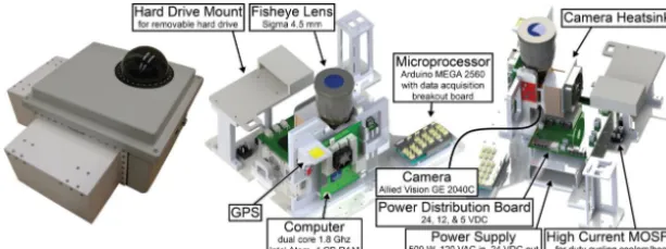
Fig. 1. The UCSD Sky Imager enclosure (left) and a CAD model showing the layout 3
of system components (right).. 4
5
Figure 1. The UCSD Sky Imager enclosure (left) and a CAD model showing the layout of system components (right).
8 bits), and there is little control of the camera capture set-tings. An antireflective black rubber strip (“shadow band”) affixed to the mirror prevents direct sunlight from reflect-ing into the camera optics which improves image quality and avoids damage to the sensor. The shadow band covers approximately 0.70 steradians of the hemisphere, which is about 14 % of the image region used for forecasting (<80◦ zenith angle). Accurate geometric calibration of the TSI is challenging because of the mirror design. Translation and ro-tation of the mirror with respect to the camera body (the cam-era is understandably not perfectly over the mirror center) makes modeling the camera geometry more complicated and thus calibration is more challenging than for upward point-ing systems with a spoint-ingle lens. Additionally, the mirror is often slightly warped in shape (i.e., not perfectly spherical), and the surface is covered in small scale imperfections that produce local distortion. A comparison of the solar forecast-ing performance between the TSI and USI was performed by Gohari et al. (2014).
Beyond the WSI and TSI, a number of other imaging sys-tems have been developed for atmospheric studies. A de-scription of several of these can be found in Urquhart et al. (2013) and in Table 1. Outside of systems developed by research groups, there are alternatives to the TSI. The SONA (Sistema Automático de Observación de Nubes, Gonzales et al., 2012) uses a 1/300, 640×480 CCD, has integrated coolers, heaters and temperature sensors and is ruggedized for outdoor deployment. It has an integrated shadow band with azimuth control that shades part of the lens, but not the full optical system (i.e., it does not shade the entire dome). The Eko sky camera, built by Schreder, is reported to have 2 Mpixels, and like the SONA and TSI, has cloud detection software and a user interface. The Santa Barbara Instrument Group (SBIG) sells the Allsky-340C camera system based on a Truesense KAI-0340, 640×480 CCD with a speci-fied dynamic range (defined Sect. 2.2) of up 69 dB, and uses a 1.4 mm focal length Fujinon FE185C046HA-1 lens. The SBIG camera was used for solar forecasting research by Fu and Cheng (2013). Inclusion of a sky camera in this discus-sion is not meant to indicate it is not suitable for solar power forecasting. The list of systems noted here is far from
com-prehensive, and with the potential of sky imagery for solar energy applications, new systems are continuously being de-veloped.
2 Hardware design and selection methods 2.1 Optical design
The University of California, San Diego has developed its own sky imager (the USI, Fig. 1) to address the instrument needs for short term forecasting. The USI uses a Sigma 4.5 mm focal length fisheye lens which allows the entire im-age circle to fit on the sensor. This can easily be verified from the focal length, the lens projection, and sensor size. A con-ventional camera lens has the rectilinear projection function rs =ftan(θ ) ,
wheref is the focal length,θ is the angle from the optical axis, andrsis the distance from the principal point in the im-age plane. It is evident that this pinhole camera model cannot image points at 90◦from the optical axis with a sensor of fi-nite size. In order to form the image of points that are 90◦ from the optical axis within a finite image plane, distortion is required, and the type of distortion can be selected by the optical designer. The two most common projections used in fisheye lenses are the equidistant and equisolid angle projec-tions,redandres, respectively:
red=f θ
res=2fsin
θ 2
.
Table 1. Research camera systems for sky atmospheric observations.
System Camera Sensor Resolution Lens Reference
WSI Photometrics S300 CCD 512×512 Nikon, equidistant Shields et al. (2013)
WSC – CCD, 1/300, 8.3 mm 752×582 1.6–3.4 mm Long et al. (2006)
ASI (GFAT) QImaging RETIGA 1300C Sony ICX085AK CCD, 2/300, 12-bit 1300×1030 Fujinon FE185C057HA Cazorla et al. (2008) Román et al. (2012)
IFM-GEOMAR – 10-bit 3648×2736 – Kalisch and Macke (2008)
ASI (CAS) – 1/300CCD 2272×1704 equidistant Huo and Lu (2012)
38 1
2
Fig. 2. (a) Perspective (rectilinear), equidistant, and equisolid angle projection 3
distances as a function of incidence angle, along with the projection for USI 1.2 4
determined from geometric calibration. The projection distance is normalized by the 5
focal length. (b) Zenith angle resolution of projections in (a). 6
7
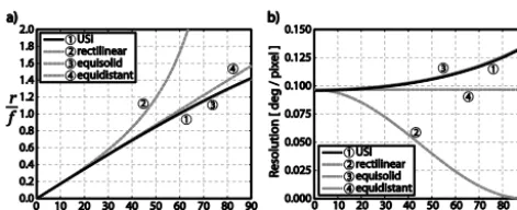
Figure 2. (a) Perspective (rectilinear), equidistant, and equisolid
an-gle projection distances as a function of incidence anan-gle, along with the projection for USI 1.2 determined from geometric calibration. The projection distance is normalized by the focal length. (b) Zenith angle resolution of projections in (a).
with that measured for the USI system. The angular resolu-tion per pixel is shown in Fig. 2b. Figure 2b assumes the sen-sor is 15.15 mm across containing 2048 pixels, and uses the specifications for USI 1.2 in Table 2. Even though the angu-lar resolution at the horizon is coarser for an equisolid versus an equidistant projection at the same focal length, the for-mer was selected for the USI because at large zenith angles, the horizontal configuration of clouds is difficult to determine because of self occlusion and perspective effects. Using more of the sensor area for the sky region overhead and near the sun (during midday) was preferred because these sky areas contain the clouds causing the current and near future solar power generation impacts when power output is highest.
For a given sensor size, the selected projection places a limit on the maximum allowable focal length of a lens while still being able to capture the complete sky dome (or con-versely, the minimum sensor size given a focal length). The maximum allowable focal length for the equidistant projec-tionfed,maxis 2rmin/πand for the equisolid angle projection
fes,maxisrmin/ √
2, whererminis the shortest distance from
the principal point to the edge of the sensor. For the USI, with a sensor size of 15.15 mm, rmin is 7.575 mm
(assum-ing the principal point is in the center of the image sensor), and a focal length of less than 5.36 mm for the equisolid an-gle projection is required. Because the principal point will in general vary depending on machining and assembly tol-erances of the components used, the value ofrminwill vary.
Table 2 shows the principal point location, rmin, andfmax,
for several USI systems obtained from a nonlinear
geomet-Table 2. Intrinsic parameters and lens focal length selection
param-eters measured for 7 USI units. The principal point(uo, vo) and
focal lengthf are measured for each USI. The minimum distance to the sensor edgerminfrom(uo, vo)yields the maximum allowable
focal lengthsfed,maxandfes,maxfor the equidistant and equisolid
angle projections, respectively. Units are in mm, except foruoand vowhich are given in pixels.
USI no. uo vo f rmin fed,max fes,max
1.1 1032 965 4.437 7.139 4.545 5.048
1.2 1040 970 4.386 7.176 4.568 5.074
1.5 1033 963 4.429 7.124 4.535 5.037
1.6 1028 991 4.377 7.331 4.667 5.184
1.8 1023 1043 4.448 7.434 4.733 5.257
1.9 1045 976 4.474 7.220 4.596 5.105
mean 1033.5 984.7 4.425 7.237 4.607 5.118
SD 7.3 27.7 0.034 0.111 0.071 0.079
ric calibration of extrinsic and intrinsic parameters that min-imized the squared pixel error between actual sun position measurements and modeled sun position. The NREL solar position algorithm (Reda and Andreas, 2004) was used for modeled sun position input. The principal point shows sig-nificant variation because the mounting location of the lens fluctuates by as much as 0.31 mm. As a result, the radial dis-tance to the edge of the detector fluctuates, and along with it the maximum allowable focal length.
39 1
2
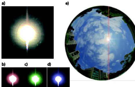
Fig. 3. (a) Diffraction pattern measured with a 1000 µm aperture on USI 1.8, with
3
color red, green, and blue color components shown in (b), (c), and (d), respectively. 4
(e) Diffraction of the hexagonal iris blades in the stock lens. 5
6
Figure 3. (a) Diffraction pattern measured with a 1000 µm
aper-ture on USI 1.8, with red, green, and blue color components shown in (b), (c), and (d), respectively. (e) Diffraction of the hexagonal iris blades in the stock lens.
circular apertures of diameter 300, 700, and 1000 µm (Fig. 3). Because diffraction caused by a circular aperture generates a known Airy disk pattern, it is possible to partially correct the image with deconvolution processing, however this was not done in this work. To minimize the incoming flux while also minimizing diffraction, an aperture of 1250 µm was selected. In comparison, the aperture diameter with the ND filter is 9520 µm. This large diameter noticeably reduces the depth of focus of the camera compared to the 1250 µm aperture (depth of field is unaffected because a fisheye lens is used). The ra-diant flux is higher using an aperture of 1250 µm compared to the ND filter configuration by a factor of 18. This allows shorter exposures with less motion blur caused by longer in-tegration times, but may also lead to increased sensor degra-dation in the long term due to the increased radiation on the sensor.
In order to develop a ruggedized system, it is necessary to protect the lens and properly seal the enclosure from the en-vironment. For the lens to have full 180◦access to the sky with this requirement, a 1/16th inch thick, neutral density acrylic dome was used on the USI. The dome has a UV hard-coat applied to minimize transmission of high energy solar radiation which helps reduce component degradation. Amor-phous silicate glass has superior transmissivity and scratch resistance than acrylic, but is more difficult to machine and handle, and designing proper sealing for a glass dome is more complicated (and thus more expensive). Polycarbonate, while having similar transparency and machining character-istics to acrylic, becomes opaque due to oxidation, making it a poor choice as a dome material (stabilizer additives can dramatically improve the lifetime). A drawback of acrylic is that it is susceptible to scratching from wind-blown partic-ulates (common in the desert), improper cleaning, and birds which occasionally land on the dome and scratch it with their talons or beak. The use of a neutral density acrylic dome with
a higher neutral density and an anti-reflective coating on the inner surface is being considered to improve image quality further.
2.2 Camera and image sensor
The USI uses an Allied Vision GE-2040C camera which contains a 15.15×15.15 mm, 2048×2048 pixel Truesense KAI-04022 interline transfer CCD sensor. The camera is connected to the computer with a gigabit ethernet interface, and customized control is achieved by using the PvAPI for Linux provided by Allied Vision. For solar forecasting re-search, we have found that the ability to adjust exposure in-tegration times, frame rates, regions-of-interest, and other pa-rameters is a necessary capability.
The USI imaging system was designed to generate images suitable for cloud detection and motion processing. Cloud detection requires spectral measurements, and thus a spectral filtering method must be employed in some capacity. Cou-pled with a high quality sensor, camera, and lens, a mechani-cal shutter and color filter wheel can provide very high qual-ity still spectral measurements. These moving components, however, complicate system design and HDR capture, and limit frame rates, therefore no mechanical shutter or color filter wheel were used. Spectral measurements were instead obtained by using a sensor with Bayer color filter array (CFA, Bayer, 1975).
The intensity range of the sky necessitates a sensor with a large dynamic range. Large dynamic range and global elec-tronic shuttering are available from interline transfer CCDs, which is why this technology was selected for the USI. Dy-namic range DR is defined by the ratio of maximum measur-able signal to the noise floor:
DR=20log10csat crd
,
wherecsatis the count value at saturation andcrdis the read
noise. For a single USI exposure,csatis 4095 counts andcrd
exposure which is not rescaled, and thus for the USI with csat=65 535 this gives 84 dB. This is somewhat misleading,
however, because rescaling the shorter exposures decreases signal-to-noise ratio by up to a factor of 4 (when the only the shortest exposure is used). Therefore, while the improved dy-namic range from HDR imaging can better capture the wide intensity range of the sky, it comes at a cost of increased noise for darker pixels.
The use of an interline transfer CCD is not without trade-offs. Smear is very apparent in images with direct sun ex-posure. Smear has two sources: (1) stray light entering the VCCD (vertical transfer CCD) during readout; (2) charge generation occurring deeper in the silicon photodiode layer that diffuses to any of the charge collection or transfer elec-tronics. The VCCD is the interline column near the exposed photodiode column, and is where the vertical readout step is performed. Longer wavelengths penetrate further into the silicon before being absorbed and can generate hole–electron pairs in undesirable locations. This is why the smear is no-ticeably worse in the red channel of Fig. 3b. Blooming, which is apparent as a saturated border of bright objects, is another problem for CCDs, and is noticeable in USI imagery near the sun. It is not serious however, because each KAI-04022 pixel has a vertical overflow drain to prevent large amounts of charge from diffusing to nearby collection sites.
2.3 Enclosure and balance of system design
For solar forecasting, tough environmental conditions such as hot and dusty deserts will be encountered. The USI is de-signed to survive 60◦C ambient air temperature and direct sunlight conditions. It has a light-colored exterior to reduce shortwave absorption and has two 80 W thermoelectric cool-ers with a NEMA 4X rating. To monitor the system’s en-vironmental health, a suite of temperature and relative hu-midity sensors was added to measure camera, power supply, internal and external ambient, and dome conditions. The in-ternal enclosure walls are all insulated to reduce thermal con-ductivity of the enclosure, which with the use of active ther-mal control, keeps it cooler on hot days and warmer on cold days. Internal water condensation was initially found to be an issue. Improved system sealing and thorough water test-ing was found to be necessary. Three 20 W resistive heattest-ing strips were installed on the base of the dome to reduce con-densation on the exterior dome surface.
The USI camera is controlled by a 1.8 Ghz dual core (Atom D525) embedded computer running Linux Ubuntu 12.04. The images can be stored locally on a set of inter-nal and USB hard drives, or it can be transferred across a network connection. Using an embedded computer gives the system flexibility for customizing the configuration on a per deployment basis, and the capture software can easily be re-configured, reprogrammed, or debugged remotely. A labeled CAD model of the USI is shown in Fig. 1.
3 System operation
3.1 Image capture and storage
Images are received from the camera as uncompressed single-channel 12-bit images with per-pixel color determined by the CFA. After three exposures are composited in the HDR process (Sect. 4.5), the combined image is still a single channel, but with 16-bits per pixel. Images are compressed and stored in a lossless 16-bit PNG format as a single channel image. A single pixel contains information about only one color of red, green or blue light. To produce a full color image from the pixel array suitable for processing, linear demosaic-ing is applied prior to use. Current image sizes are around 3 MB per image, which when capturing images every 30 s during daylight hours requires between 3 and 6 GB day−1 de-pending on the time of year.
The maximum frame rate of the USI system in single
expo-sure mode is 15 fps, which is relatively low. Future dynamic
computer vision approaches to solar forecasting (e.g., optical flow) may require higher frame rates, and for these methods, the camera used on the USI may not be suitable. In HDR
mode, which is the standard USI operational mode, three
im-ages are captured sequentially in 160 ms, which is a frame rate of 18.8 fps (or HDR frame rate of 6.3 fps). This increase in frame rate is possible because a smaller 1748×1748 re-gion of interest, extracted from the center of the 2048×2048 pixel array, is transferred off the camera. After subsequent HDR compositing and PNG image compression, the effec-tive frame rate drops to 0.77 fps (i.e., 1.3 s per HDR image). 3.2 System monitoring and control
The raw images generated by the camera are inconvenient for qualitative inspection on a user’s screen because they are not in color (raw Bayer format), the file sizes are relatively large so loading is slow, and a majority of the sky resides within the lower end of the 16-bit dynamic range which means the im-age appears very dark except for the sun. Preview imim-ages are therefore generated, which are full color, but lower resolu-tion, compressed, and tone-mapped to 8 bits per color chan-nel. These previews are small enough to be uploaded to the operator from all sites – including remote ones using a cellu-lar modem – and allow the image quality and availability to be inspected at a glance.
backup, particularly on remote systems that are hard to ac-cess and crash more often than the others due to bugs in the cellular modem driver.
4 Imaging performance characterization 4.1 Noise sources and pixel photoresponse
Each pixel in a camera is an independent radiometric sen-sor, and has small response variations from its neighbors due to small manufacturing differences. After charge is collected on a pixel, it is converted to a voltage and then to a digital value, and at each step in the process noise is introduced. Common sources of noise include dark current generated by the semiconductor in the bulk and at the surface, reset noise from charge to voltage conversion (which is typically min-imized by correlated double sampling), read noise from the camera’s readout electronics, and photoresponse nonunifor-mity (PRNU) arising from small manufacturing differences of each pixel. Because there is a consistent spatial variation of many of these noise sources, it often forms a pattern called fixed pattern noise (FPN). Shot noise, arising from the quan-tum nature of the photons generating the signal, occurs in all imaging systems and acts as a lower bound to measurement uncertainty. It adds a random element to each image that is Poissonian in nature and it can only be reduced by averaging frames, which is not feasible for fast-moving clouds or when high frame rates are desired.
Each pixel’s response can be characterized and corrected so that under the same illumination, the corrected output is the same when averaged over several frames. A compari-son of the average of several frames is required because shot noise will always be present in an individual frame. A poly-nomial can be used to model a pixel’s response to light:
cij(I, t )= N X n=0 ˆ aij,ntn+
M X m=1
dij,m(I t )m, (2)
wherecij(I, t )is the camera measurement in counts at thei, j pixel location,Iis the irradiance incident on the pixel,tis the integration time of the exposure,aˆij,nare coefficients that characterize the individual pixels’ dark response, and dij,m characterize the pixels’ photoresponse. Sensor noise and re-sponse characteristics are temperature dependent, so coeffi-cientsaˆij,n, anddij,mwill also vary with temperature. Here it has been assumed that dark response and photoresponse can be separated.
To determine the coefficients in Eq. (1), the irradiance I on the sensor plane must be known, which when using a lens implies the scene radiance must be known over the entire field of view. This can be achieved with a calibrated flat-field source. Many of the components of solar forecasting algo-rithms (e.g., Chow et al., 2011; Yang et al., 2014) have a training step where either relative brightness or brightness ra-tios are used to determine thresholds, or texture information
is used and therefore calibrated radiance is not needed. In-stead, these algorithms require spatially consistent measure-ments (i.e., consistent between pixels), for which a simpler radiometric uniformity correction (Sect. 4.3) can be used. This has the advantage that it can also be employed in the field after the instrument has been deployed. The camera out-put signalsij after radiometric uniformity correction can be written as:
sij(I, t )= M X m=0
bij,m cij(I, t )−aij(t ) m
, (3)
whereaij(t )provides the dark-field correction, and coeffi-cientsbij,mprovide the flat-field (i.e., uniform illumination) correction.
The parameters of the radiometric uniformity correction aij and bij,m have temperature dependencies that are not treated in the formulation of Eq. (2) or developments to fol-low. Sky imaging systems expecting large changes in sen-sor and camera temperature should perform the testing de-scribed in Sects. 4.2–4.4 at different temperatures to better understand the impacts. For the USI, the dark current of KAI-04022 roughly doubles for every 9◦C increase in temperature in the system operating range. The USI camera temperature, measured with an LM335 thermal probe attached to the cam-era body, has been observed to change by over 20◦C between day and night.
4.2 Dark response
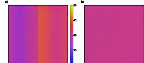
40 1
2
Fig. 4. (a) Occurrence frequency of signal measured in a dark room for 25 different 3
integration times, ranging from 1ms (black) to 2s (lightest gray). Ten exposures at 4
each integration time were averaged to construct each histogram. (b) Occurrence 5
frequency of the signal in a single frame for the 25 integration times with an average 6
1ms frame subtracted. Individual labels for each integration time were not added 7
because curves are not discernable. 8
9
Figure 4. (a) Occurrence frequency of signal measured in a dark
room for 25 different integration times, ranging from 1 ms (black) to 2 s (lightest gray). Ten exposures at each integration time were averaged to construct each PDF. (b) Occurrence frequency of the signal in a single frame for the 25 integration times with an average 1ms frame subtracted. Individual labels for each integration time were not added because curves are not discernable.
The temporal component of the dark response for the ex-posure times used on the USI (<1 s) is small, but there is still a spatial component of the dark response called fixed pattern noise (FPN). The FPN is shown in Fig. 5a. There is rela-tively little variation within each column. Two distinct image halves are noticeable, an artifact caused by the use of two A/D converters, each serving half the sensor. Columns near the center of each half have lower readouts than columns near the edges. The dark FPN can be removed by subtracting the measured dark response to obtain the dark field corrected sig-nalsijd(I, t )
sijd(I, t )=cij(I, t )−aij(t ) , (4) which is the same as the term in parenthesis in Eq. (1). The dark image termaij(t )is obtained by averaging several frames at integration timet. An image appears much more uniform after dark correction (Fig. 5b) which indicates the FPN has been eliminated. For over 99.9 % of pixels,aij(t ) does not show significant variation with time, however a small number of “hot” pixels have higher than average dark current and/or a nonlinear temporal dark response, and thus the time dependence ofaijis retained.
4.3 Sensor photoresponse uniformity correction Photoresponse nonuniformity is caused by differing gains on each photodetector in the focal plane array; i.e., dij,m in Eq. (2) differs slightly for each pixel. The most direct approach to PRNU correction uses flat-field measurements (uniform lighting over the entire field of view) in order to ad-just each pixel so that its response is uniform under uniform illumination. An alternative method is to use an illumination source that produces a smooth image without large bright-ness gradients. The resulting image can then be fit with a sur-face, and deviations of a given pixel from this surface can be considered the non-uniformity of that pixel. At each integra-tion time, 10 exposures are used to obtain an average of the dark corrected signalsijd(I, t )so that the effects of shot noise
41 1
2
Fig. 5. (a) An example dark frame for a 100ms exposure and (b) the corrected dark 3
frame. Typical pixel values in (a) range from 32 to 47 with a mean around 40 counts 4
(of 212). 5
6
Figure 5. (a) An example dark frame for a 100 ms exposure and (b) the corrected dark frame. Typical pixel values in (a) range from
32 to 47 with a mean around 40 counts (of 212).
are reduced (the 10-frame average denoted bysijd(I, t )). The same integration times used for the characterizing the dark response in Sect. 4.2 are used. At each integration time, a 5th order surface (denotedhsijd(I, t )i) is then fit to the aver-age dark corrected signalsijd(I, t )as a function of pixel loca-tion (iandj ). The resulting set of surfaceshsijd(I, t )iis used to determine the coefficientsbij,mas a function of exposure timet:
hsijd(I, t )i =
M X m=0
bij,m
sijd(I, t )m, (5)
where for each pixelij, bothsijd(I, t )andhsijd(I, t )iare a function of position(i, j )and exposure time (here we assume the scene brightness is not changing, thusI is constant). The surface fit also assumes that if a CFA sensor is used, separate surface fits are used for each color channel. Before fitting a surface tosijd(I, t )(Fig. 6c) at each integration time, a row-by-row adjustment was applied to remove the imbalance in output from the A/D converters. A low-order fit of the row-by-row ratio of two columns on either side of the border be-tween image halves was used to adjust the left side of the image.
42 1
2
Fig. 6. (a) Raw red image of smooth light source obtained by sub-sampling only red 3
pixels from the color filter array; (b) average of ten red frames, including (a); (c),(d) 4
uniformity correction applied to (a),(b), respectively. 5
6
Figure 6. (a) Raw red image of smooth light source obtained by
sub-sampling only red pixels from the color filter array; (b) average of ten red frames, including (a); (c, d) uniformity correction applied to (a, b), respectively.
4.4 Photoresponse linearity
Knowledge of the camera’s response as a function of both intensity and exposure time is a prerequisite for the HDR process. The simplest model for a pixel’s photoresponse is linear in the product of irradianceI on the sensor plane and exposure timet
cij(I, t )= ˆaij,o+dij,1I t, (6)
whereM andN from Eq. (1) have been taken as zero and one, respectively. Assuming a constant irradiance during the exposure sequence, we convert the value measured in an ex-posure of integration timetto the expected value had it been captured at integration timetref:
cij(I, tref)= cij(I, t )− ˆaij,o tref
t + ˆaij,o. (7)
This linear model predicts that the measurement values of the same scene should be scaled by the ratio of the exposure times from one image to the next. For example, we would ex-pect that all the values in a 6 ms exposure would be 4 times as large as the values of the corresponding pixels in a 1.5 ms ex-posure. Figure 7 shows the ratio of modeled values based on a longer exposure to the measured values in a shorter expo-sure (i.etref/t=0.25). An average of five frames was used at
each exposure time in making the comparison. To avoid neg-atively biasing the results, pixels that saturate in the longer image were removed, which corresponds to pixel values of over 1024 in the shorter exposure.
43 1
2
Fig. 7. Evaluation of sensor linearity using sky images under thin overcast conditions. 3
In (a), a point cloud (and median in red) showing the distribution of the ratio between 4
a 6 ms exposure and a modeled 6 ms exposure generated from a 1.5 ms exposure, 5
as a function of measured value in the 1.5 ms image. In (b), the same as (a), but with 6
6 ms and 24 ms exposures. In (c) the median line for each color is shown. To reduce 7
random noise, each of the compared images is the average of five exposures 8
captured over the course of approximately 3 seconds. 9
10
Figure 7. Evaluation of sensor linearity using sky images under thin
overcast conditions. In (a), a point cloud (and median in red) show-ing the distribution of the ratio between a 6 ms exposure and a mod-eled 6 ms exposure generated from a 1.5 ms exposure, as a function of measured value in the 1.5 ms image. In (b), the same as (a), but with 6 and 24 ms exposures. In (c) the median line for each color is shown. To reduce random noise, each of the compared images is the average of five exposures captured over the course of approximately 3 s.
The observed deviation from unity is a measure of the er-ror we introduce by scaling up a given value from the short exposure to place it in a composite with the longer expo-sure. Below 100 counts (∼2.5 % full scale), there appear to be significant non-linearity effects, and we do not recom-mend using signals below this level. Between about 400 and 800 counts, the median deviation is nearly zero. Deviations are small (<5 %) from around 150 counts to the end of the overlap range just above 1000 counts. Over the majority of the range, neither exposure time nor color has a significant effect on the result. The overlap of this “sufficiently linear” region on the abscissa of Fig. 7 extends from 409 counts (the lower limit in the short exposure) to 921 counts (the upper limit in the long exposure after multiplying by the integra-tion time ratio, i.e., 3684×0.25=921). We have therefore elected, for the purposes of this work, to consider pixel re-sponse to be sufficiently linear if the value is between 10 and 90 % of full scale, i.e., 409 to 3686 counts.
4.5 High dynamic range imaging
com-Figure 8. USI 1.2 high dynamic range (HDR) exposure sequence
for (a) 23 May 2013, 03:22 pm PDT and (b) 23 May 2013, 02:48 pm for integration times of (i) 30, (ii) 120, and (iii) 480 ms. (a-iv) and
(b-iv) show the final HDR composites.
bine those exposures into a single high dynamic range image (Debevec and Malik, 1997). Three 12-bit exposures are com-posited together to produce a single 16-bit image.
Although methods exist that would allow us to use a more sophisticated photoresponse model than Eq. (5) (e.g., Mann and Picard, 1994), by only using pixels in the linear region of the sensor photoresponse (Sect. 4.4), we can apply the simple linear response model without significant error. For purposes of the HDR composite, this means that for a single exposure the pixels with values below 409 or above 3686 counts are excluded. The integration times on the USI are separated by factors of four (i.e.,t, 4t, and 16t, wheretis system depen-dent). This ensures that the region between 409 and 921.5 counts in a shorter exposure will overlap with the region be-tween 1636 and 3686 counts in a longer exposure. Based on the results shown in Fig. 7, these settings ensure the linear approximation in Eq. (5) is applicable for the subset of over-lapping pixels in the HDR image.
The HDR process is straightforward. First we select the pixels in each of the three exposures that are properly ex-posed, eliminating areas that are below 10 or above 90 % of full scale. Next, using Eq. (6), we map the values for each pixel to what they would have been in the frame with the longest exposure time. This assumes that for the short dura-tion of an HDR exposure sequence, scene intensity is con-stant. Finally, we combine the exposures, using the average of all valid values for each pixel. This method is simple and effective, as demonstrated in Figs. 8 and 9. It is, however subject to small composition artifacts if the sensor response linearity is not properly characterized. If an image patch con-tains values for which sensor response is nonlinear and the HDR algorithm transitions from using a different subset of the three available exposures within this patch, a small 1– 2 pixel intensity step will occur which, after demosaicing into a color image, appears as a color fringe.
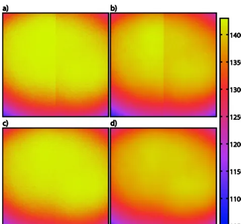
Figures 8 and 9 demonstrate the HDR method applied to two systems, USI 1.2 and USI 1.8 respectively (see Table 3). USI 1.2 used a 9520 µm diameter aperture and neutral density
Figure 9. HDR images from USI 1.8 in April and May 2013,
show-ing a variety of sky conditions. Images required intensity rescalshow-ing for display purposes.
filter, whereas USI 1.8 used a modified aperture of diameter 1000 µm (note the spectral variation between instruments). Figure 8a and b highlights the differences between the HDR capture sequence in cloudy conditions for an obstructed and unobstructed sun. Figure 9 provides an overview of imag-ing performance in a variety of sky conditions, with both ob-structed and unobob-structed sun. Figure 9d shows a thin cloud in low lighting conditions, and in Fig. 9g a halo caused by the thin clouds can be seen.
4.6 Brightness measurement uncertainty in HDR imagery
Two images of the exact same scene will not be identical due to the random shot noise present in the measurements. Electron generation in the sensor follows a Poisson distri-bution, so the root mean square (rms) of the shot noise is expected to beeij,shot=
√
eij, whereeij is the quantum unit being measured at pixeli,j. The quanta considered here is electrons. Assuming shot noise is the dominant noise source, this square root increase in rms shot noise with stored elec-tric chargeeijimplies the signal-to-noise ratio also increases as√eij. Shot noise places a fundamental limit on the lower bound of measurement uncertainty for an image sensor. The predicted rms noise as a function of count value for a 12-bit image is shown in Fig. 10a. For this calculation, the man-ufacturer specified gaing of 0.174 counts per electron was used. Measured system noise as a function of pixel value (in counts) was quantified by computing the pixel-by-pixel stan-dard deviationσij for ten frames of a stationary scene, bin-ningσij by the pixel-by-pixel meanµij into bins 0–4095, and finally by taking the medianσ of each bin. The drop-off near the maximum occurs because the upper bound that the saturation limit imposes causes the standard deviation of measured values to reduce.
When combining exposures in an HDR composite, the shot noise present in an individual pixel will depend on which exposures were compiled for that particular pixel, and the scaling factortref/tfor each pixel in the composition. For
distribu-Table 3. USI Locations in the United States and deployment time ranges.
USI no. Longitude (◦) Latitude (◦) Altitude (m) State City Start date Stop date 1.1 −117.233088 32.881090 120 California La Jolla 21 Apr 2012 – 1.2 −117.240987 32.872136 135 California La Jolla 6 Jun 2012 – 1.5 −117.243111 34.076355 347 California Redlands 18 Oct 2012 Mar 2014 1.6 −117.209333 34.079822 384 California Redlands 23 Oct 2012 Mar 2014 1.7 −97.478766 36.618377 304 Oklahoma Billings 11 Mar 2013 4 Nov 2013 1.8 −97.484871 36.604094 318 Oklahoma Billings 11 Mar 2013 4 Nov 2013 1.9 −117.238378 32.707122 15 California San Diego 19 Apr 2013 Mar 2014 1.10 −156.479136 20.890549 20 Hawaii Kahului 21 Aug 2013 –
46 1
2
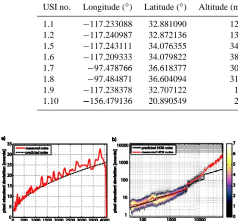
Fig. 10. Photon transfer curve for a USI system for (a) a 12-bit image, and (b) an 3
HDR image. The theoretical minimum shot noise limit is shown as a black line, and 4
the median of the noise distribution at each count value is shown in red. In (b), the 5
density of the pixel standard deviation distribution is shown behind the curves. 6
7
Figure 10. Photon transfer curve for a USI system for (a) a
12-bit image, and (b) an HDR image. The theoretical minimum shot noise limit is shown as a black line, and the median of the noise distribution at each count value is shown in red. In (b), the density of the pixel standard deviation distribution is shown behind the curves.
tion is approximately normal by the central limit theorem, and thus the rms noise (which is the same as the standard de-viation of the noise since the mean is zero) from each frame can be summed in quadrature to obtain the rms shot noise cij,shotin an HDR exposure, i.e.,
cij,shot=g
v u u t
P X
k tref
tk
e2ij,shot
k, (8)
wherek is the individual frame index,P is the number of frames, which ranges from one to three in this work. The ac-tual rms noise present in an HDR image was computed using the method described for Fig. 10a, and is shown in Fig. 10b. The noise is compared to the shot noise limit (Eq. 7, black line, Fig. 10b), where the number of frames in the HDR com-position is determined using the algorithm described in the previous section. The use of different combinations of frames can be seen as sharp jumps in the theoretical minimum in Fig. 10b.
The curves presented in Fig. 10 are similar to photon trans-fer curves (PTCs) which characterize not only shot noise, but all random noise present in the image sensor. Noise sources such as dark current and read noise are subtracted out of a PTC. The closeness of the curves to the shot noise limit indi-cates that for the USI system, sources of noise other than shot noise are small in both the 12-bit image, and the HDR com-position. The fluctuations in each curve, and the dips below
the theoretical minimum occur because a limited number of samples were taken (10 frames). Above 15 000 counts, very few samples were present in the HDR images, so noise in this region is not well characterized here.
4.7 Stray light
The red-blue-ratio image (RBR), defined as the ratio of the red channel to the blue channel, is the most common feature used for cloud detection. Clear sky has a relatively low RBR and clouds have a higher RBR. RBRs typically span between 0.4 and 1.2 for the USI, and the threshold for cloud is about 0.5. Stray light, due to exposure of the optical assembly to the direct beam, results in spots and artifacts in the image that are brighter and more spectrally neutral than they should be, resulting in either false positive cloud detections when the stray light pushes a hazy sky above the cloud threshold, or missing clouds due to contamination of the clear sky library (see Chow et al., 2011, or Yang et al., 2014, for details).
In order to characterize the stray light present in our sys-tem, we used a simple, hand-held shade to block the sunlight. The shade used was not much larger than the dome and was held at a considerable distance so as to sufficiently shade the entire optical assembly while minimizing the number of pix-els occupied by the shade within the image. Measurements were conducted on a clear day (13 May 2013) and shaded and un-shaded images were taken 30 s apart. By comparing images captured with and without the shading device, we can observe the effect of stray light on the resulting images. Three different pairs of images are compared in Fig. 11. First, a normal image is compared to one taken with the dome re-moved. Second, with the dome removed, images taken with and without the shade are compared. The third and final comparison considers shaded and un-shaded images with the dome on. The latter comparison gives the best estimate of the total effect of stray light on the images produced by the USI, while the first two allow us to qualitatively separate ef-fects due to the dome and the lens. To quantify the efef-fects of stray light, the residual fractional intensity(I2−I1) /I1is
computed and shown in the left column of Fig. 11, whereI1
is the image with the shade (or without dome, pair a), andI2
47 1
2
Fig. 11. Stray light from the dome (top), lens and neutral density filter (middle), and
3
whole system (bottom). The left column shows the fractional change in intensity due 4
to stray light, while the right column shows the shift in the red-blue ratio from the 5
shaded to unshaded image. Images were recorded against a clear (blue) sky, so 6
stray light shifts toward the red. Note the scale change between (a) and (b),(c) in the 7
left column. 8
Figure 11. Stray light from the dome (top), lens and neutral density
filter (middle), and whole system (bottom). The left column shows the fractional change in intensity due to stray light, while the right column shows the shift in the red-blue ratio from the shaded to un-shaded image. Images were recorded against a clear (blue) sky, so stray light shifts toward the red. Note the scale change between (a) and (b, c) in the left column.
The following stray light effects were identified: (1) an overall increase in measured intensity averaging 12 % across the image (Fig. 11c-i); (2) concentric ring-like reflections off the front face of the camera lens that reflect off the inner-surface of the dome (Fig. 11a vs. b); (3) particularly strong (and bluish) forward scattering off the dome (bright circle in Fig. 11a-ii); (4) sharp reflections off of elements in the opti-cal assembly, visible as spots along the intersection of the so-lar principal plane and the image plane (all); (5) a “swoopy” shape resulting from reflection of sunlight off the rear gelatin neutral density (ND) filter at the back of the lens (all); and (6) vertical smear that results near the sun from signal over-flow during sensor readout (all); (7) at higher solar eleva-tions (Fig. 12), a reflection of the sun off the surface of the image sensor. Here, the solar principal plane is defined by camera optical axis and the vector to the sun. The dome de-creases the average image intensity by about 46 % because of the ND acrylic used (Fig. 11a vs. b and c). While the dome surface was clean during testing, in normal operations dirt
Figure 12. Stray light comparison between two designs of the USI; (a) design with filter, and (b) design with modified aperture.
or scratches on the dome will result in additional scattering with a specific pattern that changes not just with the position of the sun, but also as a function of time since last cleaning.
Stray light impacts of the modified aperture (Sect. 2.1) versus the ND filter were qualitatively evaluated by visu-ally inspecting clear sky images such as those in Fig. 12. The following differences between the modified aperture and the wide-open, filtered configuration are noted: (i) reflec-tion from the ND filter surface is, naturally, missing in the model without a filter; (ii) the 9250 µm aperture in the fil-tered configuration exhibits a pair of reflections of the sun striking the image sensor that become visible at high solar elevations (when the direct-beam is nearly orthogonal to the image plane); this has not been observed using the modified aperture; (iii) the modified aperture shows a larger number of circles along the diameter containing the sun (i.e., intersec-tion of the solar principal plane and the image plane); (iv) a “feathery” radial pattern is sometimes observed near the sun with the modified aperture, arising from imperfections in the circularity of the aperture; (v) the modified aperture has a more prominent smear stripe because the selected aperture diameter allows more light into the camera; and (vi) pro-totypes with extremely small apertures exhibited diffraction rings around the sun (Fig. 3). Effect (iii) occurred because the antireflective black-oxide coating applied to the steel was mistakenly polished by the machinist, which increased its re-flectivity.
(concen-tric circles) and the region 90◦from the sun along the solar principal plane being the most prominent features. The clear sky library (CSL, Chow et al., 2011) is built from un-shaded images with the dome on (e.g., the RBR images used to con-struct Fig. 11c-ii), and stray light features are included in the cloud detection thresholds. Many of the stray light features are captured well by the CSL because they are functions of both solar zenith and sun-pixel angle. This becomes prob-lematic when the sun is shaded by clouds because the fea-tures are not present. This leads to significant problems de-tecting cloud near the sun, because as clouds pass and inter-mittently shade the sun, the RBR of clear sky and the clouds fluctuates, and a single threshold becomes problematic (Yang et al., 2014).
To reduce the impact of stray light, we have performed ex-perimentation with a stray light ratio lookup table as a func-tion of solar zenith angle, sun-pixel angle, and image zenith angle (similar to the clear sky library, Chow et al., 2011). However, the results, while promising, were inconsistent and thus are not reported here. A more robust approach based on generating synthetic, stray-light-free images with a 3-D ra-diative transfer model is currently being investigated. From our experience using the USI for forecasting, the stray light features discussed here negatively affect image quality and result in identifiable forecast performance degradation. Yang et al. (2014) have implemented adjustments to the cloud de-tection methods of Chow et al. (2011) to specifically address solar power forecast errors due to stray light. In future work we hope to develop corrections for the USI imagery so that stray light levels in imagery are reduced prior to being input into the cloud detection algorithms.
4.8 Color balancing
The neutral density filters currently used in the USI (Kodak Wratten 2, no. 96 ND3.0) introduce a color cast to the image. Basic color correction is performed by selecting a region of cloud that should be a neutral grey color and scaling the red, green, and blue signals relative to each other such that neu-tral grey is achieved. This color correction has been applied to many of the images shown above, and is useful when con-verting RGB images to other color spaces such as HSV, but has little effect on the red-blue-ratio. In the future we may use a color reference chart (e.g., the IT8.7/2-1993 calibration target) in order to improve the color balance of USI images in a way that might impact forecasting performance more.
5 Deployment experience
The UCSD USI system has been deployed across the United States (Table 3). The predominant cloud types in coastal California (USIs 1.1, 1.2, 1.9) are marine stratocumulus. In Kahului, Hawaii there are persistent orographic clouds over the West Maui Mountains to the west-northwest of USI 1.10
which makes it an interesting place to study non-advective solar forecast schemes. Redlands, California is hot and dry, and usually clear, but often sees higher ice clouds and larger synoptic systems. In Billings, Oklahoma there is a wide di-versity of cloud conditions that occur from high ice clouds, to lower cumulus clouds. Solar forecasting algorithms may have location dependent performance, and testing compo-nents of an algorithm in multiple locations can help to iden-tify shortcomings and areas for improvement.
The data gathered from the two instruments in Billings, Oklahoma are of particular interest because they were fielded at a United States Department of Energy Atmospheric Radi-ation Measurement Program field site (the Southern Great Plains site). The site includes a diverse suite of measure-ment equipmeasure-ment, including cloud radar covering a number of bands, several lidar systems, shortwave and longwave ra-diometers, aerosol measurements, and a Doppler wind pro-filer. These collocated measurements will be used to assess the performance of a number of remote sensing algorithms developed for the USI.
6 Conclusions and future work
Clouds have a high degree of spatial complexity and the in-tensity range within a single scene can be over five orders of magnitude (including the sun). For solar forecasting applica-tions, it is important to capture this information at a high spa-tial and radiometric resolution to facilitate the development of advanced algorithms and techniques. The UCSD Sky Im-ager system is a step in this direction. Ten instruments have been built and can be made available to other researchers. The units come with a camera and system control software and an extensive library of processing tools is available. The developers are also open to commercializing the instrument and extensive design documentation is available.
Acknowledgements. This work would not have been possible
without extensive student support in the design, fabrication, and assembly of the USI. We would like to thank, in no particular order, Caspar Hanselaar, Edmundo Godinez, William Gui, Fe-lipe Mejia, Prithvi Sundar, Dan Erez, Scott Kato, Amy Chiang, Jessica Traynor, Kristen Ostosh, Tyler Capps, Sebastian Schwarz-fischer, Sebastian Pangratz, Christian Faltermeier, Nick Truong, Salil Kektar, Jeff Yeh, Max Twogood, Alex Turchik, Danielle Don-nely, Emily Davis, and last, but not least the Victors Fung (1) and Piovano (2). We also appreciate funding from the Panasonic Corporation, the Department of Energy High Solar PV Penetration Award Number EE-0004680, and the California Energy Commis-sion contract 500-10-060.
References
Anderson, M.: Studies of the woodland climate: I. The photo-graphic computation of light conditions, J. Ecol., 52, 27–41, doi:10.2307/2257780, 1964.
Bayer, B. E.: Color Filter Array, U.S. Patent No. 3,971,065, U.S. Patent and Trademark Office, Washington, DC, 1975.
Brown, H. E.: The canopy camera, Station Paper 72, Fort Collins, CO: U.S. Department of Agriculture, Forest Service, Rocky Mountain Forest and Range Experiment Station, 1962.
Cazorla, A., Olmo, F. J., and Alados-Arboledas, L.: Development of a sky imager for cloud cover assessment, J. Opt. Soc. Am., 25, 29–39, doi:10.1364/JOSAA.25.000029, 2008.
Chow, C. W., Urquhart, B., Lave, M., Dominguez, A., Kleissl, J., Shields, J. E., and Washom, B.: Intra-hour forecasting with a total sky imager at the UC San Diego solar energy testbed, J. Sol. En-erg., 85, 2881–2893, doi:10.1016/j.solener.2011.08.025, 2011. Debevec, P. and Malik, J.: Recovering high dynamic range
radi-ance maps from photographs, Proceedings of the ACM SIG-GRAPH’97, Los Angeles CA, 369–378, 1997.
Dupree, W., Morse, D., Chan, M., Tao, X., Iskenderian, H., Reiche, C., Wolfson, M., Pinto, J., Williams, J. K., Albo, D., Dettling, S., Steiner, M., Benjamin, S., and Weygandt, S.: The 2008 CoSPA forecast demonstration (collaborative storm prediction for avia-tion), Proceedings of the 89th Meeting of the American Meteo-rological Society, Special Symposium on Weather – Air Traffic, Phoenix, AZ, 2009.
Dye, D.: Looking skyward to study ecosystem dynamics, Eos T. Am. Geophys. Un., 93, 141–143 doi:10.1029/2012EO140002, 2012.
Faugueras, O: Three-dimensional Computer Vision, MIT Press, Cambridge, ISBN 0-262-06158-9, 1993.
Feister, U. Shields, J. E.: Cloud and radiance measurements with the VIS/NIR Daylight Whole Sky Imager at Lindenberg (Germany), Meteorol. Z., 14, 627–639, doi:10.1127/0941-2948/2005/0066, 2005.
Fu, C. L. and Cheng, H. Y.: Predicting solar irradiance with all-sky image features via regression, J. Sol. Energ., 97, 537–550, doi:10.1016/j.solener.2013.09.016, 2013.
Gohari, S. M. I., Urquhart, B., Yang, H., Kurtz, B., Nguyen, D., Chow C. W., Ghonima, M., and Kleissl, J.: Comparison of solar power output forecasting performance of the Total Sky Imager and the University of California, San Diego Sky Imager, Energy Procedia, 49, 2340–2350, doi:10.1016/j.egypro.2014.03.248, 2014.
Gonzales, Y., Lopez, C., and Cuevas, E.: Automatic observation of cloudiness: analysis of all-sky images, TECO-2012, WMO Technical Conference on Meteorological and Environmental In-struments and Methods of Observation, Brussels, Belgium, 16– 18 October 2012.
Hartley, R. and Zisserman, A.: Multiple view geometry in computer vision, Cambridge University Press, ISBN: 9780511811685, doi:10.1017/CBO9780511811685, 2004.
Hill, R.: A lens for whole sky photographs, Q. J. Roy. Meteorol. Soc., 50, 227–235, doi:10.1002/qj.49705021110, 1924. Huo, J. and Lu, D.: Comparison of cloud cover from all-sky imager
and meteorological observer, J. Atmos. Ocean. Tech., 29, 1093– 1101, doi:10.1175/JTECH-D-11-00006.1, 2012.
Johnson, R. W., Koehler, T. L., and Shields, J. E.: A Multi-Station Set of Whole Sky Imagers and A Preliminary Assessment of the
Emerging Data Base, Proceedings of the Cloud Impacts on DOD Operations and Systems – 1988 Workshop, 159–162, 1988. Johnson, R. W., Hering, W. S., and Shields, J. E.: Automated
Vis-ibility and Cloud Cover Measurements with a Solid-State Imag-ing System, University of California, San Diego, Scripps Institu-tion of Oceanography, Marine Physical Laboratory, SIO Ref. 89-7, GL- TR-89-0061, NTIS No. ADA216906, 1989.
Kalisch, J. and Macke, A.: Estimation of the total cloud cover with high temporal resolution and parametrization of short-term fluc-tuations of sea surface insolation, Meteorol. Z., 17, 603–611, doi:10.1127/0941-2948/2008/0321, 2008.
Klebe, D. I., Blatherwick, R. D., and Morris, V. R.: Ground-based all-sky mid-infrared and visible imagery for purposes of char-acterizing cloud properties, Atmos. Meas. Tech., 7, 637–645, doi:10.5194/amt-7-637-2014, 2014.
Long, C. N. and DeLuisi, J. J.: Development of an automated hemi-spheric sky imager for cloud fraction retrievals, Proceedings of the 10th Symposium on Meteorological Observations and Instru-mentation, Phoenix, Arizona, American Meteorological Society, 171–174, 1998.
Long, C. N., Sabburg, J. M., Calbó, J., and Pagès, D.: Re-trieving cloud characteristics from ground-based daytime color all-sky images, J. Atmos. Ocean. Technol., 23, 633–652, doi:10.1175/JTECH1875.1, 2006.
Mann, S. and Picard, R. W.: On being “undigital” with digital cam-eras: extending dynamic range by combining differently exposed pictures, Technical Report 323, MIT Media Lab Perceptual Com-puting Section, 1994 (also in: Proceedings of Imaging Science and Technology 48th annual conference, 422–428, 1995). Marquez, R. and Coimbra, C. F. M.: Intra-hour DNI forecasting
methodology based on cloud tracking image analysis, J. Sol. En-erg., 91, 327–336, doi:10.1016/j.solener.2012.09.018, 2013. Mathiesen, P. and Kleissl, J.: Evaluation of numerical
weather prediction for intra-day solar forecasting in the continental United States, J. Sol. Energ., 85, 967–977, doi:10.1016/j.solener.2011.02.013, 2011.
Mathiesen, P., Collier, C., and Kleissl, J.: A high-resolution cloud-assimilating numerical weather prediction model for solar irradiance forecasting, J. Sol. Energ., 92, 47–61, doi:10.1016/j.solener.2013.02.018, 2013.
Miyamoto, K.: Fish Eye Lens, J. Opt. Soc. Am., 54, 1060–1061, doi:10.1364/JOSA.54.001060, 1964.
Nakajima, T., Tonna, G., Rao, R., Boi, P., Kaufman, Y., and Holben, B.: Use of sky brightness measurements from ground for remote sensing of particulate polydispersions, J. Appl. Optics, 35, 2672– 2686, doi:10.1364/AO.35.002672, 1996.
Perez, R., Cebecauer, T., and Šúri, M.: Semi-empirical satellite models, chapter 2 in: Solar Energy Forecasting and Resource Assessment, edited by: Kleissl, J., Elsevier, ISBN: 978-0-12-397177-7, 2013.
Reda, I. and Andreas, A.: Solar position algorithm for so-lar radiation applications, J. Sol. Energ., 76, 577–589, doi:10.1016/j.solener.2003.12.003, 2004.
camera for obtaining sky radiance at three wavelengths, At-mos. Meas. Tech., 5, 2013–2024, doi:10.5194/amt-5-2013-2012, 2012.
Sebag, J., Krabbendam, V. L., Claver, C. F., Andrew, J., Barr, J. D., and Klebe, D.: LSST IR camera for cloud monitoring and observation planning, Proceedings of the International Society of Photonics and Optics, Ground-based and Airborne Telescopes II conference (SPIE 7012), 7012, doi:10.1117/12.789570, 2008. Shields, J. E., Johnson, R. W., and Karr, M. E.: Automated Whole Sky Imagers for Continuous Day and Night Cloud Field Assess-ment, Proceedings of the Cloud Impacts on DOD Operations and Systems Conference, 1993a.
Shields, J. E., Johnson, R. W., and Koehler, T. L.: Automated Whole Sky Imaging Systems for Cloud Field Assessment, Proceedings of the Fourth Symposium on Global Change Studies, American Meteorological Society, Boston, 17–22 January, 1993b. Shields, J. E., Johnson, R. W., Karr, M. E., and Wertz, J. L.:
Auto-matic day/night whole sky imager for field assessment of cloud cover distributions and radiance distributions, Proceedings of the 10th Symposium on Meteorological Observations and In-strumentations, Phoenix, AZ, American Meteorological Society, Boston, 165–170, 1998a.
Shields, J. E., Karr, M. E., Tooman, T. P., Sowle, D. H., and Moore, S. T.: The Whole Sky Imager – A Year of Progress, Proceedings of Eighth Atmospheric Radiation Measurement (ARM)Science Team Meeting, 1998b.
Shields, J. E., Karr, M. E., Johnson, R. W., and Burden, A. R.: Day/night whole sky imagers for 24-h cloud and sky assess-ment: history and overview, J. Appl. Optics, 52, 1605–1616, doi:10.1364/AO.52.001605, 2013.
Stumpfel, J., Tchou, C., Jones, A., Hawkins, T., Wenger, A., and De-bevec, P.: Direct HDR capture of the sun and sky, AFRIGRAPH 2004, 3rd International Conference on Computer Graphics, Vir-tual Reality, Visualization and Interaction in Africa, Cape Town, South Africa – 3–5 November, doi:10.1145/1029949.1029977, 2004.
Urquhart, B., Ghonima, M., Nguyen, D., Kurtz, B., Chow, C. W., and Kleissl, J.: Sky imaging systems for short-term solar fore-casting, chapter 9 in: Solar Energy Forecasting and Resource Assessment, edited by: Kleissl, J., Elsevier, ISBN: 978-0-12-397177-7, 2013.
Urquhart, B., Kurtz, B., and Kleissl, J.: Sky camera geometric cali-bration using solar observations, submitted, 2015.
Wood-Bradley, P., Zapata, J., and Pye, J.: Cloud tracking with opti-cal flow for short-term solar forecasting, Proceedings of the 50th Conference of the Australian Solar Energy Society, Melbourne, December 2012.