Interactions between a Treatment and
Scalar/Functional Predictors
Hyung G. Park
Submitted in partial fulfillment of the requirements for the degree
of Doctor of Philosophy under the Executive Committee of the Graduate School of Arts and Sciences
COLUMBIA UNIVERSITY
2018Hyung G. Park All Rights Reserved
Flexible Regression Models for Estimating
Interactions between a Treatment and
Scalar/Functional Predictors
Hyung G. Park
In this dissertation, we develop regression models for estimating interactions between a treatment variable and a set of baseline predictors in their effect on the outcome in a randomized trial, without restriction to a linear relationship. The proposed semiparamet-ric/nonparametic regression approaches for representing interactions generalize the notion of an interaction between a categorical treatment variable and a set of predictors on the outcome, from a linear model context.
In Chapter 2, we develop a model for determining a composite predictor from a set of baseline predictors that can have a nonlinear interaction with the treatment indicator, implying that the treatment efficacies can vary across values of such a predictor without a linearity restriction. We introduce a parsimonious generalization of the single-index models that targets the effect of the interaction between the treatment conditions and the vector of predictors on the outcome. A common approach to interrogate such treatment-by-predictor interaction is to fit a regression curve as a function of the predictors separately for each treatment group. For parsimony and insight, we propose a single-index model with multiple-links that estimates a single linear combination of the predictors (i.e., a single-index), with treatment-specific nonparametrically-defined link functions. The approach emphasizes a focus on the treatment-by-predictors interaction effects on the treatment outcome that are relevant for making optimal treatment decisions. Asymptotic results for estimator are obtained under possible model misspecification. A treatment decision rule based on the derived single-index is defined, and it is compared to other methods for estimating optimal treatment decision rules. An application to a clinical trial for the treatment of depression
unspecified main effect of the predictors on the outcome. This extension greatly increases the utility of the proposed regression approach for estimating the treatment-by-predictors interactions. By obviating the need to model the main effect, the proposed method extends the modified covariate approach of [Tian et al., 2014] into a semiparametric regression framework. Also, the approach extends [Tianet al., 2014] into generalK treatment arms.
In Chapter 4, we introduce a regularization method to deal with the potential high dimensionality of the predictor space and to simultaneously select relevant treatment effect modifiers exhibiting possibly nonlinear associations with the outcome. We present a set of extensive simulations to illustrate the performance of the treatment decision rules estimated from the proposed method. An application to a clinical trial for the treatment of depression is presented to illustrate the proposed approach for deriving treatment decision rules.
In Chapter 5, we develop a novel additive regression model for estimating interactions be-tween a treatment and a potentially large number of functional/scalar predictor. If the main effect of baseline predictors is misspecified or high-dimensional (or, infinite dimensional), any standard nonparametric or semiparametric approach for estimating the treatment-by-predictors interactions tends to be not satisfactory because it is prone to (possibly severe) inconsistency and poor approximation to the true treatment-by-predictors interaction ef-fect. To deal with this problem, we impose a constraint on the model space, giving the orthogonality between the main and the interaction effects. This modeling method is par-ticularly appealing in the functional regression context, since a functional predictor, due to its infinite dimensional nature, must go through some sort of dimension reduction, which essentially involves a main effect model misspecification. The main effect and the interac-tion effect can be estimated separately due to the orthogonality between the two effects, which side-steps the issue of misspecification of the main effect. The proposed approach extends the modified covariate approach of [Tian et al., 2014] into an additive regression model framework. We impose a concave penalty in estimation, and the method simulta-neously selects functional/scalar treatment effect modifiers that exhibit possibly nonlinear interaction effects with the treatment indicator. The dissertation concludes in Chapter 6.
List of Figures v
List of Tables xi
1 Introduction 1
2 A Single-index model with multiple-links 6
2.1 Introduction . . . 6
2.2 A Single-index model with multiple-links (SIMML) . . . 7
2.3 Criteria for estimation . . . 9
2.3.1 Profile likelihood maximization . . . 9
2.3.2 MaximizingL2 distance between two link functions . . . . 10
2.4 Estimation . . . 11
2.5 Asymptotic theory . . . 13
2.6 Simulation studies . . . 14
2.6.1 Precision of estimators . . . 14
2.6.2 ITR performance . . . 17
2.6.3 Coverage probability of asymptotic 95% confidence intervals . . . 20
2.7 Application to data from a randomized clinical trial . . . 21
2.8 Discussion . . . 28
3 A Constrained single-index model with multiple-links for interactions 29 3.1 Introduction . . . 29
3.2 Models . . . 31
3.4.1 Algorithm . . . 33
3.4.2 Main effect augmentation . . . 35
3.4.3 Details for estimating the projection vector . . . 35
3.5 Connection to the modified covariate approach . . . 36
3.5.1 Sufficient reduction . . . 36
3.5.2 Linear GEM models . . . 37
3.5.3 K≥3 case . . . 39
3.5.4 Extension to a semiparametric model . . . 39
3.5.5 Some geometric intuition . . . 41
3.6 Simulation examples . . . 43
3.6.1 Estimation criterion illustration . . . 43
3.6.2 ITR performance forK= 2 case . . . 46
3.6.3 ITR performance forK= 3 case . . . 50
3.7 Discussion . . . 52
4 A Sparse constrained single-index model with multiple-links 53 4.1 Introduction . . . 53
4.2 Treatment effect modifier selection . . . 54
4.2.1 A constrainedL1 regularization . . . . 55
4.2.2 Algorithm for treatment effect modifier selection . . . 56
4.3 Simulation examples . . . 58
4.3.1 ITR performance forK= 2 case . . . 58
4.3.2 ITR performance forK= 3 case . . . 61
4.3.3 Treatment effect modifier selection performance . . . 62
4.4 Application: Depression RCT . . . 63
4.5 Discussion/Extension to a partially linear single-index model (PLSIM) with multiple-links . . . 68
5.2 Method . . . 71
5.2.1 Functional additive model with multiple-links (FAMML) . . . 71
5.2.2 Criterion . . . 74
5.2.3 Estimation . . . 76
5.3 Simulation illustration . . . 80
5.3.1 Treatment effect modifier selection performance . . . 80
5.3.2 ITR performance . . . 82
5.4 Application . . . 87
5.5 Discussion . . . 93
6 Conclusion 94 Bibliography 94 A Appendix for Chapter 2 102 A.1 Assumptions for Theorem 1 and Theorem 2 . . . 102
A.2 The asymptotic covariance matrix in Theorem 2 . . . 103
A.3 Proof . . . 103
A.3.1 Proof of Theorem 1 . . . 103
A.3.2 Proof of Theorem 2 . . . 104
A.4 Table for Section 2.6.3 Coverage probability of asymptotic 95% confidence intervals . . . 108
B Appendix for Chapter 3 110 B.1 A justification for the equivalence between MCA and SIMML under a linear link restriction . . . 110 B.2 Proof . . . 111 B.2.1 Proof of Theorem 3 . . . 111 B.2.2 Proof of Lemma 1 . . . 112 B.2.3 Proof of Lemma 2 . . . 112 iii
C.2 Some computational notes 1 . . . 115 C.3 Some computational notes 2 . . . 117
D Appendix for Chapter 5 119
D.1 Proof . . . 119 D.1.1 Proof of Theorem 4 . . . 119
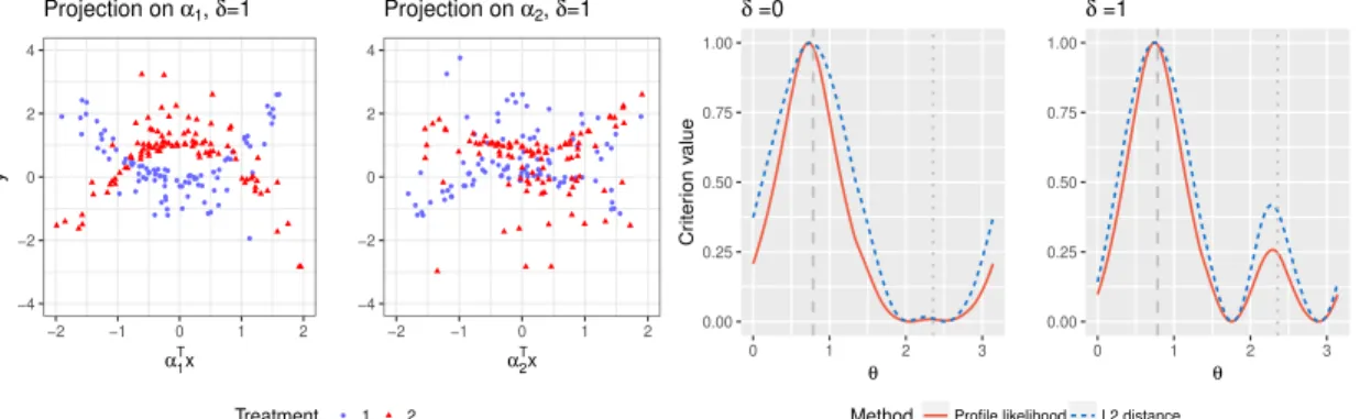
2.1 The first two panels: the outcomes simulated under model (2.18) whenδ= 1, plotted against the “first” index α>1X in the first panel, and against the “second” indexα>2Xin the second panel, for the two treatment groups (blue dots and red triangles respectively). The third (δ = 0 case) and the fourth (δ= 1 case) panels: the criterion functions of the profile likelihood maximizer (the red solid curve) and theL2 distance maximizer (the blue dotted curve), averaged over 100 simulated datasets, each scaled to have height 1. The dashed grey vertical line indicates the angle θ1 = π/4 that corresponds to
α1, and the vertical dotted grey line indicatesθ2= 3π/4 that corresponds to
α2. . . 16 2.2 The first panel shows the linear contrastCt’s (ω = 0), the second panel the
moderately nonlinear contrast Ct’s (ω = 0.5), and the third panel displays
highly nonlinear contrastCt’s (ω = 1). Data points are generated from model
(2.19) withδ = 0 andp= 5. The fourth and the fifth panel shows thelinear
(ν= 0) and thenonlinear main effectM (ν = 1), respectively. . . 18 2.3 Boxplots of the PCDs of the treatment decision rules obtained from 200
training datasets for each of the four methods. Each panel corresponds to one of the six combinations ofω∈ {0,0.5,1}andν ∈ {0,1}: the shape of the contrast functionsCt’s controlled byω; the shape of the main effect function M controlled by ν; the number of predictors p ∈ {5,10}. The sample sizes are n1 = 40, n2 = 30. . . 19
data points; the placebo group is the blue solid curve and the active drug group is the red dotted curve. The associated 95% confidence bands of the regression curves were also plotted. . . 23 2.5 Pair of estimated link functions (g1 and g2) obtained from SIMML with the
“main effect adjusted” profile likelihood (first panel), SIMML with the (main effect un-adjusted) profile likelihood (second panel), and the linear GEM model estimated under the criterion maximizing the difference in the linear regression slopes (third panel), respectively, for the placebo group (blue solid curves) and the active drug group (red dotted curves). The 95% confidence bands were constructed conditioning on the single-index coefficient α. For each group, observed values of the outcomes are plotted against the estimated index. . . 24 2.6 Top row: Violin plots of the estimated values of ITRs based on each of the
individual predictors x1, . . . , x9, determined from univariate nonparametric and linear regressions, respectively, obtained from 500 randomly split testing sets (with higher values preferred). Bottom row: The estimated single-index coefficients α1, . . . , α9, associated with the covariates x1, . . . , x9. The associ-ated 95% confidence intervals obtained from BCa bootstrap with 500 repli-cations are illustrated. Estimated significant coefficients are marked with ∗
on the top. . . 25 2.7 Boxplots of the estimated values of ITRs obtained from the 500 randomly
split testing sets (higher values are preferred). The estimated values (and the standard deviations) are given as follows: SIMML*: 9.34 (2.68); SIMML: 8.72 (2.68); K-Index: 8.04 (2.69); K-LR: 8.36 (2.69); linGEM: 8.22 (2.67); All PBO: 6.17 (2.63); All DRG: 7.57 (2.67). . . 27
the fitted ˆY for the model E(Y T) is the orthogonal projection of the observed Y onto the plane of the column space spanned by the intercept and the treatments. The fitted vector for the intercept-only model E(Y |1) is ¯Y1n. In the picture, the magnitude of the “effect” of the intercept (i.e., averaging), which gets modified by the treatment (i.e., treatment-specific averaging), can be quantified by the squared length of ˆY −Y¯1n. . . 41 3.2 The empirical mean squared error criterion of the constrained SIMML, the
na¨ıve SIMML, and the MCA, respectively, averaged over 200 simulated datasets, for simulation set A. The vectorαcorresponds to the angleθ1 =π/4, and the “nuisance” vector µ corresponds to the angle θ2 = 3π/4. The grey dashed vertical line indicates the angle θ1, corresponding toα, and the grey dotted vertical line indicates θ2, corresponding to µ. . . 45 3.3 The empirical mean squared error criterion of the constrained SIMML, the
na¨ıve SIMML, and the MCA, respectively, averaged over 200 simulated datasets, for simulation set B. The vectorαcorresponds to the angleθ1 =π/4, and the “nuisance” vector µ corresponds to the angle θ2 = 3π/4. The grey dashed vertical line indicates the angleθ1, corresponding toα, and the grey vertical dotted line indicatesθ2, corresponding toµ. . . 45 3.4 Top panels: boxplots of the PCDs of the ITRs estimated from the four
meth-ods (SIMML, MCA, K.AM, and K.LR) for the nonlinear contrast case. Lower panels: boxplots of the PCDs of the ITRs for the linear contrast case. For each case,n∈ {200,400}and p∈ {5,10} were considered. . . 48 3.5 Upper panel: illustration of gt(ν), t ∈ {1,2,3}, with simulated data points
underδ = 0. Lower panels: boxplots of the PCDs of the ITRs estimated from the four different methods (SIMML, L.GEM, L.AM, and K.LR) applied to 200 simulated datasets, for each combination of n∈ {200,400}, p ∈ {5,10}
and δ∈ {1,3}. . . 51
panels: boxplots of the PCDs of the ITRs for the linear contrast case. For each case,n∈ {200,400},p∈ {100,200}, and δ∈ {1,2} were considered. . 60 4.2 Boxplots of the PCDs of the ITRs estimated from the four methods (SIMML,
L.GEM, K.AM, and K.LR), for each combination of n ∈ {200,400}, p ∈ {100,200}, and δ∈ {1,3}, obtained from 200 simulated runs. . . 62 4.3 Observed values of the response variable against the estimated single-index
(= α>X) from the SIMML in the top panel, and against individual pre-dictors, “Flanker Accuracy”, “(Age) x (Flanker Accuracy)”, and “(Age) x (Baseline HRSD)”, from left to right, respectively, in the bottom panels. Pairs of estimated treatment-specific B-spline approximated link functions with the associated 95% confidence bands were overlaid; in the top panel, the confidence bands were constructed conditioning onα. . . 66 4.4 Boxplots of the values (2.22) of the ITRs estimated from the six different
approaches, obtained from the 500 randomly split testing sets. Higher values are preferred. . . 68 5.1 Figure describes a set of orthogonal coordinate axes. g∗j,T(u) corresponds
to the axis for the T-by-u interaction effect. Its orthogonal complement, gj,T∗ (u)⊥, corresponds to the axis for the main effect of u. The interaction effect is quantified by βj. Here, u=hαj,xji, to be optimized over αj. The regression plane is represented by the two orthogonal axes. The nonlinearity is captured by gj,T∗ (hαj,xji), and the scale is captured by βj. . . 74 5.2 The average number of treatment effect modifiers “correctly selected” (in the
panels with gray background), and “incorrectly selected” (in the panels with white background), respectively, as the training sample sizenvaries from 50 to 500, for eachp∈ {50,100}. Two methods were compared: 1) the proposed semiparametric FAMML, and 2) a FAMML with the links gj,T restricted to be linear (Linear-FAMML). . . 82
respectively. . . 84 5.4 Boxplots of the PCDs of the ITRs for the simulation set “A”, obtained from
100 replications, estimated from the following three methods: (1) FAMML: the proposed semi-parametric method satisfying the orthogonality constraint (5.6); (2) F-MCA: the modified covariate approach with efficiency augmen-tation; (3) Separate FLR: two separate FLR models estimated separately for each of the two treatment groups. For each case, n ∈ {100,200,400} and δ ∈ {0,1,2} were considered. . . 86 5.5 Boxplots of the PCDs of the ITRs for the simulation set “B”, obtained from
100 replications, estimated from the following three methods: (1) FAMML: the proposed semi-parametric method satisfying the orthogonality constraint (5.6); (2) F-MCA: the modified covariate approach with efficiency augmen-tation; (3) Separate FLR: two separate FLR models estimated separately for each of the two treatment groups. For each case, n ∈ {100,200,400} and δ ∈ {0,1,2} were considered. . . 87 5.6 The locations for the 19 electrode channels. “A1” and “A2” were not used.
Those marked in red circles are the selected electrodes from the fitted FAMML (5.5): “FP1”, “C3”, “O1”, “O2”, and “PZ”. . . 89 5.7 Top panels: observed CSD curves from the 5 channels, FP1, C3, O1, O2,
and PZ, for the active drug group (red dashed curves) and for the placebo group (blue dotted curves), over a frequency range of 3 to 16 Hz, when the participants’ eyes are closed. Bottom panels: estimated projection functions (αj’s) for the selected 5 functional predictors (from left to right: FP1, C3, O1, O2, and PZ). . . 90
j 1,4,6,12,15 , corresponding to the channels, FP1, C3, O1, O2, and PZ. Overlaid are the estimated treatment-specific link functions (gj,1, gj,2) for the placebo group in the dotted blue, and the active drug group in the dotted red curves; the associated 95% confidence bands were constructed conditioning on the projection functions, αj’s. . . 91 5.9 The scatter plots of thekth partial residual vs. thekth scalar predictors,k∈
{1,3,4}, the baseline HRSD, age, and the baseline HRSD-by-age interaction, respectively, where all variables are centered at 0. The variable “sex” (z2) was not selected by the model. Overlaid are the estimated treatment-specific functions (hk,1, hk,2) for the placebo group in the solid blue, and the active drug group in the dotted red curves; the associated 95% confidence bands of the regression curves were plotted. . . 91 5.10 Boxplots of the values of the ITRs, obtained from 300 randomly split testing
sets, estimated from the four approaches: FAMML, Linear-FAMML, giving everyone the placebo, and giving everyone the active drug. Higher values are preferred. . . 92
2.1 Description of the p= 9 baseline covariates (means and SDs); the estimated values (“Indiv. Value”) of treatment decision rules from each individual co-variate, using either the B-spline regression (“nonpar.”) or the linear regres-sion (“linear”); the estimated singe-index of the three (single-index based) methods, with the estimated values of the treatment decision rules. . . 22 4.1 Comparison of the treatment effect modifier selection performance of the
SIMML and the MCA. The averaged number of correctly (C.) selected treat-ment effect modifiers and incorrectly (I.C.) selected treattreat-ment effect mod-ifiers, averaged out of 200 simulation runs, are reported. Superior perfor-mances are indicated in bold-faced. . . 63 4.2 Description of p = 22 baseline predictors and the estimated L1
regular-ized/unregularized index coefficients α from the SIMML and the MCA, re-spectively. All coefficient estimates were scaled to have unitL2 norm. . . . 65 A.1 The proportion of time (“Coverage”) that the asymptotic 95% confidence
interval contains the true value of αj, j ∈ {1, . . . ,5}, for contrast functions with a single crossing (ω= 0), and contrasts functions with multiple crossings (ω= 1), with varyingn(=n1+n2, where 2n1= 3n2) . . . 109
First, I would like to give my sincere thanks to my adviser, Dr. Todd Ogden, for his guidance, encouragement, and assistance. Looking back upon my time at Columbia, I feel so fortunate to have known and worked with him as his student. Not only he taught me valuable statistical insights but also he served as a role model who I hope to emulate.
I would also like to deeply thank the chair of my dissertation committee, Dr. Ian McKeague, for his advice and encouragement. I would also like to give my sincere thanks to the other members of my committee: Dr. Eva Petkova, Dr. Min Qian, and Dr. Seonjoo Lee, for their time and insightful comments.
I am thankful to my fellow doctoral students who took the classes together and the professors who taught me. I gratefully acknowledge the fellowship I received from the department. I would also like to thank Dr. Eva Petkova and Dr. Thad Tarpey for their guidance and invaluable support on our projects together, and thank Dr. Seonjoo Lee for the opportunity to serve as a research assistant and the project with her. I give my sincere thanks to Dr. Nan Laird, Dr. L.J. Wei, Dr. Francesca Dominici, and Dr. Armin Schwartzman, for their encouragements when applying to my doctoral study. I give my special thanks to Dr. Gail Gong, who first taught me how to do research work. I also express my thanks to Dr. Mingue Park and Dr. Hyungjun Cho, for their invaluable supports.
My deepest thanks go to my mother and grandmother. Thank you for your unwavering belief in me and for all the love and the goodness that I received from you, everywhere in my life.
Just as a tree takes the sunlight to synthesize organic molecules, I feel that I live my life out of the love and the support from the people surrounding me.
Chapter 1
Introduction
Precision medicine represents a powerful and effective general approach for disease treat-ment and prevention that takes into account individual variability in genetic structure, environment, and lifestyle for each person. Its growth is not only helped by technological advances in detecting and measuring a wide range of biomedical information, such as brain imaging (structure, function, connectivity), molecular, genomic, cellular, clinical, behav-ioral, physiological, and environmental characteristics, but also helped by the increasing pace of developing treatment options. The most daunting challenge for precision medicine is discovery of the treatment implications of the available complex and large-scale biological information.
To develop strategies for precision medicine, it is important to identify treatment and predictor interactions ([Royston and Sauerbrei, 2008], [Tian et al., 2014]) particularly in the setting of randomized clinical trials (RCT). There are many RCTs dedicated to dis-covering the treatment implications based on individual patient’s characteristics. Just in major depressive disorder (MDD), for example, recent large-scale studies include iSPOT-D: International Study to Predict Optimized Treatment for Depression, PReDICT: Predictors of Remission in Depression to Individual and Combined Treatments, and EMBARC: Estab-lishing Moderators and Biosignatures of Antidepressant Response for clinical Care, among others.
Recent breakthroughs in biotechnology allows a vast amount of data available for explor-ing for potential interaction effect with the treatment and assistexplor-ing in the optimal treatment
decision for individual patients ([Tianet al., 2014]). For example, data from modern med-ical experiments include more and more commonly not only traditional clinmed-ical measures, but also increasingly complex information such as genetic information (e.g., [van’t Veer and Bernards, 2008]) and brain structure or functions, measured from neuroimaging modalities such as magnetic resonance imaging (MRI), functional MRI (fMRI), electroencephalogram (EEG), among others. This motivates the need for developing an efficient and also flexible statistical method for discovery of biomarkers from high-dimensional data, specifically de-signed to estimate the interactions between a treatment and high-dimensional pretreatment predictors.
In particular, development of individualized treatment decisions rules (ITRs) based on patient characteristic data measured at baseline is an increasingly important topic in pre-cision medicine. Much research has been done since the seminal papers of [Murphy, 2003] and [Robins, 2004]. Regression-based methodologies are intended to optimize the ITRs by estimating treatment-specific mean responses (e.g., [Qian and Murphy, 2011], [Zhanget al., 2012], [Gunteret al., 2011], [Lu et al., 2011], among others), while seeking robustness with respect to model misspecification. Extensions that allow functional data objects to be incorporated as baseline predictors have also been developed (e.g., [McKeague and Qian, 2014], [Ciarleglioet al., 2015a]). Machine learning approaches for developing ITRs originate from computer science literature, and can often be framed in the context of classification problems ([Zhang et al., 2012], [Zhang et al., 2012]), for example, the outcome weighted learning (OWL) (e.g., [Zhao et al., 2012], [Zhao et al., 2015], [Song et al., 2015]) based on support vector machines, tree-based classification (e.g. [Laber and Zhao, 2015]), and the [Kanget al., 2014] method based on adaptive boosting, among others. In these settings of optimizing ITRs, a major challenge is in the discovery of biomarkers that exhibit interac-tion effects with the treatment indicator when large amount of patient characteristics are available.
Suppose we are given pre-treatment predictors X ∈ X, a treatment variable T that takes a value in a finite, discrete treatment space, say, T ={1,· · · , K}, and a real-valued response variable Y. We assume that a larger Y is preferred, without loss of generality. Let the distribution of (Y, T, X) be denoted by P. An ITR D:X → T is a deterministic
decision rule that mapsX into the treatment spaceT. For any fixed ITRD, letPD denote the distribution of (Y, T, X) conditioning on T = D(X), i.e., the treatments are chosen according to the rule D. Let ED denote the expectation with respect to PD. A natural measure for the effectiveness of D is the expected outcome that would have resulted if D
had been used to choose treatment for the entire study population
V(D) =ED(Y), (1.1)
which is often called the “value” associated with D ([Murphy, 2005], [Qian and Murphy, 2011]). A larger value of (1.1) is preferred. Therefore, an ITR that maximizes the function
D →V(D) over all Dis called optimal. It can be easily verified that any D0(X) with
D0(X) ∈ arg max t∈T E
(Y |X, T =t), X ∈ X (1.2) is optimal ([Murphy, 2005], [McKeague and Qian, 2014]), where E denotes expectation underP.
A first natural approach to estimate the optimal ITR is then to maximize an empirical version of the mean response (1.1) (or its surrogate) over a class of ITRs, in a classifi-cation context, for example, as in OWL ([Zhao et al., 2012]). Although the classification approaches can be appealing in many settings, in this dissertation, we will focus on a regres-sion approach that estimates the conditional expectations E(Y |X, T =t), t∈ T in (1.2), as the regression-based approaches are most frequently utilized in practice, and often come with great interpretability. We will employ a two-step procedure (e.g., [Qian and Murphy, 2011]) that first estimates the conditional expectationE(Y |X, T) using a regression model and then from this estimated conditional expectation derives the estimated treatment.
In (1.2), if the conditional expectation is modeled correctly, then the two-step proce-dure consistently estimates the optimal ITR. [Qian and Murphy, 2011] derived several finite sample upper bounds on the difference between the mean response (1.1) to the optimal ITR and the mean response to the estimated ITR. If the part of the model for the conditional expectation involving the treatment-by-predictors interaction effect is correct, then the up-per bounds imply that, although a surrogate two-step procedure is used, the estimated ITR is consistent. The upper bound of [Qian and Murphy, 2011] is an improvement over that of ([Murphy, 2005]), in the sense that the upper bound depends only on how well we
approximate the interaction effect term, and not on the main effect term of the conditional expectation. These upper bounds guarantee that if the T-by-X interaction effect is consis-tently estimated (for example, estimated under the squared error loss), then the value (1.1) of the estimated ITR will converge to the optimal value.
However, if the approximation space for the interaction effect does not provide an inter-action effect term close to the true interinter-action effect term of the conditional expectation, then the two-step procedure does not provide the best value of the considered ITRs in the approximation space ([Qian and Murphy, 2011]). This is due to the “mismatch” ([Murphy, 2005]) between the loss functions (weighted 0-1 loss for directly maximizing the value and the squared error loss for approximating the conditional expectation). In other words, if the interaction effect model is misspecified, then the ITR obtained from the two-step procedure may not be the best ITR within the class of ITRs defined by the model. [McKeague and Qian, 2014] noted that this issue also arises when a smooth surrogate of the empirical value function is maximized ([Zhao et al., 2012]).
The primary focus of this dissertation is on developing flexible regression approaches to accurately approximate the interaction effect term of the conditional expectation. The semiparametric/nonparametric regression approaches that we develop in this dissertation for estimating the interaction effect term will reduce the concerns regarding the mismatch between the two loss functions, that occur from the misspecification of the interaction effect term in the model.
[Qian and Murphy, 2011] approximated the conditional expectation usingL1 penalized least squares with a rich linear model. However, the approach is generally not robust to the main effect model misspecification, and is restricted to a parametric regression model. The presence of main effect, which often have much bigger effect on the outcome than the treatment interactions, makes the consistent estimation of the interaction effect very difficult, if the main effect model is misspecified or is high-dimensional. [Tian et al., 2014] proposed a novel approach to consistently estimate the covariates and treatment interactions without the need for modeling main effects. Their method modified the covariates in a simple way, and then fit a standard model using the modified covariates and no main effects. However, the approach is limited to a linear regression framework. In realistic situations,
the knowledge of the true functional forms for models of interactions is often lacking, and a linear model is generally restrictive.
The main contribution of this dissertation is in generalizing the work of [Tian et al., 2014] to a single-index model framework in Chapter 3, and to an additive model framework in Chapter 5. These extensions provide robust and flexible regression approach to devel-oping ITRs in many situations, particularly when we deal with a large number of baseline predictors, that includes multiple functional predictors.
The thesis is organized as follows. In Chapter 2, we introduce a flexible model for determining composite predictors that permit nonlinear association with the outcome. In Chapter 3, we will consider a more general model where we assume an unspecified structure for the main effect component. In Chapter 4, we use aL1 regularization to consider a large model for the treatment effect modification. In Chapter 5, we develop a sparse additive regression model for estimating interactions between a treatment and a large number of functional/scalar predictors. The thesis concludes in Chapter 6.
Chapter 2
A Single-index model with
multiple-links
2.1
Introduction
In precision medicine, a critical concern is to identify baseline measures that have distinct relationships with the outcome from different treatments so that patient-specific treatment decisions can be made ([Murphy, 2003], [Robins, 2004]). Such variables are called treatment effect modifiers, and these can be useful in determining a treatment decision rule that will select a treatment for a patient based on observations made at baseline. There is a growing need to extract treatment effect modifiers from (usually noisy) baseline patient data that, more and more commonly, consist of a large number of clinical and biological characteristics. Typically, treatment effect modifiers (or, “moderators”) are identified either one by one, using one model for each potential predictor, or from a large model which includes all potential predictors and their (two-way) interactions with treatment, and then testing for significance of the interaction terms, almost exclusively using linear models. In the linear model context, [Petkovaet al., 2016] proposed a model using a linear combination (i.e., an index) of patients’ characteristics, termed a generated effect modifier (GEM) constructed to optimize the interaction with a treatment indicator. Such a composite variable approach is especially appealing for complex diseases such as psychiatric diseases, in which each baseline characteristic may only have a small treatment modifying effect. In such settings,
it is uncommon to find variables that are individually strong moderators of treatment effects. Here we present novel flexible methods for determining composite variables that permit non-linear association with the outcome. In particular, the proposed methods allow the conditional expectation of the outcomes to have a flexible treatment-specific link function with an index. We define the index to be a one-dimensional linear combination of the co-variates. This approach is related to single-index models ([Brillinger, 1982], [Stoker, 1986], [Powellet al., 1989], [Hardleet al., 1993], [Xia and Li, 1999], [Horowitz, 2009], [Antoniadis
et al., 2004]), as well as to single-index model generalizations such as projection pursuit
regression ([Friedman and Stuetzle, 1981]) and multiple-index models ([Xia, 2008], [Yuan, 2011]). We employ a single projection of the covariates (i.e., an index) to summarize the variability of the baseline covariates, and multiple link functions to connect the derived single-index to the treatment-specific mean responses; we call these single-index models with multiple-links (SIMML) models. This single-index models with multiple-links pro-vides a parsimonious generalization of the single-index model in modeling the effect of the interaction between a categorical treatment variable and a vector-valued covariate. The dependence of treatment-specific outcomes on a common single index improves the inter-pretability, and helps determining ITRs. This approach extends the notion of a “treatment effect modifier” from the linear model setting, to a single-index model framework, to define a nonparametric generated effect modifier.
2.2
A Single-index model with multiple-links (SIMML)
Let X = (x1, . . . , xp)> ∈ Rp denote the set of covariates. Let T denote the categorical (treatment assignment) variable of interest, taking values in {1, . . . , K} with probabilities (π1, . . . πK) that sum to one. LetY ∈R denote an outcome variable, where a higher value of Y is preferred. We focus on data arising from a randomized experiment, however, the method can be extended to observational studies.
A conventional approach to study the effect of the interaction between Xand the treat-ment indicator T on an outcome is to fit a regression model separately for each of the K treatment groups, as functions of X. For instance, a single-index model can be fitted
sep-arately for each treatment group t, resulting inK indices, β>t X,t∈ {1, . . . , K}. We refer to this as a K-index model; it has the form
E(Y |T =t, X =x) =gt(βt>x) (t= 1, . . . , K), (2.1) where both the treatment-specific nonparametric link functions gt(·), and the treatment-specific index vectors βt ∈ Rp, need to be estimated for each group t. [Wu and Rolling, 2016] proposed this model for dimension reduction in optimizing ITRs. (The vectors βt need to satisfy some identifiability condition ([Lin and Kulasekera, 2007]).) While this is a reasonable approach, the K indices of model (2.1) lack useful interpretation as effect modifiers and often lead to over-parametrization.
The SIMML constrains the βt in (2.1) to be equal, and it requires separate nonpara-metrically defiend curves for each treatmenttas a function of a single indexα>X common for all t:
E(Y |T =t, X=x) =gt(α>x) (t= 1, . . . , K), (2.2) where both the linksgt and the vectorα need to be estimated. Due to the nonparametric nature of gt, the scale of α is not identifiable in (2.2) and to address this we restrict α to be in Θ ={α= (α1, . . . , αp)>|Pjp=1α2j = 1, αp >0}, i.e., to be in the upper hemisphere of the unit sphere.
If the true model for the treatment-specific outcomeYtis not a SIMML, then the SIMML can be regarded as theL2projection of the treatment specific mean outcomemt(X) =E(Yt| X) on the single indexu=α>X,
gt(u) =E(mt(X)|α>X =u) (t= 1, . . . , K), (2.3) for each given α. Specifically, suppose the true treatment-specific model can be expressed as
Yt=mt(X) +σt(X) (t= 1, . . . , K), (2.4) in which E(|X) = 0, E(2 |X) = 1. Let R(α) =PKt=1πtE Yt−gt(α>X)
2
, where gt is defined in (2.3) and let
α0 := arg min α∈Θ
Then α0 can be shown to be the minimizer of the cross-entropy (e.g., [Mackay, 2003]) between the SIMML (2.2) and the general model (2.4) under the Gaussian noise assumption. Here, the cross-entropy of an arbitrary distribution with the probability density (or, mass) f, with respect to another reference distribution P is defined as EP(−logf), where the expectation is take with respect to the distribution P. Model (2.3) evaluated at α0 can be viewed as the “projection” (in the sense of the closest point) of the true distributionP
(2.4) onto the space Θ of the SIMML distribution, using the Kullback-Leibler divergence as a distance measure.
The SIMML (2.2) allows a visualization useful for characterizing differential treatment effects, varying with the single indexα>X. As X∈Rp varies, the mean response of model (2.2) changes only in the specific directionα∈Θ, and the effect of varyingX, described by the link functionsgt, is different for each treatment conditiont∈ {1, . . . , K}. Therefore, the single index can be viewed as a useful biosignature that can describe differential treatment effects, provided thatgt6=gt0 for at least one pairt, t0∈ {1, . . . , K}.
2.3
Criteria for estimation
2.3.1 Profile likelihood maximization
While any nonparametric smoother can be employed to approximate the unspecified smooth link functionsgt(·) in (2.2), in this chapter, we will apply cubic splines. Specifically,gt(u)≈
η>t Z(u), for someηt∈Rd. Here,Z(u) =
h
B1(u), . . . , Bd(u)
i>
∈Rdconsists of a set ofd normalized cubicB-spline basis functions [de Boor, 2001]. For ease of notation, the number of basis functions,d, is taken to be the same across treatments but in practice dmay vary by treatment. Let nt be the sample size for the tth treatment group and n = PKt=1nt denote the total sample size. For a givenα, letZα,t denote the B-spline evaluation matrix (nt×d), so that the ith row is Z(α>Xti)>, which is the B-spline evaluation of the ith individual from thetth treatment group. The subscript αin the matrix Zα,t highlights its dependence onα.
For sample data, SIMML (2.2) can be represented by
h Y i n×1 = h Zα i n×Kd h η i Kd×1+ h i n×1, (2.6)
where Y =
Y1>, . . . ,YK>>
is the observed response vector in which Yt ∈ Rnt, Zα is n×Kdblock-diagonal B-spline design matrix of the Zα,t’s, η =
η1>, . . . ,η>K> is the B -spline coefficient vector, and=
>1, . . . ,>K>
is a mean zero noise vector with covariance matrixσ2In.
Givenα, we define then×nsingle index projection matrix to beSα=Zα ZTαZα
−1
ZTα. Assuming Gaussian noise and treating η as a nuisance parameter, the negative “profile” loglikelihood ofα, up to a constant multiplier, is
Q(α) =kY −SαYk2. (2.7) We define the profile likelihood estimator of the index parameterα as
ˆ
α = arg min α∈Θ
Q(α). (2.8)
Each link functions gt(·) in (2.2) can be estimated by ˆ
gt(u) =Z(u)> ZTαˆ,tZαˆ,t
−1
ZTαˆ,tYt (t= 1, . . . , K), (2.9) whereZαˆ,t is Zα,t evaluated atα= ˆα.
2.3.2 Maximizing L2 distance between two link functions
A natural criterion for choosingαin the SIMML (2.2) in terms of moderator analysis is to maximize an interaction effect. In the special case of linear link functions in the SIMML
gt(α>X) =γt0+γtα>X (t= 1, . . . , K). (2.10) [Petkovaet al., 2016] proposed estimating αto maximize the variability of the GEM slopes γt’s, weighted by their respective probabilitiesπt; this was called the “numerator” criterion because it corresponds to maximizing the numerator of aF-test statistic for significance of an interaction effect.
Analogously, for nonlineargt(·),αcan be chosen to maximize the variance of the distance between any two link functions, e.g., g1(·) and g2(·) of (2.2). Assuming that the outcome has been centered at 0 for each treatment group and that the observations are independent,
maximizing the variance corresponds to maximizing the L2 distance between the two link functions over α∈Θ, which simplifies to
EX g1(α>X)−g2(α>X) 2 = Z g21(α>x)fX(x)dx+ Z g22(α>x)fX(x)dx, (2.11) wherefX(·) is the density of X(assumed equal across treatment groups due to randomiza-tion). Givenα, define thent×ntmatrixSα,t=Zα,t Z>α,tZα,t
−1
Z>α,tfort= 1,2. Then the index coefficientsα can be chosen to maximize the corresponding empirical approximation of the L2 distance (2.11) W(α) =Y1TSα,1Y1/n1+Y2TSα,2Y2/n2, (2.12) and ˆ α= arg max α∈Θ W(α). (2.13)
The associated link functions ˆgt(·) can be obtained by (2.9).
2.4
Estimation
Suppose we have a set of observations{(Yti, Xti)in=1t }Kt=1. For each candidate α, [Wang and Yang, 2009] suggested to take an integral transformation of each candidate index variable
α>Xti,α∈Θ, touα,ti =Fp(α>Xti), whereFp is a re-scaled centered Beta{(p+ 1)/2,(p+ 1)/2} cumulative distribution function
Fp(ν) =
Z ν/R
−1
(1−t2)(p−1)/2Γ(p+ 1)/(Γ{(p+ 1)/2}22p)dt, ν ∈[−R, R],
in whichR= maxt,i|α>Xti|. For any fixedα, this (transformed) index has a quasi-uniform [0,1] distribution, and it is reasonable to use equally-spaced knots on [0,1] when applying spline smoothing ([Wang and Yang, 2009]).
In an attempt to avoid being trapped in local minima in solving (2.8), we employ a variant of a gradient descent algorithm; we adopt elements of the Cuckoo search ([Yang and Deb, 2009], [Yang and Deb, 2014]). The Cuckoo search considers multiple (say,C >1) evolving candidate solutions, where each of the C candidates takes independent random walks, specified by the step size, s > 0 which follows a heavy-tailed distribution (we take
the absolute value of the standard Cauchy distribution), with some direction inRp(we take the negative of the gradient of the criterion functionQ(α), which we denote by−∇∈Rp). From the rth candidate at the hth update, ˆα((rh)) ∈ Rp, a new position ˆα(h+1)
(r) ∈ R p is generated by
ˆ
α((hr)+1)= ˆα((hr))−s((hr))l((rh))∇((hr)), (2.14) where s((hr)) is the random step size; ∇((rh)) ∈ Rp is the gradient ∇ evaluated at α = ˆα(h)
(r); l((hr)) ∈Ris an adaptive multiplier which is [Ong, 2014]
l((rh))= lL+ (lU−lL)(Q((rh))−Q(minh))/(Q(avgh)−Q (h) min), if Q (h) (r) < Q (h) avg lU, if Q((hr))≥Q(avgh) , (2.15)
wherelL>0 andlU ≥lLare pre-specified minimum and maximum step sizes, respectively, depending on the scale of the problem. In (2.15), Q((hr)) corresponds to the criterion value (2.7); Q(minh) is the minimum, and Q(avgh) is the average of the criterion values at the hth
update, respectively, computed from C candidate solutions. Intuitively, when a candidate solution is close to the minimum, the algorithm focuses more on the local search. The jth component of the gradient ∇is
∇j(α) = 2Y>(In−Sα) ˙Z(αj)(Z>αZα)−1Z>αY, j∈ {1, . . . , p}, (2.16) where ˙Z(αj) is ann×dK block diagonal matrix with the blocks equal to
˙ Z(αj,t) = h B10(Fp(Xtα))∗F 0 p(Xtα)∗Xt,j . . . B 0 d(Fp(Xtα))∗F 0 p(Xtα)∗Xt,j i nt×d
for t = 1, . . . , K. Here, Xt is nt×p covariate matrix of the tth treatment group, the jth column Xt,j corresponds to the jth covariate from the tth treatment, and ∗ denotes element-wise multiplication.
To obtain the L2 distance maximizer of Section 2.3.2, instead of the profile likelihood maximizer, we simply change the objective function to be the negative of the criterion function of (2.12), and∇((hr)) to be the negative gradient of (2.12), evaluated at α= ˆα((hr)).
The algorithm reduces to an ordinary gradient descent, if s((hr)) in (2.14) is set to be non-random andC= 1. In such cases, we can take as an initial solution ˆα(h=1) of gradient descent the leading eigenvector of the weighted “between-group” covariance matrix of the
ordinary least-square regression coefficient vector (weighted by group assignment probabil-itiesπt), i.e., the solution that maximizes the variability of the GEM slopes from the linear model of [Petkovaet al., 2016].
Algorithm 1 An algorithm for estimating the single index coefficient α
1: CenterYtat0 and center and scale Xt for each t= 1, . . . , K.
2: Seth←1. GenerateC candidate solutions, A(h) =αˆ(1), . . . ,αˆ(C)
>
, where ˆα(r)∈Θ.
3: Evaluate (2.7) for each ˆα(r), and obtain Q(h)=
Q( ˆα(1)), . . . , Q( ˆα(C))
>
.
4: forh= 1,2, . . . until convergencedo
5: Set h←h+ 1.
6: Set A(h)←A(h−1), andQ(h)←Q(h−1).
7: Compute Q(avgh) andQ
(h)
min fromQ(h), obtain the multipliers
h
l((1)h), . . . , l((Ch))i >
in (2.15).
8: Compute theC×p gradient matrix
h
∇( ˆα((1)h)), . . . ,∇( ˆα((hC)))
i>
by using (2.16).
9: for r= 1, . . . , C do
10: Generate a new solutionα(tempr) ,(h) via (2.14) fromα((hr)). Setαtemp(r) ,(h) to be in Θ.
11: Evaluate (2.7) atαtemp(r) ,(h), and denote the evaluated value by Qtemp(r) ,(h).
12: if Qtemp(r) ,(h)< Q((rh)) thenα((hr))←αtemp(r) ,(h) andQ((hr))←Qtemp(r) ,(h).
13: end for
14: end for
15: Output ˆα that corresponds toQ(minh).
Once ˆα is obtained, the estimates of the link functions ˆgt(·) can be obtained by (2.9). The fitted SIMML is then ˆgt(Fp( ˆα>X)), t∈ {1, . . . , K}.
2.5
Asymptotic theory
In this section, we establish the asymptotic results of the profile estimator ˆα in (2.8), under possible misspecification, when the true model is assumed to be (2.4). We assume that the data consist ofnrandom vectors{(Yi, Ti, Xi), i= 1, . . . , n}on an underling probability space (Ω,F,P), in which{(Yi, Ti, Xi) :Ti =t}arentidentically distributed random vectors fort= 1, . . . , K, with the ratio nt/nconverging to a constant, πt∈(0,1) almost surely, as
n→ ∞. Observations between groups are assumed to be independent.
Let us denote the pth component of the vector α0 by α0,p(> 0, since α0 ∈ Θ). By the completeness property of R, we can always find some c > 0 such that α0,p ≥ c, and therefore, without loss of generality, we may assume thatα0 is in a compact set Θc={α= (α1, . . . , αp)>∈Rp|Ppj=1α2j = 1, αp ≥c}, with an appropriate choice of smallc >0. Theorem 1. (Consistency) Under Assumption 1 to 5 in the Appendix, αˆ → α0 almost
surely.
The proof of Theorem 1 is given in the Appendix. To avoid the complication from the restricted parameter space Θc, we will consider instead the “pth component removed” R(α) in (2.5) as follows R(α−p) =R α1, . . . , αp−1, q 1−(α21+· · ·+α2p−1), (2.17) where a vector α−p = (α1, α2, . . . , αp−1) ∈ Rp−1 lives inside the unit ball. Let the “pth component removed” value of the optimal α0 be denoted by α0,−p ∈ Rp−1. Similarly, let the corresponding profile estimator ˆα in (2.8) be denoted by ˆα−p∈Rp−1.
Theorem 2. (Asymptotic Normality) Under Assumption 1 to 5 in the Appendix,√n( ˆα−p−
α0,−p)→ N(0,Σα0,−p) in distribution, with asymptotic covariance matrix
Σα0,−p =H
−1
α0,−pWα0,−pH
−1
α0,−p, where the matrixHα0,−p is the Hessian matrix H(α−p) =
∂2
∂α−p∂αT−p
R(α−p) evaluated at α−p =α0,−p, and the matrix Wα0,−p is defined in the
Ap-pendix.
The proof ofTheorem2 is given in the Appendix. The asymptotic confidence intervals for the index coefficients can be constructed using the asymptotic covariance inTheorem2.
2.6
Simulation studies
2.6.1 Precision of estimators
We investigate the precision of the α estimators in the simple case of K = 2 treatment groups and p = 2 baseline covariates. The covariates X = (x1, x2)> are generated from
N(0,ΨX), where ΨX = 1 0.1 0.1 1
. The outcomes in the two treatment groups are
simu-lated underYt=mk(X;δ) +t withk∼ N(0,0.12)(t= 1,2), where m1(X;δ) = 0.5(α>1X)2−δ/3(α>2X)2 m2(X;δ) = 1−0.5(α>1X)2+δ/3(α>2X)2, (2.18) in which α1 = (1,1)>/ √ 2 and α2 = (−1,1)>/ √
2. If δ = 0, the data generation model (2.18) is a “genuine” SIMML (2.2), and the single index of the SIMML is α>1X. However, if δ 6= 0, model (2.18) is not in the class of SIMML since it involves two indices, α>1X and α>2X, and the approximate SIMML is gt(α>X) = E[mt(X;δ) | α>X], t = 1,2, for some α ∈Θ. The parameter δ in (2.18) controls the relative influence of α1 and α2. We consider two cases in the simulations: δ = 0 (“genuine” SIMML) andδ = 1, for which α1 has a stronger influence than α2 (and so α>1X can be considered as the more important composite covariate that modifies the effect of treatments).
We investigate how the estimator of the index coefficient α = (a1, a2)> of (approx-imated) SIMML (2.2) obtained via maximizing the SIMML profile likelihood (i.e., ˆα in (2.8)) compares to the estimator obtained by maximizing theL2 distance between the two link functions from (2.13). For the purposes of visualization we expressα∈Θ⊂R2in polar coordinates. If Cartesian coordinates are transformed into polar coordinates, (a1, a2)> on the unit half circle Θ can be represented by a single parameter,θ for 0≤θ < π, where θis an angle in radians. Then α1 corresponds to θ1 = π/4 andα2 corresponds to θ2 = 3π/4. As a function of the angleθ, the criterion function of an unbiased estimator would have a peak atθ1 and a smaller one at θ2.
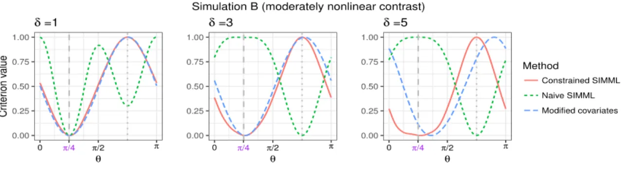
We simulated 100 data sets under the above described setup (2.18), and averaged the values of the criterion functions (the profile likelihood and the L2 distance, respectively) for each θ ∈[0, π]. The resulting averaged criterion functions are shown on the third and the fourth panels of Figure 2.2, for the case of δ = 0 and δ = 1, respectively. Both the profile likelihood andL2 distance maximizers have a global peak atθ1 =π/4 and a smaller local peak at θ2 = 3π/4. The profile likelihood maximizer, however, shows a sharper peak around the true valueθ1compared to theL2distance maximizer, indicating better efficiency in estimation, for bothδ ∈ {0,1}.
−4 −2 0 2 4 −2 −1 0 1 2 α 1 T x y Projection on α1, δ=1 −4 −2 0 2 4 −2 −1 0 1 2 α 2 T x Projection on α2, δ=1 Treatment 1 2 0.00 0.25 0.50 0.75 1.00 0 1 2 3 θ Cr iter ion v alue δ =0 0.00 0.25 0.50 0.75 1.00 0 1 2 3 θ δ =1
Method Profile likelihood L2 distance
Figure 2.1: The first two panels: the outcomes simulated under model (2.18) when δ= 1, plotted against the “first” index α>1X in the first panel, and against the “second” index
α>2X in the second panel, for the two treatment groups (blue dots and red triangles respec-tively). The third (δ = 0 case) and the fourth (δ = 1 case) panels: the criterion functions of the profile likelihood maximizer (the red solid curve) and the L2 distance maximizer (the blue dotted curve), averaged over 100 simulated datasets, each scaled to have height 1. The dashed grey vertical line indicates the angle θ1 =π/4 that corresponds to α1, and the vertical dotted grey line indicatesθ2 = 3π/4 that corresponds to α2.
2.6.2 ITR performance
A treatment decision function,D(X) :Rp 7→ {1, . . . , K}, mapping a subject’s baseline char-acteristics X∈Rp to one of K available treatments, defines an ITR for the single decision time point ([Murphy, 2003], [Robins, 2004], [Cai et al., 2011], [Qian and Murphy, 2011]). Given covariatesX, an ITR based on SIMML isD(X) = arg maxt∈{1,...,K} gt(α>X).We in-vestigate the performance of the estimated ITRs of the formD(X) = arg maxt∈{1,...,K} E[Y | X, T =t],where the conditional expectation is obtained from various modeling procedures. The baseline covariate vector X = (x1, . . . , xp)> ∼ N(0,ΨX), with ΨX having 10s on the diagonal and 0.1 everywhere else. We consider K= 2 with different noise levels for the two treatment groups: 1 ∼ N(0,0.42), 2 ∼ N(0,0.22) . The outcome data are generated under the following fairly broad model
Yt=δM(µ>X;ν) +Ct(α>X;ω) +t (t= 1,2). (2.19) As a function of the indexµ>X, M is referred to as the “main effect” ofX. As functions of the other indexα>X, theCt’s are referred to as the “contrast” functions that define the treatment-by-Xinteraction. Here, we will use the parametersν andω to control the degree of non-linearity of M and Ct’s, respectively.
An optimal treatment decision rule depends only on the Ct’s, not on M or the t’s. The parameter δ in (2.19) controls the relative contribution of the Ct0s to the variance in the outcomes, and is calibrated to obtain the relative contribution of 0.35. The contrast functions Ct’s in (2.19) are set to
Ct(u;ω) =
C
1(u;ω) = +1−cos 0.5πωu
+ 0.5(u−ω) C2(u;ω) =−1 + cos 0.5πωu−0.5(u−ω),
(2.20) where, if ω = 0, then the Ct’s are linear functions; and they are more nonlinear for larger values ofω. We considered three cases, corresponding tolinear (ω= 0),moderately nonlin-ear (ω= 0.5), and highly nonlinear (ω = 1)Ct’s, respectively, illustrated in the first three panels of Figure 2.2. We set the main effect functionM in (2.19) to be
M(u;ν) = 0.5u−sin(0.5πνu),
where, asν increases, the degree of nonlinearity in M increases. We considered two cases, ν = 0, corresponding to alinear M; andν= 1, corresponding to anonlinear M, illustrated
−1 0 1 2 −1 0 1 αTx y Linear Ck’s (ω=0) −1 0 1 2 −1 0 1 αTx Moder. nonlinear Ck’s (ω=0.5) −1 0 1 2 −1 0 1 αTx Highly nonlinear Ck’s (ω=1) Treatment 1 2 −1.0 −0.5 0.0 0.5 1.0 −2 −1 0 1 2 µTx y Linear M (ν=0) −1.0 −0.5 0.0 0.5 1.0 −2 −1 0 1 2 µTx Nonlinear M (ν=1)
Figure 2.2: The first panel shows the linear contrast Ct’s (ω = 0), the second panel the
moderately nonlinear contrastCt’s (ω= 0.5), and the third panel displayshighly nonlinear
contrastCt’s (ω= 1). Data points are generated from model (2.19) with δ= 0 and p= 5. The fourth and the fifth panel shows the linear (ν = 0) and the nonlinear main effect M (ν = 1), respectively.
in the fourth and the fifth panels of Figure 2.2. We considered p = 5 and p = 10 with
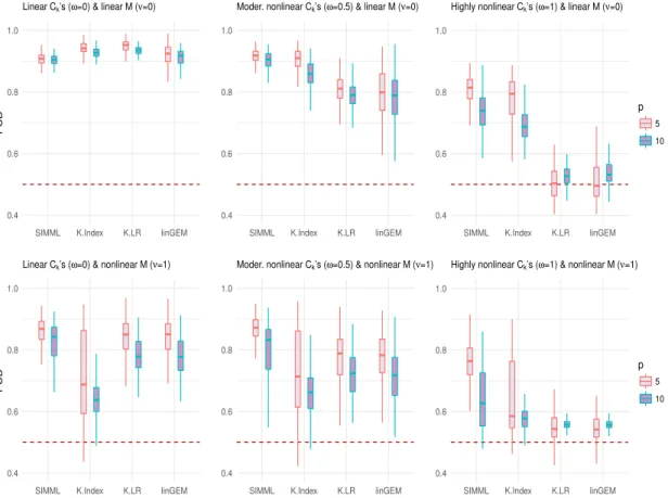
α = (1, . . . ,5)> and α = (1, . . . ,10)>, respectively, each standardized to have norm one. We set µ to be proportional to a vector of 1’s, standardized to have norm one. Two treatment groups were considered with unequal sample sizes: n1 = 40 and n2 = 30. We usedd= 5 B-spline basis functions. We compared the treatment decision rules determined based on the following regression models: (i) SIMML (2.2) estimated from maximizing the profile likelihood; (ii) theK-Index model (2.1) fitted separately for each treatment group by theB-spline approach of [Wang and Yang, 2009], denoted asK-Index; (iii) the linear GEM model ([Petkova et al., 2016]) estimated under the criterion of maximizing the difference in the treatment-specific slope, denoted as linGEM; and (iv) linear regression models fitted separately for each treatment group under the least squares criterion, denoted as K-LR. For each scenario, using the outcomeY from a simulated test set (of size 105), we computed the proportion of correct decisions (PCD) of the treatment decision rules estimated from each method. We reported the boxplots of PCDs obtained from 200 training datasets.
Figure 2.3 shows that SIMML outperformed all other methods, except for the case under the linear M and Ct’s in which all 4 approaches performed well. The K-Index method was clearly second best, under the linear M (ν = 0) (the top panels) with the nonlinear Ct’s (ω = 0.5 andω = 1). However, for more complex M function (ν = 1) (the bottom panels), the performance of the K-index model was considerably worse compared
0.4 0.6 0.8 1.0
SIMML K.Index K.LR linGEM
PCD
Linear Ck’s (ω=0) & linear M (ν=0)
0.4 0.6 0.8 1.0
SIMML K.Index K.LR linGEM
Moder. nonlinear Ck’s (ω=0.5) & linear M (ν=0)
0.4 0.6 0.8 1.0
SIMML K.Index K.LR linGEM
Highly nonlinear Ck’s (ω=1) & linear M (ν=0)
p 5 10 0.4 0.6 0.8 1.0
SIMML K.Index K.LR linGEM
PCD
Linear Ck’s (ω=0) & nonlinear M (ν=1)
0.4 0.6 0.8 1.0
SIMML K.Index K.LR linGEM
Moder. nonlinear Ck’s (ω=0.5) & nonlinear M (ν=1)
0.4 0.6 0.8 1.0
SIMML K.Index K.LR linGEM
Highly nonlinear Ck’s (ω=1) & nonlinear M (ν=1)
p 5 10
Figure 2.3: Boxplots of the PCDs of the treatment decision rules obtained from 200 training datasets for each of the four methods. Each panel corresponds to one of the six combinations of ω ∈ {0,0.5,1} and ν ∈ {0,1}: the shape of the contrast functions Ct’s controlled by ω; the shape of the main effect function M controlled by ν; the number of predictors p∈ {5,10}. The sample sizes are n1= 40, n2= 30.
to SIMML. When the underlying model is complex, given a relatively small sample size, the SIMML in which the treatment contrast was emphasized through the common single-index was more effective in estimating treatment decision rules than the K-Index model. As would be expected, additional complexity inCt’s (ω = 0.5 and ω = 1) had a greater effect on the performance of the more restrictive models (linGEM andK-LR) than it did on the flexible models (SIMML and K-index). It was clear that the number of covariates p also had a major impact on the performance of all methods. As p changed from 5 (red) to 10 (blue), the deterioration in performance was more pronounced for the K-Index model that requires separate fits for each treatment and thus involve estimation of more parameters (K(p−1) +Kd), than the more parsimonious SIMML with a fewer number of parameters (p−1 +Kd) to be estimated.
2.6.3 Coverage probability of asymptotic 95% confidence intervals
We present a simulation experiment that assesses the coverage probability of the asymptotic confidence intervals derived fromTheorem2. The data were generated under model (2.19) withδ = 0 (i.e., no main effect M) withp= 5 predictors. We set the SIMML index vector
α(= α0) to be stepwise increasing: (1, . . . ,5)>, normalized to have unit L2 norm. The associated contrast functions, Ct’s, are given by (2.20), and two levels of the curvature of the contrasts are considered, corresponding to a single and multiple-crossings cases, ω∈ {0,1}, respectively (see Figure 2.2). To set signal to noise ratio at 1 for both scenarios, the noise standard deviations were set to 0.64 and 0.89, corresponding toω = 0 andω = 1 respectively. We considered unequal sample sizes for theK= 2 groups by settingn=n1+n2 where 2n1 = 3n2. With varying n ∈ {100,200,400,800,1600,3200,6400}, the number of interior knots used in the B-spline approximation, was determined to be N =
h
n11/5.5
i
as recommended by [Wang and Yang, 2009]. Five hundred data sets were generated for all combinations of n and ω. For each (i.e., the jth) component αj of α, the proportion of times the 95% asymptotic confidence interval contains the true value of αj was recorded in the table in the Appendix. The 5th (i.e., the pth) element is estimated to satisfy the constraint α∈Θ in Theorem 2.
“nominal” coverage probability, with better coverage results for the single-crossing scenario (ω = 0) compared to the multiple-crossing scenario (ω= 1).
2.7
Application to data from a randomized clinical trial
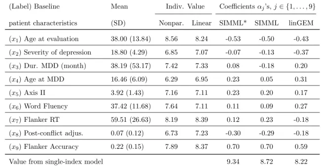
Major depressive disorder afflicts millions and, according to the World Health Organization, it is the leading cause of disability worldwide. It is a highly heterogeneous disorder, however, no individual biological or clinical marker has demonstrated sufficient ability to match individuals to efficacious treatment. Here we illustrate the utility of the proposed SIMML method for determining ITRs with an application to data from a randomized clinical trial comparing an antidepressant and placebo for treating depression.Of the 166 subjects, 88 were randomized to placebo and 78 to the antidepressant. In addition to standard clinical assessments, patients underwent neuropsychiatric testing prior to treatments. Patients were tested Flanker [Flanker and Eriksen, 1974] and A not B Working Memory (AnotB; [Herrera-Guzman et al., 2009]), for which reaction time (RT) and accuracy were assessed. In addition, RT was recorded for a choice task [Deary et al., 2011]. Four baseline clinical and demographic characteristics were also assessed: (i) current patient age; (ii) severity of depressive symptoms measured by the Hamilton Rating Scale for Depression (HRSD); (iii) duration of the current major depressive episode; and (iv) age of onset of first major depressive episode. Table 2.1 summarizes the information on thep= 9 baseline patient characteristics, X = (x1, . . . , x9)>, starting with the means and standard deviations of the original (untransformed) covariates. The treatment outcome Y was the improvement in symptom severity from baseline to week 8 and thus larger values of the outcome were better.
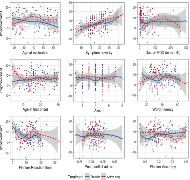
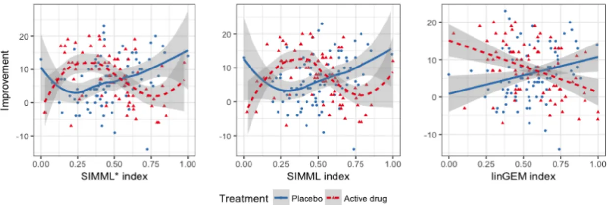
Figure 2.4 shows the outcome Y against each of the 9 baseline covariates for placebo (blue) and active drug (red). The estimated B-spline approximated curves are shown with the associated 95% confidence bands: the solid blue curves for the placebo group and the dotted red curves for the active drug group. From the figure, we can see that each individual covariate marginally has at most a small modifying treatment effect.
(Label) Baseline Mean Indiv. Value Coefficientsαj’s,j∈ {1, . . . ,9}
patient characteristics (SD) Nonpar. Linear SIMML* SIMML linGEM
(x1) Age at evaluation 38.00 (13.84) 8.56 8.24 -0.53 -0.50 -0.43 (x2) Severity of depression 18.80 (4.29) 6.85 7.07 -0.07 -0.13 -0.37 (x3) Dur. MDD (month) 38.19 (53.17) 7.42 7.33 0.08 -0.18 0.20 (x4) Age at MDD 16.46 (6.09) 6.29 6.95 0.23 0.05 0.31 (x5) Axis II 3.92 (1.43) 7.16 7.11 0.23 0.20 0.17 (x6) Word Fluency 37.42 (11.68) 7.64 7.11 0.11 0.09 0.27 (x7) Flanker RT 59.51 (26.63) 8.19 8.39 0.12 0.23 -0.18 (x8) Post-conflict adjus. 0.07 (0.12) 6.73 7.23 -0.30 -0.29 -0.18 (x9) Flanker Accuracy 0.22 (0.15) 7.89 8.37 0.70 0.70 0.59
Value from single-index model 9.34 8.72 8.22
Table 2.1: Description of the p = 9 baseline covariates (means and SDs); the estimated values (“Indiv. Value”) of treatment decision rules from each individual covariate, using either the B-spline regression (“nonpar.”) or the linear regression (“linear”); the estimated singe-index of the three (single-index based) methods, with the estimated values of the treatment decision rules.
Figure 2.4: For each of the 9 baseline covariates individually, treatment-specific spline approximated regression curves with 5 basis functions are overlaid on to the data points; the placebo group is the blue solid curve and the active drug group is the red dotted curve. The associated 95% confidence bands of the regression curves were also plotted.
Figure 2.5: Pair of estimated link functions (g1 and g2) obtained from SIMML with the “main effect adjusted” profile likelihood (first panel), SIMML with the (main effect un-adjusted) profile likelihood (second panel), and the linear GEM model estimated under the criterion maximizing the difference in the linear regression slopes (third panel), respectively, for the placebo group (blue solid curves) and the active drug group (red dotted curves). The 95% confidence bands were constructed conditioning on the single-index coefficientα. For each group, observed values of the outcomes are plotted against the estimated index. if everyone in the population receives treatment according to that rule, the “value” (V) (1.1) of a decision ruleD ([Qian and Murphy, 2011]):
V(D) =EX
EY|X[Y |X, T =D(X)]
. (2.21)
In Table 2.1, “Indiv. Value” refers to the estimated value of an ITR based on each individual covariate, based on two approaches for determining ITRs: the aforementioned B-spline approximated regressions of the outcome on a single covariate (nonpar. links) as suggested by the overlaied curves in Figure 2.4, and linear regressions of the outcome on a single covariate (linear links). The value (2.21) of an ITR D can be estimated by the inverse probability weighted estimator ([Murphy, 2005]):
ˆ V(D) = ˜ n X i=1 YiITi=D(Xi)/ ˜ n X i=1 ITi=D(Xi), (2.22)
using a testing set, say, {(Yi, Xi, Ti), i= 1, . . . ,n˜}, in which, if we use only each individual covariate, thenXi=xij, for eachj= 1, . . . ,9. The data were randomly split into a training set and a testing set with a ratio of 10 to 1. This splitting was performed 500 times, each
0 5 10 15 X1 X2 X3 X4 X5 X6 X7 X8 X9 V alue Method Nonpar Linear
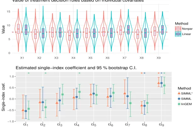
Value of treatment decision rules based on individual covariates
* * * ** *** −1.0 −0.5 0.0 0.5 1.0 α1 α2 α3 α4 α5 α6 α7 α8 α9 Single−inde x coef . Method SIMML* SIMML linGEM
Estimated single−index coefficient and 95 % bootstrap C.I.
Figure 2.6: Top row: Violin plots of the estimated values of ITRs based on each of the individual predictors x1, . . . , x9, determined from univariate nonparametric and linear re-gressions, respectively, obtained from 500 randomly split testing sets (with higher values preferred). Bottom row: The estimated single-index coefficientsα1, . . . , α9, associated with the covariatesx1, . . . , x9. The associated 95% confidence intervals obtained from BCa boot-strap with 500 replications are illustrated. Estimated significant coefficients are marked with∗ on the top.
time estimating D on the training set and computing (2.22) from the testing set. We reported the averaged values. The last three columns of Table 2.1 show the estimated index coefficients (α) obtained by two different SIMMLs and the linear GEM (linGEM) method. The SIMML can be made more efficient by incorporating a main effect component
β>D(X) in the model, i.e., we consider E(Y |T =t, X=x) = βTD(x) +gt(α>x), for an appropriate vector-valued function D(X). If the n×q matrix D is the evaluation of D(X) on the sample data, then for each α, the profile loglikelihood under this extended model (with Gaussian outcome), up to constants, is Q∗(α) = k(In−Sα) ˜Yk2, where ˜Y =
In−(In−Sα)D DTD−1DT
Y. In this analysis, we tookD(X) =X. We refer to this approach as “main effect adjusted” profile likelihood SIMML and denote it by SIMML*.
In Figure 2.5, the estimated pairs of link functions are plotted against the approach-specific single index variable, obtained from applying the two SIMML approaches and the linear GEM approach. The shapes of the regression curves capture a nonlinear treatment-by-index interaction effect, especially due to some non-monotone relationship between the index in the outcome in the drug group. In Figure 2.6, the coefficient estimates from each of those single index-based methods, and the associated 95% confidence intervals obtained from a bias-corrected and accelerated (BCa, [DiCiccio and Efron, 1996]) bootstrap with 500 replications are presented. The estimated single index coefficients reflect the relative importance of the baseline covariatesx1, . . . , x9 in determining a composite treatment effect modifier, α>X, that is used for defining the ITRs.
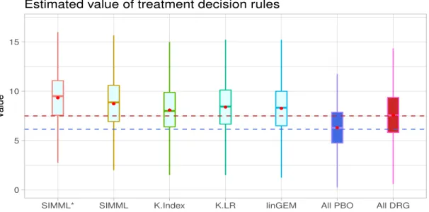
In this analysis, the incorporation of the “main effect” component improved the value of ITRs determined from the proposed SIMML method, as illustrated in the boxplots in Fig-ure 2.7; we compared the two SIMML approaches (SIMML* and SIMML); the linear GEM (linGEM) and the two approaches based on separate regression models for each treatment group (K-Index and K-LR), with respect to the estimated values (2.22) of the ITRs. For comparison, we also included the decision to treat everyone with placebo (All PBO), and the decision to treat everyone with the active drug (All DRG). The results are summarized in Figure 2.7.
The proposed SIMML approaches, in terms of the averaged estimated values (2.22) estimated from the aforementioned 500 randomly split testing sets, appeared to outperform
0 5 10 15
SIMML* SIMML K.Index K.LR linGEM All PBO All DRG
V
alue
Estimated value of treatment decision rules
Figure 2.7: Boxplots of the estimated values of ITRs obtained from the 500 randomly split testing sets (higher values are preferred). The estimated values (and the standard deviations) are given as follows: SIMML*: 9.34 (2.68); SIMML: 8.72 (2.68); K-Index: 8.04 (2.69); K-LR: 8.36 (2.69); linGEM: 8.22 (2.67); All PBO: 6.17 (2.63); All DRG: 7.57 (2.67). K-Index, exceeding the value estimated for the policy of assigning everyone to receive the active drug, while also outperforming linGEM andK-LR. The visualization (see Figure 2.5) indicates that the superiority of the active drug over placebo does not linearly decrease with the index, but rather, it appears to remain relatively constant to the left of the crossing point, exhibiting some nonlinear patterns. Finally, we note that the value of the treatment decision rule All PBO was lower than the value of the treatment decision rule All DRG, and that all treatment decision rules that took patient characteristics into account outperformed the decision of treating everyone with the drug (which is standard current clinical practice). In particular, the superiority the treatment decision rule SIMML* over treating everyone with the drug in terms of value was of similar magnitude of the superiority of the decision to treat everyone with the drug versus treating everyone with placebo. This is a clear indication that patient characteristics can help treatment decisions for patients with depression, and the more flexible SIMML methods are well suited for developing ITRs.