Lipscomb

Forestry & Natural-Resource Sciences Last Correction: Aug. 28, 2010

GEOPROCESSING SOLUTIONS DEVELOPED WHILE

CALCULATING HUMAN FOOTPRINT

STATISTICS FOR

ZONES REPRESENTING PROTECTED AREAS AND ADJACENT

LANDS AT THE CONTINENT SCALE

Donald J Lipscomb

,

Robert F Baldwin

,

1_{Res./Dem. For.,}2_{Res. Assist. Prof., DFNR, Clemson University, Clemson, SC 29634 USA}

Abstract. We calculated the mean Human FootprintTM (HF) for 196,498 polygons representing state and federally administrated ”protected areas” (e.g., National Forests, National Parks, State and Provincial Parks, etc.) of Canada, Mexico, and the Continental United States. Separate sets of calculations were made for (1) the area in each protected area which ranged in size from less than one to over 11 million hectares and (2) the area outside and within 10 km of each protected area. We used Last of the Wild version 2 (2005) for North America as the source of data for HF values. This paper concerns the technical problems we encountered using ArcGIS 9.3 and Spatial Analyst to accomplish this task in a timely manner. We developed several scripts to automate processes and address overlapping polygons resulting from zone calculations of 10 km around each protected area (doughnut-shaped polygons defining the zones from which to calculate average HF values adjacent to protected areas). We learned that Spatial Analyst does not honor the object integrity of overlapping polygons when using them to define zones for calculating zonal statistics from a raster database. We tried alternative solutions, including the use of Hawth’s Analysis Tools version 3.27 (Zonal Statistics ++) and writing scripts in Visual Basic 6.0 (VBA) to separate overlapping polygons and to calculate zonal statistics both as a table and output raster database. One of the four scripts resulting from this project was developed to calculate the 10 km zone around each protected area polygon. This script can be used to calculate a separate ‘doughnut’ polygon for any distance outside of any size polygon, even if it shares boundaries with other polygons. We also discovered that theZonal Statistics function in Spatial Analyst does not calculate all of the zones in a large database even if the polygons do not overlap. Our solution for this problem is described in this paper as an iterative process ending with another custom script to define the raster value located under the label point of each polygon in a vector database. Ultimately, we successfully calculated the mean HF from a spatially defined raster database both inside and outside the nearly 200,000 polygons defining the boundaries of Protected Areas in North America ( http://cec.org/atlas ).

Keywords: Conservation biology, geographical analysis, geoprocessing, scripts

1

Introduction

Despite their limited global coverage (15 percent of terrestrial area, and 4 percent of marine area (WDPA 2009)), protected areas have been the primary means of conserving biological diversity worldwide. At the same time, little is known about how effective their management regimes are, or in other words, how their management regimes match the intent of protected area establishment (Parks and Harcourt 2002; Rodrigues et al. 2004).

Studies examining levels of human activity in and

around protected areas have been used to assess how well protected area management is meeting biodiversity conservation goals (e.g., Parks and Harcourt 2002). We undertook such a study for the North American conti-nent using two publicly available databases. First, in 2008 we updated the North American Protected Ar-eas database using the Commission for Environmen-tal Cooperation (CEC) database, which is available at http://cec.org/atlas. The database consisted of infor-mation submitted and independently posted by the gov-ernments of Mexico, Canada, and the United States

Lipscomb et al. (2010)/Math. Comput. For. Nat.-Res. Sci. Vol 2, No 2, pp. 138–144/http://mcfns.com 139

and is an expansion both in extent and richness of a North American database produced nearly a decade ago (DellaSala et al. 2001). The 2008 North Ameri-can data contained vector data (polygon boundaries) of areas protected by state or federal government agen-cies of each country and data found to be in com-mon in their respective databases, plus IUCN (Interna-tional Union for Conservation of Nature) category codes from the World Database for Protected Areas (WDPA). While the WDPA includes a subset of all protected areas (113,959 for the entire globe), the CEC North American database is much more inclusive. The WDPA includes most GAP 1 and GAP 2 lands from the United States (e.g., National Parks and other lands managed for biodi-versity), but excludes most GAP 3 lands (multiple use). Therefore the North American database has 196,498 polygons resulting from fine-scale mapping and inclu-sive definitions primarily in the United States (PAD-US 2009).

The purpose of assembling the North American pro-tected areas database was to facilitate the making of maps and to foster communication and cooperation on environmental issues between the countries on the North American continent. However, this database presents some unique opportunities for analysis of environmen-tal issues that transcend our national boundaries. For example, we calculated the percent of ecoregions at dif-ferent levels that are protected. In this paper we will discuss the process of analyzing the pressures on these protected areas by looking at the Human FootprintTM

(HF) values inside and outside of them.

As a source of georeferenced human impact informa-tion, The HF is a global, unique source that transcends commonly used single metrics such as road and pop-ulation density. It is a multivariate index, intended to reflect a continuum of human influence normalized by each terrestrial biome (maximum values in a biome are assumed to be the maximum human activity that biome will allow). The HF is published on the Inter-net as raster data by a combined effort of the Wildlife Conservation Society (WCS) and the Center for Inter-national Earth Science Information Network (CIESIN) at Columbia University as a measure of human im-pact. The HF is based on geographic data describing human population density, land transformation, access, and electric power infrastructure in an index ranging 0-100 (Sanderson et al. 2002).

In some countries the HF, along with other measures of human influence, is used to evaluate areas to help de-cide if they should be protected (Meerman 2005). In most of North America this kind of geographic informa-tion was not available when our nainforma-tional parks and other protected areas were designated. We wanted to use the HF to compare human activity in protected areas on

the North American Continent to human activity in a 10 km area around the outside of those protected areas. We hoped to gain insight about how well protected areas are insulated from human influence and which protected areas need additional protection.

What we anticipated might be a simple analysis using Zonal Statistics functions (e.g., ESRI’s ArcGIS tools in Spatial Analyst (http://www.ESRI.com)), actually took three months and several custom scripts to accomplish. Our goal is thus to describe and discuss the difficulties met and solutions we devised during this process. While we focus on geoprocessing, we also provide results of the protected areas analysis as a means of providing con-text and as an example of a meaningful application of iterative zonal statistics.

2

Methods

2.1 Analysis of Protected Areas We initially used theZonal Statistics function in the Spatial Analyst ex-tension contained in the ArcGIS toolboxes to calculate a spatial statistics table for the protected area poly-gons mapped for the North American continent. Zonal Statistics calculates statistics on values of a raster (grid) database within the zones of another database. Each protected area polygon (in a shapefile) was used to de-fine a zone for which the statistics were calculated for the HF raster database (after converting to a raster format in ESRI GRID) contained in that zone (the specific HF version we used was Last of the Wild version 2). How-ever, this process produced results for only a majority of the protected areas, not all of them. After initial pro-cessing, we added a field to the protected area database for the mean HF value and initiated it with a -1 value (0 through 100 were legitimate values). We then popu-lated that field for records that produced real mean val-ues in the initial run. Next, we selected and exported all records that retained a value of -1, for further processing. We applied the Zonal Statistics tool to these exported polygons of protected areas and transferred the result-ing values to the protected areas database. This process was repeated until the Zonal Statistics tool produced no more new values. Polygons with no cells in them would retain a value of -1 in the final database; how-ever, some of the polygons that remained were found to have raster cells within their boundaries. A script was developed in VBA to obtain the value of the raster cell that corresponded to the position of the label point for the remaining polygons, and these values were used as a mean.

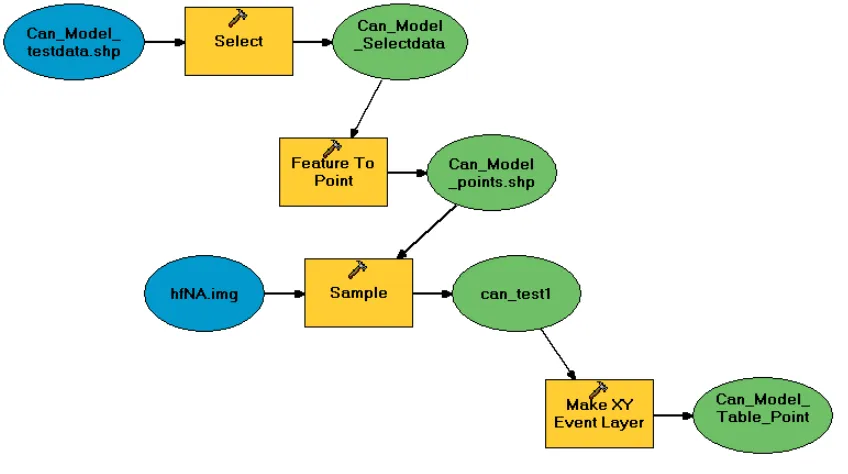
Figure 1: Geoprocessing steps illustrated using Model Builder and programmed in VBA to extract the raster database value under the label point in the associated protected area vector database polygons.

converted to points that fell within the polygon and those point locations were used to extract the values. This process is illustrated in Figure 1 using Model Builder. Model Builder is a means of organizing work-flow of geoprocessing within ArcGIS. Geoprocessing can be a complex series of input databases, tools, and out-put databases. Model Builder organizes these steps into a workflow that may be used as a tool for re-peated use. The Model Builder structure uses a test database (i.e., Can Model testdata) which represents the larger continental one. The model shows the selec-tion of the records that remain after the spatial statis-tics tools calculated mean values until it could produced no new ones (Can Model Selectdata). Next, the Fea-ture to Point tool was used to convert these remain-ing zones to points within the polygons, producremain-ing the layer ‘Can Model points’. This point layer is used with the Sample tool to extract values from the HF raster database (hfNA) and store them in a stand-alone table. The values in the table are then transferred back to the protected area database or made into a point layer and linked to the protected area database. A VBA script was developed and used in its place to streamline this process. Specifically, the script allowed us to update records in the original database during the processing of individual features instead of updating the feature layer

using a separate table or point database.

2.2 Analysis of the Zone Surrounding Protected Areas The first step in calculating the mean HF for the 10 km area around each protected area polygon was to define those zones by drawing a buffer polygon of that area without the protected area in the center. It was ap-parent we needed to perform several operations on each polygon feature as a separate object. The procedure used was to select each protected area polygon, buffer it, and then subtract (get the difference) the original polygon from the resulting buffer polygon. This pro-duced a ‘doughnut like’ polygon that defined the 10 km area around each protected area. The resulting ‘dough-nut like’ polygons often overlapped each other because of the close proximity of the protected areas. Each ‘dif-ference’ polygon was assigned a unique record number in common with the original polygon buffered. Each ‘difference’ polygon was then used to define a zone for the calculation of the zonal statistics values for the HF raster database.

ev-Lipscomb et al. (2010)/Math. Comput. For. Nat.-Res. Sci. Vol 2, No 2, pp. 138–144/http://mcfns.com 141

ident that the areas of the zones used to extract the spatial statistics did not approximate the areas of the original doughnut polygons defining those zones. We hy-pothesized that this was due to the overlap produced by drawing 10 km zones around polygons that were within 10 km of each other. Further investigation revealed this to be true: we discovered it as ArcGIS polygon (vector) databases defining the zones for theZonal Statisticstool are rasterized prior to defining the zones. Since raster databases cannot overlap in a single database, the in-tegrity of the overlapping polygons was lost, and the areas of overlap original to the polygon file were not in-cluded in the analysis by theZonal Statistics tool.

2.3 Analysis using Hawth’s Tools Because of the shortcomings of the Spatial Analyst Zonal Statistics tool, our attempts to use Model Builder to automate this task failed. We needed a tool that performed several operations on each object and used the geometry of the whole object. In our search for a tool that would honor the individual object integrity of each ‘difference’ poly-gon in defining the zone of the HF raster database to be used for calculation, we tried several tool sets developed by independent authors. Hawth’s Tools appeared to be the most promising, as the documentation suggested it honors the object integrity of overlapping polygons.

Hawth’s Tools includes aZonal Statistics ++process that is much faster than the Spatial Analyst tool because it uses code that does not work through the Spatial An-alyst extension. We applied the Zonal Statistics ++ tool to the protected area database for North America and to the 10 km zones around each. In fact, the tool was much faster than our script, taking only 3-7 days to run each analysis. However, this process produced nu-merous errors of unknown origin, resulting in valid data for only a little over 50 percent of the zonal polygons in our database. While Hawth’s Zonal Statistics ++ tool was not a completely satisfactory solution, it pro-duced a large number of values that validated our own program’s results and thus proved a useful adjunct to our own script. The error-free values from Hawth’s tool were eventually compared to the corresponding values from our VBA scripts to validate those calculations.

2.4 Using a VBA Script The solution for our anal-ysis objectives was to develop a VBA script (available upon request from the authors) that selected each pro-tected area ‘difference’ polygon one at a time and used it as the polygon to define the zone for calculating the spatial statistics of the corresponding portion of the HF raster database. There were several time-consuming steps in the process, such as finding the specific location of a polygon in the continental scale raster database and then defining that polygon’s zone as a raster database.

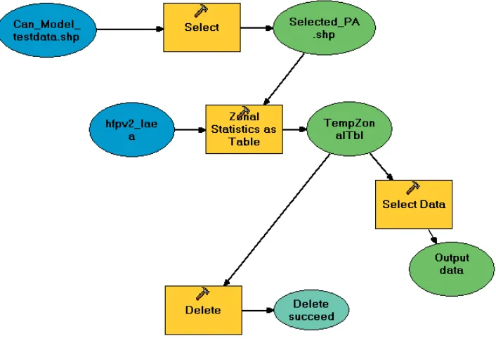
Since we needed raster database area and the zonal mean, we first placed the zonal statistics output in a single record table, then the desired values were copied from that single record table to the appropriate fields added to the protected area polygon database. After the mean and area values were transferred, the temporary table was deleted to prevent overrunning the workspace. Figure 2 illustrates this process using Model Builder. Specifically, the Select tool is used to select one pro-tected area doughnut (illustrated as Selected Pa.shp). Next the Zonal Statistics as Table tool gets the mean value from the HF raster database using selected poly-gon in raster format to define the zone. The resulting table (TempZonalTbl) with a single record in it is used to store and pass the desired values back to the pro-tected areas database. Finally, the TempZonalTbl is deleted and the next protected area doughnut polygon is selected to repeat the process.

As we suggested, the geoprocessing activity was time-consuming, requiring approximately 16 seconds to com-plete one calculation on the computer we were using (a typical desktop with a 2.33 MHz processor, 2 Gb of RAM, local storage, etc.). We calculated that process-ing all of the 196,498 protected area polygon doughnuts in this way would take 1.2 months of uninterrupted run time to complete. After several attempts, the program was modified to allow calculations to be continued start-ing at the next record after an unexpected interruption, thus allowing us to add to any progress already achieved. Since such interruptions are not discovered until the next working day, often after a delay of several days, the en-tire processing of the 196,498 records took slightly more than two months to accomplish.

2.5 Validating the Results During processing in-terruptions and after several processing steps, the raster database areas were compared to the vector polygon ar-eas to ensure that whole ‘doughnut’ polygons were used for the zonal statistics calculations. Also, results cor-responding to calculations previously completed with Hawth’s Tools were compared for assurance the results were reasonable. This trial and error process combined with the writing of the scripts, processing, and validation took more than three months to complete. The results produced mean HF values for both the protected area polygons mapped for the North American Continent and the 10 km area around each.

3

Results

Figure 2: Geoprocessing steps to obtain zonal statistics for the area outside within 10 km as repeated for multiple protected area polygons.

level codes (GAP and IUCN). While it is beyond the scope of this paper to present a full description of the protected area results, we provide a summary because they illustrate the utility of the zonal-type analyses and the geoprocessing solutions we provide above.

In summary, we found no statistical difference between impacts inside and adjacent to protected area polygons. Mean HF scores inside polygons (20.2689) were no differ-ent (α= 0.05) from those in 10 km adjacent zones (mean HF = 20.1772; t = 1.79; p = 0.0735; df = 392,994). Likewise, we found that nearly a quarter (24.5 percent) of protected area had a greater HF score on the inside than in an adjacent 10 km zone and that these ratios were related to GAP and IUCN classes. Predictably, the highest protection levels (GAP 1 and IUCN I-II) had the lowest incidence of impacts that were higher inside rather than adjacent to protected areas.

4

Discussion

Zonal analyses such as those we present here are ideal for assessing impacts to biodiversity in protected areas using abstract data such as the HF or naturalness de-rived from land cover data. So many new protected ar-eas are being added globally that conservation biologists need rapid assessment tools to evaluate how well these areas are meeting their management goals. For exam-ple, the most recent PAD US database for the United

States alone contains more than 750,000 vector poly-gons and it includes only a few private land easements (PAD-US 2009). The World Database on Protected Ar-eas (WDPA) provides data suggesting an exponential growth in the number of protected areas since the late 1800’s (<5 to 114,000). Many nations are staking the future of their biodiversity on this protected area net-work, yet there is considerable doubt as to how well the network is performing to achieve biodiversity protection goals (Margules and Pressey 2000).

To assess impacts, we need geoprocessing tools that are systematic, repeatable, and quantifiable. The WDPA (2009) provides a tool (Rapid Assessment of Land Use Change in and Around Protected Areas) to visualize land cover change inside and outside protected areas. However there are several drawbacks to their ap-proach: (1) the WDPA is a coarse filter for protected areas (we mapped nearly 200,000 polygons for North America while the WDPA 2009 presents only 16,212), (2) the land cover layer they present is not a quantified, multivariate index, like the HF, but rather is a change visualization tool, and (3) tree cover is the variable mod-eled, which does not help in assessing impacts in natu-rally open areas such as grasslands and deserts.

Lipscomb et al. (2010)/Math. Comput. For. Nat.-Res. Sci. Vol 2, No 2, pp. 138–144/http://mcfns.com 143

We encountered significant problems when using pre-defined tools (both ArcGIS 9.3 Zonal Statistics, and Hawth’s Tools version 3.27Zonal Statistics ++). These problems had to do with the treatment of overlapping buffer polygons (10 km adjacent zones) as independent objects, or errors associated with very large batch pro-cessing. We found that writing our own scripts in VB 6.0 to automate this process was the most time-efficient, and suggest that these scripts could be slightly modified for any similar zonal statistics problem.

As with any modeling process, it is important to moni-tor and validate the results. We discovered through iter-ative examination of outputs when using ArcGIS Zonal Statistics that the statistics were not being calculated for whole buffer polygons as we hoped, but only for non-overlapping portions. Likewise, we discovered many failed calculations when running Hawth’s Tools Zonal Statistics ++process by repeatedly examining attribute table outputs.

Finally, in terms of park management, our results of the HF impacts inside and adjacent to North Ameri-can protected areas has produced more questions than answers. Other analyses from around the world have pointed to human population infringement upon the bor-ders of protected areas (Parks and Harcourt 2002; Wit-temyer et al. 2008; Woodroffe and Ginsberg 1998). We expected greater levels of impact in zones adjacent to North American Protected Areas, as has been found in the tropics and associated with some mammalian extinc-tions in North America (Parks and Harcourt 2002). In some cases (e.g., heavy-use National Forests or Bureau of Land Management lands), we expected to find areas with greater impacts inside rather than outside. Yet we were surprised to find so many protected areas with greater levels of human activity inside rather than on the outside, and in particular were surprised that so many (up to 10 percent) of the areas with the highest pro-tection levels (e.g., National Parks) had greater impacts inside their boundaries rather than in the 10 km adja-cent zones. We hypothesize that where there are more impacts inside relative to outside the protected areas, parks are embedded in more extensive areas of multiple use land. National parks and other high-recreation ar-eas have a great deal of hard infrastructure very similar to urban development (e.g., paved roads, visitor centers, facilities management buildings) inside their boundaries, whereas surrounding multiple use lands may have some resource extraction activity, but little or no hard infras-tructure has been introduced.

5

Conclusions

GIS zonal statistics are useful and necessary for as-sessing impacts to protected areas. Adjacent impacts in

particular are important in assessing the ecological isola-tion of protected areas (e.g., Parks and Harcourt, 2002). However, zonal statistics tools found in ArcGIS (Spatial Analyst) or Hawth’s Tools (Zonal Statistics ++) are not efficient for large databases because using them requires close supervision of the process and results. We do not know how large a database can become before some of these problems begin to occur. Scripting tools (e.g., in VB 6.0 or Python) allow automated runs through large databases (e.g., this one was of North American extent with millions of cells and almost 200,000 features) and will honor object integrity of overlapping buffers.

However, even when the scripting tools seem to work errors may occur. There are several known sources of er-ror, therefore we offer means of identifying those below. And, there may be other currently unknown sources of error when processing large databases that should be sought before accepting the results of such analyses. We suggest:

1. Compare the raster database area from the statis-tics table to the associated vector database area for the same record in the attribute table for each poly-gon defining a zone. The two values should be sim-ilar but because cell size will influence raster area calculations relative to polygons areas, examine a number of polygons to determine percent accuracy, and then use that level tolerance when comparing raster database and vector database (polygon) ar-eas.

2. Insure that the units in the projection of the raster database and the projection of the associated vector database are the same. If they are not, then make them the same, and recalculate areas.

3. Low cell counts in zonal statistics can produce er-rors, so for zones with low cell counts, calculate some of the key statistics by hand and compare these with the outputs.

4. Examine the output for each zone (vector record) to locate missing statistical values.

surrounding rural and multiple use areas. Our results in-dicate that park infrastructure (e.g., paved roads, park-ing lots, headquarters, and concessions) can heavily out-weigh the activities in surrounding rural and multiple use areas. We need to keep in mind that the metric (the HF) may not be the best means of answering these ques-tions. For example, the metric may be too coarse, or may introduce bias in the impact weighting system. Alterna-tively, the implications may be real and protected areas may really be impacted as indicated by this analysis.

Acknowledgements

We thank the Commission for

Environmen-tal Cooperation North American Atlas Program (www.cec.org/naatlas) for their generous financial sup-port and participation in the research. In particular we thank Jessica Levine, Karen Richardson, and Tom Ham-mond of the CEC, Jim Strittholt of the Conservation Biology Institute, and Steve Trombulak of Middlebury College for their insight and suggestions. Such work would not be possible without the Wildlife Conservation Society (WCS) and the Center for International Earth Science Information Network (CIESIN) Human Foot-print methodology and data. Finally we acknowledge the Department of Forestry and Natural Resources and Public Service Activities at Clemson University. In addition, we thank two anonymous reviewers of this manuscript for their thoughtful comments.

References

DellaSala, D.A., N.L. Staus, J.R. Strittholt, A. Hack-man, and A. Iacobelli. 2001. An updated protected areas database for the United States and Canada. Nat-ural Areas Journal. 21: 124-135.

Margules, C.R., and R.L. Pressey. 2000. Systematic con-servation planning. Nature. 405: 243-253.

Meerman, J.C. 2005. Belize protected areas

pol-icy and system plan: RESULT 2 protected

area system assessment & analysis. Protected Areas Systems Plan Office (PASPO). Available at: http://biological-diversity.info/NPAPSP.htm. Ac-cessed December 16, 2009.

PAD-US. 2009. Protected Areas Database

of the United States. Available at:

http://www.protectedlands.net/padus/. Accessed December 16, 2009.

Parks, S.A., and A.H. Harcourt. 2002. Reserve size, local human density, and mammalian extinctions in U.S. protected areas. Conservation Biology. 16: 800-808.

Rodrigues, A.S.L., S.J. Andelman, M.I. Bakarr, L. Boi-tani, T.M. Brooks, R.M. Cowling, L.D.C. Fishpool, G.A.B. da Fonseca, K.J. Gaston, M. Hoffman, B.B. King, J.S. Long, P.A. Marquet, J.D. Pilgrim, R.L. Pressey, J. Schipper, W. Sechrest, S.N. Stuart, L.G. Underhill, R.W. Waller, M.E.J. Watts, and X. Yan. 2004. Effectiveness of the global protected area net-work in representing species diversity. Nature. 428: 640-643.

Sanderson, E.W., M. Jaiteh, M.A. Levy, K.H. Redford, A.V. Wannebo, and G. Woolmer. 2002. The human footprint and the last of the wild. BioScience. 52: 891-904.

Wittemyer, G., P. Elsen, W.T. Bean, A. Coleman, O. Burton, and J.S. Brashares. 2008. Accelerated human population growth at protected area edges. Science. 321: 123-126.

Woodroffe, R., and J.R. Ginsberg. 1998. Edge effects and the extinction of populations inside protected areas. Science. 280: 2126-2128.