Paper 16-2012-1

(UDC: 539.22:004.021)

On a recursive algorithm for avoiding mesh distortion in inverse form

finding

S. Germain1*, P. Steinmann1

1_{Chair of Applied Mechanics, Friedrich-Alexander-University Erlangen-Nuremberg,}

Egerlandstr.5, D-91058 Erlangen, Germany [email protected] [email protected] *Corresponding author

Abstract

A challenge in the design of functional parts is the determination of the initial, undeformed shape such that under a given load a part will obtain the desired deformed shape. A shape optimization formulation might be used to determine the initial shape in the sense of an inverse problem via successive iterations of a direct mechanical problem. In this paper, we present a shape optimization formulation for elastoplastic materials with a constitutive model for anisotropic additive elastoplasticity in the logarithmic strain space. A discrete sensitivity analysis is performed and gives the analytical gradient of the objective function needed in the optimization algorithm. We found that the use of the coordinates of the functional component as design variables led to mesh distortions. Without a split of the total force applied on the component and an update of the undeformed configuration between two steps the optimization algorithm is not able to find an appropriate minimum. Three numerical examples in isotropic and anisotropic elastoplasticity illustrate the structure of such a recursive algorithm for avoiding mesh distortions.

Keywords: inverse form finding, shape optimization, elastoplasticity, anisotropy, large strain

1. Introduction

The determination of the initial, undeformed shape such that under a given load a part will obtain the desired deformed shape is inverse to the standard (direct) kinematics analysis in which the undeformed shape is known and the deformed unknown. Inverse methods are useful tools and allow conceiving designs in less time and at lower costs than those involved with experiments or direct computational design.

extended the formulation in Govindjee et al. (1996) to the case of anisotropic hyperelasticity. They wrote the constitutive equations in terms of Lagrangian variables, i.e. Piola-Kirchhoff stresses in terms of Green-Lagrange strains. Germain et al. (2010a,b) extended the method originally proposed by Govindjee et al. (1996) to anisotropic hyperelasticity that is based on logarithmic (Hencky) strains. This work was further extended to anisotropic elastoplasticity in Germain et al. (2011a). They showed that the inverse mechanical formulation in elastoplasticity can be used if the plastic strains are previously given. This is the case when a desired hardening state is given.

Shape optimization in a sense of an inverse problem via successive iterations of a direct mechanical problem allows to determine the undeformed configuration of a functional component knowing the deformed shape, the loading and the boundary conditions. Fourment et al. (1996) suggested a shape optimization method for non-linear and non-steady-state metal forming problem. Shapes are described using spline functions. The finite-element (FE) method, including remeshing, is used for the simulation of the process. Naceur et al. (2004) proposed a new numerical approach to optimize the shape of the initial blank in deep drawing of thin sheets. This new approach is based on the coupling between the inverse approach used for forming simulation and an evolutionary algorithm. Germain et al. (2011b) proposed a numerical shape optimization method for anisotropic elastoplastic materials that is based on logarithmic strains. The objective function that needs to be minimized in order to obtain the optimal undeformed workpiece is the quadratic difference between the node positions in the target and computed (current) deformed shape, i.e. the node coordinates of the FE-domain are chosen as design variables (nodes-based optimization). A discrete sensitivity analysis is presented and analytical gradients are performed. They used the Limited-memory Broyden-Fletcher-Goldfarb-Shanno (L-BFGS) optimization algorithm proposed in Schmidt (2005) in theirs illustrations. In Germain et al. (2011c) the inverse mechanical formulation proposed in Germain et al. (2010) and the shape optimization proposed in Germain et al. (2011b) have been compared in terms of computational costs for the determination of the initial shape in hyperelasticity. They found that when dealing with hyperelastic materials the inverse mechanical formulation is more efficient than the shape optimization formulation. In Germain et al. (2012) an algorithm which updates the reference configuration during the optimization is added to the shape optimization formulation presented in Germain et al. (2011b) in order to avoid mesh distortions in metal forming processes.

The paper is organized as follows: In section 2 we introduce the notations by presenting the kinematics of geometrically non linear continuum mechanics. The third section gives a constitutive model for isotropic and anisotropic additive elastoplasticity in the logarithmic strain space based on Miehe et al. (2002) and de Souza Neto et al. (2008). The next section resumes the formulation of a direct mechanical problem needed in the inverse problem formulation. Section 5 presents a discrete sensitivity analysis and generalizes the algorithm for avoiding mesh distortions presented in Germain et al. (2012). Three numerical examples for isotropic and anisotropic elastoplastic material illustrate the recursive algorithm presented in the previous section.

2. Kinematics of geometrically non linear continuum mechanics

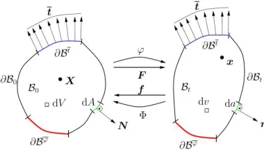
Let denote the undeformed (material) configuration of a continuum body parameterized by material coordinates X with respect to Cartesian basis at time t=0. is the corresponding deformed (spatial) configuration parameterized by spatial coordinates x with respect to Cartesian basis at time t, as depicted in Fig.1. Subsequently the bases and

body resp. , where neither Dirichlet ( ̅) nor Neumann ( ̅) data appears. is defined as a unit vector at X directed along the outward normal to an material surface element ̅_{. ̅ represents a given traction per unit area on the Neumann boundary in the material and}

spatial configuration. The direct deformation map

( ) (1)

gives the position of each spatial point in function of its material counterpart .

Fig. 1. Material (right) and spatial (left) motions.

The corresponding deformation gradient is given by

. (2)

In an index notation the direct deformation gradient tensor is expressed by

∑ , (3)

where lowercase indices refer to spatial Cartesian coordinates and uppercase indices refer to material Cartesian coordinates. The Jacobian determinant of the direct deformation gradient, which describes the local change of the volume to the deformation, is considered as positive

_{. (4)}

The inverse deformation map

( ) (5)

gives the position of each material point as a function of its spatial counterpart . The corresponding inverse deformation gradient is given by

. (6)

In an index notation the inverse deformation gradient tensor is expressed as

∑ . (7)

The Jacobian determinant of the inverse deformation gradient is assumed to be positive

_{. (8)}

From the above definitions it follows that the inverse deformation map denotes a nonlinear map inverse to the direct deformation map

Thus the inverse and direct deformation gradients together with their Jacobian determinants are simply related through an algebraic inversion

_{. (10)}

3. Constitutive model for anisotropic additive elastoplasticity in the logarithmic strain space

In this section we summarize the work by Miehe et al. (2002) and de Souza Neto et al. (2008). The constitutive phenomenological model for anisotropic additive elastoplasticity in the logarithmic strain space mimics the small strain theory and is focused on metal plasticity. An additive decomposition of the logarithmic (Hencky) strain into an elastic and a plastic part is assumed

, (11)

where

(12)

is the right Cauchy-Green tensor. The Clausius-Duhem inequality, on which the development of the constitutive model is based,

̇ ̇ , (13)

defines the local dissipation of the model with respect to unit volume. The total free energy density is decomposed into an elastic and a plastic part

( ) ( ) ( )

( ) ( ) ( ) . (14)

The elastic part is defined as a quadratic free energy density in terms of the second-order elastic strain tensor and a constant elastic fourth-order material tensor

( ) . (15)

The plastic part of the total free energy density is modeled by nonlinear isotropic hardening, i.e. kinematic hardening is not considered,

( ) _{( ) ( )( ) , (16)}

where α is a scalar that models isotropic hardening, h is the hardening modulus, ζ0 is the initial yield stress, ζ∞ is the infinite yield stress and w is the saturation parameter. T in Eq. 13 is the current stress tensor work-conjugate to the logarithmic strain measure E defined by

( ) ( ) ( ) . (17)

Considering Eq. 11 and 14 the reduced dissipation inequality can be written by

̇ ̇ . (18)

Plastic flow occurs only on the yield surface

which represents a hypersurface. A quadratic yield function or level set function (Hill-type criterion)

( ) √ √ ( ( )( _{)) (20)}

allows to define whether elastic straining or plastic yielding occurs. To model plastic incompressible flow as for metals, the plastic metric in Eq. 20 has to satisfy

. (21)

For the usual isotropic von-Mises elastoplasticity

_{. (22)}

A specific formulation of in the special case of an orthotropic response is presented in Miehe et al. (2002). The tensor defined in the Voigt notation is governed by nine parameters. In a Cartesian coordinate system aligned to the axes of orthotropy the tensor appears in the simple coordinate representation

[ ]

. (23)

Eq. 21 is satisfied for the three dependencies

( ) ( ) ( ) . (24)

Orthotropic plastic yielding for incompressible plastic flow is governed by six material parameters related to the initial yield stresses with respect to the principal axes of orthotropy

(25)

. (26)

Setting and ⁄√ is equivalent to Eq. 22 for isotropic plastic yielding. An alternative of the formulation presented in Miehe et al. (2002) to define the fourth-order tensor is the use of Kelvin modes (Sutcliffe (1992)). For the case of a cubic representation, might be defined in function of three parameters , and and three projection tensors , and as

. (25)

The variables , and are the eigenvalues of tensor expressed in the Voigt notation. The principle of maximum plastic dissipation gives the following plastic flow rule and hardening law

̇ ̇_√ ̇ √ ̇ . (27)

̇ ( ) √ ̇( ( ) √ ) (28)

allow to determine the plastic parameter. A radial-return mapping is used for solving the elastoplastic problem as in de Souza Neto et al. (2008) and Simo et al. (1998).

4. Determining the deformed shape from equilibrium

In this contribution we omit distributed body forces and inertia henceforth. The direct mechanical formulation uses a Piola formulation for the equilibrium. The following boundary value problem is solved

( ) , (29)

̅ ̅_,

̅ ̅_.

( ) denotes the material divergence operator with respect to the material coordinates X. The weak form of the given boundary value problem, with the test function on the boundary surface ̅, reads

( ) ∫ ∫ ̅ . (30)

Eq. 30 is the common virtual work statement with a parameterization of all quantities in the material coordinates X. The (symmetric) Piola–Kirchhoff stress is expressed as

(31)

The corresponding linearization (directional derivative) of the weak form in the direction at fixed material coordinates X, as needed in a Newton type solution scheme, is finally expressed as

( ) ∫ . (32)

The fourth-order tangent operator decomposes into the material tangent operator

(33)

and a geometrical contribution

[ ̅̅̅ ] [ ̅̅̅ ] ̅̅̅ . (34)

In Eq. 33 when elasticity occurs and when plasticity occurs (Miehe et al. (2002)). In Eq. 34 Iand idenote the material and spatial unit tensors with coefficients and

, respectively, ̅̅̅ denotes a non-standard dyadic product with ̅̅̅ and

I,J,K,L,i,j =1...3. For the finite element solution the discretization formulation proposed in Germain et al. (2010) is adopted.

5. Shape optimization

5.1. Discrete sensitivity analysis

Shape optimization theory allows to predict the original shape of a functional component by iterating a direct mechanical formulation. The objective function (Eq. 35), which has to be minimized in order to find the solution, i.e. the undeformed shape, is defined by a least-square minimization of the difference between the target and the current deformed configuration of the workpiece

( ) ‖ _{( )‖ . (35)}

The material coordinates X are considered as the design variables. The target deformed configuration corresponds to the known and given deformed configuration. The current deformed configuration is computed by a direct mechanical formulation (Section 4) with the undeformed configuration given by the optimization algorithm (for example L-BFGS). Numerical optimization algorithms are described in Nocedal et al. (2006). After setting the objective function a discrete sensitivity analysis is performed (Schwarz (2001) and Scherer et al. (2010)). The aim of the sensitivity analysis is to supply the gradients of the objective function and the constraints with respect to the design variables, which are necessary for the use of gradient-based optimization algorithms (Nocedal et al. (2006)). A restriction to unconstrained problems is achieved. Subsequently we are going trough the mathematical details for expressing the analytical gradient of the objective function in a discrete sensitivity analysis. By applying the chain rule on Eq. 35, we obtain

( )

. (36)

According to the implicit dependency of the objective function to the design variables X it follows that ( )

. (37)

The crucial step for computing the second term in Eq. 36 is the mechanical equilibrium equation (Scherer et al. (2010))

_{( ) ( ( ) )}

( ( ) ) , (38)

where rext and rint are the internal and external nodal forces. Applying the total differential on the above equation we obtain

. (39)

After a rearrangement we deduce

*

+

. (40)

Substituting Eq. 40 in Eq. 36 we obtain

( ) (

_{) *} +

, (41)

_{∫ ̂}

. (43)

In Eq. 42 P denotes the non symmetric Piola stress tensor and in Eq. 43 σ denotes the symmetric Cauchy stress tensor. In Eq. 42 and 43 the operator [ ̂ denotes contraction with the second index of the corresponding tangent operator, is an assembly operator with respect to the elements in a finite element formulation and N are the shape functions.

Remark:

Numerical gradients might also be provided to the optimization algorithm (Schmidt (2005)) by performing a finite difference. This approach is easy to implement but the numerical costs are very high. When the increment in the finite difference is not properly chosen it leads to relevant errors in the result (Schwarz (2001)).

5.2. Recursive algorithm for avoiding mesh distortions

A drawback of choosing the material coordinates as design variables is possible occurrence of mesh distortions. The optimization algorithm is not able to find appropriate minimums or gets stuck after few iterations (Fig. 2 and Fig. 3). Fig. 2a shows the target deformed configuration of a functional component in the [x1,x3] plan. The bottom of the shape is partially clamped and

forces are applied on the top of the shape. Fig. 2b shows the undeformed configuration in the [X1,X3] plan after 14 iterations of the optimization algorithm (L-BFGS), where mesh distortions

are well identified. Fig. 3a and Fig. 3b show the target deformed configuration of a functional component in the [x1,x2] and [x1,x3] plan. The left side of the shape is clamped and forces are

applied on the right side (three dimensional extension of the classical two dimensional Cook‘s cantilever). Fig. 3c and Fig. 3d show the undeformed configuration in the [X1,X2] and [X1,X3]

plan after 4 iterations of the optimization algorithm (L-BFGS), where mesh distortions are well identified.

The idea of our strategy (introduce in Germain et al. (2012) for metal forming processes) for avoiding mesh distortions is to perform successive optimizations by replacing the undeformed configuration needed in the next optimization step by the previous optimized undeformed configuration.

 At the initialization step material and optimization parameters are given. The variable TotalForce, i.e. the known total force applied on the shape, is set. A variable StepForce representing the force increment is defined as StepForce << TotalForce. Furthermore at the beginning xtarget= xcurrent= Xcurrent. A direct mechanical problem is computed with Xcurrent and the initial force Force0 according to Section 4 in the next step. The optimization then runs for step 0. At the end of this initial optimization we obtained the undeformed configuration Xoptimization for Force0.

 In the next step the new applied loading Forcen is equal to the previous force Forcen-1 augmented by StepForce. Taking the previous computed undeformed configuration Xoptimization,n-1 and the new loading Forcen, the direct mechanical formulation is running in order to obtain the current deformed configuration xcurrent,n of the shape. The optimization algorithm can now be used and will give the undeformed configuration for Forcen. This process is done until TotalForce is reached.

 In this case the undeformed configuration Xoptimization for the given total force is obtained.

Algo. 1. Strategy for avoiding mesh distortions in inverse form finding problems.

Fig. 2a. in the [x1,x3] plan.

Fig. 2c. in the [X1,X3] plan.

Fig. 3a. in the [x1,x2] plan. Fig. 3b. in the [x1,x3] plan.

Fig. 3c. in the [X1,X2] plan. Fig. 3d. in the [X1,X3] plan.

Fig. 3. Example for mesh distortions.

6. Numerical examples

elastoplastic material and a given distributed force so that the deformed shape is again a straight layer.

6.1. Traction of a bar in isotropic elastoplasticity

The target geometry of the deformed bar as well as the boundary and loading conditions are shown in Fig. 4. The dimensions of the bar is 10x10x20mm. The bottom of the bar is fixed in the three directions. The total applied distributed force TotalForce on the top of the bar is equal to 28 kN. The variable StepForce in Algo. 1 is equal to 1 kN. The domain is discretized using hexahedral finite elements with 16 elements and 45 nodes. An isotropic elastoplastic material is simulated with the material parameters in Table 1. The optimization parameters are resumed in Table 2 (lbfgs=Limited-Broyden-Fletcher-Goldfarb-Shanno). Fig. 5, 6 and 7 show the computed undeformed shape in the material configuration for the steps, where the force is equal to 10 kN, 20 kN and 28 kN in the [X1,X3] plan, respectively. To confirm the obtained

results, the direct problem was re-simulated starting with the coordinates of the computed undeformed shape with force equal to 28 kN (Fig. 7), the same boundary conditions and material parameters. The result is shown on Fig. 8 in the [x1,x3] plan with the obtained

equivalent plastic strains.

Young‘s modulus 211000 MPa Method lbfgs

Poisson‘ratio 0.3 HessianModify 1

Hardening modulus 200 MPa progTol 1.e-14

Initial yield stress 450 MPa optTol 1.e-4

Infinite yield stress 700 MPa Saturation parameter 17

Table 1. Material parameters. Table 2. Optimization parameters needed in Schmidt

(2005).

Fig. 6. ( ) in the [X1,X3] plan. Fig. 7. ( ) in the [X1,X3] plan.

Fig. 8. ( ) in the [x1,x3] plan with equivalent plastic strains [-].

6.1. Cook’s problem in isotropic elastoplasticity

The target geometry of the deformed cantilever as well as the boundary and loading conditions are shown in Fig. 9 in the [x1,x2] plan and in Fig. 10 in the [x1,x3] plan. The length L of the

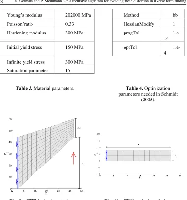
thick cantilever in is equal to 48 mm, the height H1 is set to 44 mm, the height H2 is equal to 16 mm and the width W is set to 8 mm. The left side of the thick cantilever is fixed in all directions, i.e. it is clamped. The total applied distributed force TotalForce is set to 300 N. The variable StepForce in Algo. 1 is equal to 10 N. The domain is discretized using hexahedral finite elements with 528 elements and 780 nodes. An isotropic elastoplastic material is simulated with the material parameters in Table 3. The optimization parameters are given in Table 4 (bb=Barzilai and Borwein Gradient). Fig. 11, 12, 13 and 14 show the computed undeformed shape in the material configuration for the steps where the force is equal to 10 N, 100 N, 200 N and 300 N in the [X1,X2] plan, respectively. To confirm the obtained results,

Young‘s modulus 202000 MPa Method bb

Poisson‘ratio 0.33 HessianModify 1

Hardening modulus 300 MPa progTol

1.e-14

Initial yield stress 150 MPa optTol

1.e-4

Infinite yield stress 300 MPa

Saturation parameter 15

Table 3. Material parameters. Table 4. Optimization parameters needed in Schmidt

(2005).

Fig. 11. ( ) in [X1,X2] plan.

Fig. 12. ( ) in the [X1,X2]

plan.

Fig. 13. ( ) in the [X1,X2]

plan. Fig. 14.

_{( ) in}

Fig. 15. ( ) in the [x1,x2] plan with equivalent plastic strains [-].

6.2 Anisotropic elastoplasticity

The target geometry of the deformed circular sheet with a hole in three dimension as well as the boundary and loading conditions are shown in Fig. 16 in the [x1,x2] plan. The outer radius of the

sheet in is equal to 800 mm, the inner radius is set to 400 mm and the thickness is set to 10 mm. The upper and lower surfaces are fixed in the vertical direction. The total applied distributed force TotalForce is set to 150 kN. The variable StepForce in Algo. 1 is equal to 10 kN. The domain is discretized using hexahedral finite elements with 320 elements and 720 nodes. An anisotropic elastoplastic material is simulated with the material parameters in Table 5. The optimization parameters are given in Table 6. Fig. 17, 18 and 19 show the computed undeformed shape in the material configuration for the steps where the force is equal to 5 kN, 10 kN and 15 kN in the [X1,X2] plan, respectively. To confirm the obtained results, the

direct problem was re-simulated starting with the coordinates of the computed undeformed shape at force equal to 15 kN (Fig. 19), the same boundary conditions and material parameters. The result is shown in Fig. 20 in the [x1,x2] plan with the obtained equivalent plastic strains.

Young‘s modulus 70000 MPa Method lbfgs

Poisson‘ratio 0.33 HessianModify 1

Hardening modulus 100 MPa progTol 1.e-14

Initial yield stress 450 MPa optTol 1.e-4

Infinite yield stress 715 MPa

Saturation parameter 16.5

Normal yield stress (Miehe et al. (2002)) 400 MPa

Shear yield stress (Miehe et al. (2002)) 450/√3 MPa

Schmidt (2005).

Fig. 16. in the [x1,x2] plan.

Fig. 19. ( ) in the [x1,x2] plan.

Fig. 20. ( ) in the [x1,x2]

plan with equivalent plastic strains [-].

7. Conclusion

In this paper we presented a constitutive model for anisotropic additive elastoplasticity in the logarithmic strain space. A shape optimization is formulated in the sense of an inverse problem, where the goal is to find the undeformed shape of a functional component knowing the deformed configuration, the loads and boundary conditions. In order to avoid mesh distortions, which might occur when using the node coordinates as design variables, we proposed a recursive algorithm. The computed undeformed configuration of the previous step is used in the next step for the computation of the objective function. The limitation of such a recursive algorithm is the computational time which grows when the incremental applied force is much lower than the total applied load. Three numerical examples for isotropic and anisotropic elastoplastic materials illustrated the application of this algorithm. We found that without this algorithm the optimizer is not able to find a solution for our inverse problem. Future works will be on the formulation of contact problem so that metal forming processes can be simulated and on an extension of the modeling to kinematic hardening elastoplasticity.

Извод

О рекурзивном алгоритму за избегавање кривљења мреже при

налажењу инверзног облика

S. Germain

, P. Steinmann

1

Chair of Applied Mechanics, Friedrich-Alexander-University Erlangen-Nuremberg,

Egerlandstr.5, D-91058 Erlangen, Germany

[email protected]

[email protected]

*Corresponding author

Резиме

При пројектовању функционалних делова изазов је одређивање недеформисаног облика који ће се при задатом оптерећењу деформисати у жељени облик. Формулисање оптимизације облика може бити коришћено за одређивање почетног облика у смислу инверзног проблема преко узастопних итерација директног механичког проблема. У овом раду излажемо формулацију оптимизације облика за еластопластични материјал чији је конститутивни модел адитивна анизотропна еластопластичност у простору логаритамских деформација. Примењена је дискретна анализа осетљивости која даје аналитички градијент циљне функције потребне у оптимизационом алгоритму. Утврдили смо да коришћење координата функционалне компоненте као пројектних променљивих може довести до дисторзије мреже. Без коришћења инкременталног поступка у односу на укупну силу која делује на компоненту и без ажурирања недеформисане конфигурације између два корака, алгоритам оптимизације није у стању да нађе одговарајући минимум. Три нумеричка примера изотопне и анизотропне еластопластичности илуструју структуру овог рекурзивног алгоритма за избегавање дисторзије мреже.

Кључне речи: налажење инверзног облика, оптимизација облика, еластопластичност, анизотропија, велике деформације

References

de Souza Neto EA, Periš D, Owen DRJ (2008), Computational Methods for Plasticity: Theory and Applications, John Wiley & Sons, Ltd, Chichester, UK.

Fachinotti VD, Cardona A, Jetteur P (2008), Finite element modelling of inverse design problems in large deformations anisotropic hyperelasticity, Int. J. Numer. Meth. Engng., 74, 894-910.

Fourment L, Chenot JL (1996), Optimal design for non-steady-state metal forming processes - Part I and II, Int. J. Numer. Meth. Engng., 39, 33-65.

Germain S, Steinmann P (2010b), On Inverse Form Finding For Anisotropic Materials, Proc. Appl. Math. Mech., 10, 159-160.

Germain S, Steinmann P (2011a), On Inverse Form Finding for Anisotropic Elastoplastic Materials, AIP Conference Proceedings, 1353, 1169-1174.

Germain S, Steinmann P (2011b), Shape optimization for anisotropic elastoplasticity in logarithmic strain space. In: E. Oñate, D.R.J. Owen, D. Peric and B. Suárez (Eds.),

COMPUTATIONAL PLASTICITY XI Fundamentals and Applications, 1479-1490.

Germain S, Steinmann P (2011c), A comparison between inverse form finding and shape optimization methods for anisotropic hyperelasticity in logarithmic strain space, Proc. Appl. Math. Mech., 11, 367-368.

Germain S, Steinmann P (2012), Towards inverse form finding methods for a deep drawing steel DC04, Key Engineering Materials, 504, 619-624.

Govindjee S (1999), Finite Deformation Inverse Design Modeling with Temperature Changes, Axis-Symmetry and Anisotropy, UCB/SEMM-1999/01, University of California Berkeley. Govindjee S, Mihalic PA (1996), Computational methods for inverse finite elastostatics,

Comp.Meth. Appl. Mech. Engrg., 136, 47-57.

Govindjee S, Mihalic PA (1998), Computational methods for inverse deformations in quasi incompressible finite elasticity, Int. J. Numer. Meth. Engng., 43, 821-838.

Lu J, Zhou X, Raghavan ML (2007), Computational method of inverse elastostatics for anisotropic hyperelastic solids, Int.J. Numer. Meth. Engng., 69,1239-1261.

Miehe C, Apel N, Lambrecht M (2002), Anisotropic additive plasticity in the logarithmic strain space: modular kinematic formulation and implementation based on incremental minimization principles for standard materials, Comput. Methods Appl. Mech. Engrg, 191, 5383-5425.

Naceur H, Guo YQ, Batoz JL (2004), Blank optimization in sheet metal forming using an evolutionary algorithm, Journal of Materials Processing Technology, 151, 183-191. Nocedal J, Wright SJ (2006), Numerical optimization, Springer series in operations research. Scherer M, Denzer R, Steinmann P (2010), A fictitious energy approach for shape optimization,

Int. J. Numer. Meth. Engng., 82, 269-302.

Schmidt M (2005), http://www.di.ens.fr/~mschmidt/Software/minFunc.html.

Schwarz S (2001), Sensitivitätsanalyse und Optimierung bei nicht linearem Strukturverhalten, Dissertation, Institut für Baustatik der Universität Stuttgart, Bericht Nr. 34.

Simo JC, Hughes TJR (1998), Computational inelasticity, Interdisciplinary Mathematics,

Springer, 7.