Vol. 6, No. 3; May 2019 ISSN 2332-7294 E-ISSN 2332-7308 Published by Redfame Publishing URL: http://aef.redfame.com
AR Model or Machine Learning for Forecasting
GDP and Consumer Price for G7 Countries
Yutaka Kurihara1 & Akio Fukushima2 1Professor, Department of Economics, Aichi University, Nagoya, Japan 2Researcher, Institute of Economic Studies, Seijo University, Tokyo, Japan
Correspondence: Yutaka Kurihara, Professor, Department of Economics, Aichi University, Nagoya, Japan.
Received: February 12, 2019 Accepted: March 1, 2019 Available online: March 8, 2019 doi:10.11114/aef.v6i3.4126 URL: https://doi.org/10.11114/aef.v6i3.4126
Abstract
This paper examines the validity of forecasting economic variables by using machine learning. AI (artificial intelligence) has been improved and entering our society rapidly, and the economic forecast is no exception. In the real business world, AI has been used for economic forecasts, but not so many studies focus on machine learning. Machine learning is focused in this paper and a traditional statistical model, the autoregressive (AR) model is also used for comparison. A comparison of using an AR model and machine learning (LSTM) to forecast GDP and consumer price is conducted using recent cases from G7 countries. The empirical results show that the traditional forecasting AR model is a little more appropriate than the machine learning model, however, there is little difference to forecast consumer price between them.
Keywords: AI, AR, consumer price, GDP, machine learning
1. Introduction
As AI has been increasing in many fields, machine learning has been paying much attention and is now used in many fields including economics. Ai and machine learning have gain a lot of attention in recent years and there is certainly a lot of potential for the future. Forecasting economic variables have a long history, but the statistical methods have been developing rapidly. Along with macroeconomic models, time series analysis to forecast economic variables has been conducted, and the accuracy seems to have improved. Forecasting skills have surely been increasing in spite of the fact that forecasting would be an eternal unsolvable issue. There is a lot of excellent work presented in this field.
On the other hand, new forecasting methods have been invented from AI field. AI has begun to change our society and the traditional field of economics. Policy authorities and market participants have investigated how AI would be useful or how AI should be used for economic activities. Stock prices, exchange rates, and so on are now predicted by using AI, especially in the real business world. At first, the accuracy has been quite doubtful, however, the situation has been changing gradually. Much attention has been paid to the methods using AI. There is much possibility that AI will change the economic activities, however, there is little study about the relationship between economic activities and AI performance. Such research has just begun in the academic field.
This paper examines the appropriation of forecasting economic variables by using machine learning. AI has been introduced into economics, but forecasts using machine learning have not been fully conducted. A Comparison of using AR models and machine learning to forecast GDP and consumer price is conducted in the case of recent cases from G7 countries. Whether machine learning can be better in forecasting economic data rather than traditional statistical models is examined in this paper. For economic variables, GDP and consumer price are employed as economic variables because stock prices, exchange rates, and so on, are not necessarily appropriate for machine learning as mentioned below.
Machine learning is strongly related to deep learning. Deep learning is one kind of machine learning method based on learning data. Deep learning is invented from information processing patterns or communication patterns in human nervous systems. Deep learning structures such as recurrent neural networks have been used in many ways including economics. There is not enough research whether or not the AI or machine learning using forecasting is valid.
2. Literature Review
Economics has tackled problems of forecasting for a long time. It has a long history. Zarnowitz & Lambros (1987) indicated that the relationship between survey-based dispersion and macroeconomic un-stability depends on the hypothesis that forecasters have larger influences during economic turmoil. Fair & Shiller (1990) found that the performance of economic forecasts depends on the volatility of the economy. Nalewaik (2011) showed that GDI is more appropriate than GDP for examining the economic situation. Neri & Ropele (2011) found that the estimated policy rule becomes less aggressive for inflation rates. Laurent & Andrey (2014) indicated that forecast validity of the data increases when the probability- based forecasts of the coincident indicator model and the interest rate yield curve model are combined. Chemis & Sekkei (2017) showed that the Dynamic Factor Model outperforms univariate benchmarks as well as other used now-casting models, such as Mixed Data Sampling (MIDAS) and bridge regressions. Forni, Gambetti, Lippi, & Sala (2017) found that noise shocks cause hump-shaped responses of GDP, consumption and investment, and explain a large part of their prediction error variance in business cycles. Sindelar (2017) showed that although some error patterns might indicate performance deficiencies, the validity of forecasts made by the Ministry of Finance in Czech and Czech National Bank does not differ much from the benchmark forecasting.
A lot of studies have been published recently about this field. An, Jalles, & Loungain (2018) found that forecasters know that recession periods will be different from other periods. Behrens, Pierdzioch, & Risse (2018) showed that validity of long-run inflation forecasts of four German research institutes cannot be denied and that inflation forecasting are efficient. Berge (2018) found that inflation expectations on households’ parts relate to different macroeconomic variables from the professionals’ expectations. Chan & Song (2018) indicated significant changes in the expectations, uncertainty about U.S. inflation during the Great Recession period. Dias, Pinheiro, & Rua (2018) found that factor models employing a bottom-approach for GDP is useful. Chang (2018) showed that Greenbooks (Board of Governors of the Federal Reserve System staff’s forecasts) are more likely to under-predict real GDP growth with one quarter ahead forecasts. Engstrom & Sharpe (2018) found that bond yields beyond 18 months in maturity have no added value for forecasting either boosting or recessions of GDP. Gebka & Wohar (2018) showed that the bond yield spread does not have additional information about the forecasting GDP. Lange (2018) found that the expectations component of the term spread brings more reliable forecasts of recessions than the component of the term premium in profit model. Tsui, Xu, & Zhang (2018) showed that MIDAS employing high-frequency stock return brings a better GDP forecasting than the other models, and using weekly stock returns is the best choice. Xu, Zhuo, Jiang, Liu, & Liu (2018) indicated that the Group Panelized Unrestricted Mixed Data Sampling (GP-U-MIDAS) model outperformed the other models and can choose some indicators, such as industrial production, personal consumption expenditures and so on for GDP growth forecasting.
In this study, an AR model is used for comparison along with the machine learning for G’ countries. Baker, Boom, & Davis (2016) showed uncertainty to lower GDP by 1.2%. Girardi, Golinelli, & Pappalardo (2017) found that forecasting obtained by dimension reduction methods outperformed both the benchmark AR and the diffusion index model. Kim & Swanson (2018) found that various benchmark models, including AR models, the AR models with exogenous variables, and Bayesian model averaging, do not determine specifications based on factor-type dimension reductions with various machines learning, variable selection, and shrinkage methods. Hur (2018) showed that the level of information inattentiveness about inflation has increased since the early 1980s, while a pro-cyclical information stickiness is found for GDP growth forecasts using the VAR model. Hansen, Memahon, & Prat (2017) indicated that there is increasing literature capitalizing on computational linguistics algorithms to analyze Federal Open Market Committee: US (FOMC) transcripts and other forms of central banks communication. Azqueta-Gavadón (2017) employed machine learning of natural language processing techniques. Saltzman & Yung (2018) showed that business and economic related uncertainty is related to future weakness in output, higher unemployment, and term premium by using natural language processing techniques. Swanson & Xiong (2018) indicated that big data are useful when predicting the term structure of interest rates.
This study examines the validity of forecasting economic variables by using machine learning. A comparison of using the AR model and machine learning to forecast GDP and consumer price is conducted in G7 countries. Some data, which have large fluctuations and changes in a short period, is not adequate for machine learning regardless of the data size. Machine learning examines that pattern of the data, so the data that shows a trend is adequate to analyze. GDP and consumer price seem to be adequate for comparison.
There are a lot of forecasting methods in economics. Among them, this paper employs the AR model. This method selects because it is one of the most acknowledged and traditional to forecast. Also, only one variable is used for estimation for both the AR model and machine learning. This paper’s purpose is a comparison between the two forecasting models. Arbitrage or seeming arbitrage factors or hypotheses are retrieved when conducting empirical
This paper is structured as follows. Following this section, theoretical aspects of this study are explained in section 2. Section 3 provides data description and empirical methods for the conduct of the empirical analyses. Section 4 shows the results of empirical analyses and analyzes the results. Finally, this study ends with a brief summary.
3. Methodology
The sample period is from 1992 to 2017Q3. Quarterly data are used for estimation. 1992 is selected because the Maastricht Treaty was signed in Europe in that year. That starting point is adopted in other countries. GDP growth rate and consumer price rate are used. All of the data are from International Financial Statistics by IMF. 12 data (t-12, t-11,…, t-1) are used for predicting next quarter data. The sample period is from 1992Q1 to 2017Q3, and the data of 2017Q4 are predicted. The data from 1992Q1 to 2003Q4, which is divided into almost two from the full sample period, is used for training data, and the data from 2004Q1 to 2017Q3 is used for test data. The sequential model in Keras and full sequence prediction are employed. Three interacting layers are built, and these are typical machine learning methods. Finally, this paper employs Long Short Term Memory (LSTM) instead of Recurrent Neural Network (RNN), which are developed to solve the exploding and vanishing problems that can be met when training RNNs. LSTM has been developed Instead of simple RNN in deep learning. LSTM has an advantage over RNNs. RNNs are networked with loops that allow information to persist. However, users have to pick up parameters to solve toy problems. On the other hand, LSTM is a special kind of RNN, which is capable of learning long-term dependence. This paper employs LSTM for forecasting. This is a typical method of machine learning for estimation.
4. Discussion and Analysis
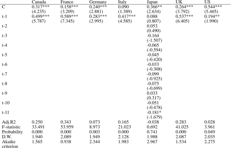
First, GDP growth rate and inflation (consumer price) rate are estimated by the AR model as shown in the following Equations (1) and (2).
GDP growth rate = c + GDP growth rate(-1) + GDP growth rate(-2) + ……..+ εt (1) Inflation rate = c + Inflation rate(-1) + Inflation rate(-2) + ……..+ εt (2) The empirical results of Equation (1) are reported in Table 1, and the results of Equation (2) are reported in Table 2. Table 1. AR model (GDP)
Canada France Germany Italy Japan UK US
C 0.317*** (4.235) 0.158*** (3.209) 0.240*** (2.881) 0.090 (1.389) 0.366** (2.634) 0.264*** (3.792) 0.544*** (5.465) t-1 0.499*** (5.787) 0.589*** (7.345) 0.283*** (2.995) 0.417*** (4.585) 0.088 (0.807) 0.537*** (6.405) 0.194** (1.990) t-2 0.053 (0.490) t-3 -0.164 (-1.507) t-4 -0.065 (-0.594) t-5 -0.045 (-0.420) t-6 -0.033 (-0.308) t-7 -0.099 (-0.925) t-8 -0.075 (-0.699) t-9 0.033 (0.317) t-10 -0.051 (-0.478) t-11 -0.181* (-1.679) Adj.R2 0.250 0.343 0.073 0.165 -0.038 0.283 0.028 F-statistic 33.491 53.959 8.973 21.023 0.692 41.025 3.961 Probability 0.000 0.000 0.003 0.000 0.741 0.000 0.049 D.W. 1.940 2.089 1.949 2.128 1.988 2.087 2.035 Akaike criterion 1.565 0.938 2.344 1.983 2.967 1.534 2.275
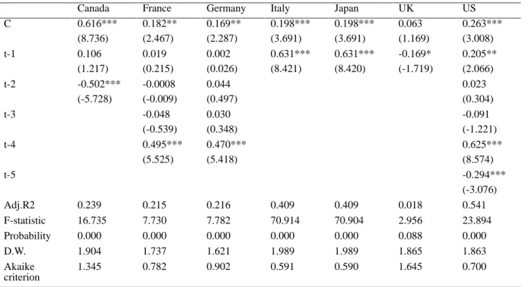
Table 2. AR model (inflation)
Canada France Germany Italy Japan UK US
C 0.616*** (8.736) 0.182** (2.467) 0.169** (2.287) 0.198*** (3.691) 0.198*** (3.691) 0.063 (1.169) 0.263*** (3.008) t-1 0.106 (1.217) 0.019 (0.215) 0.002 (0.026) 0.631*** (8.421) 0.631*** (8.420) -0.169* (-1.719) 0.205** (2.066) t-2 -0.502*** (-5.728) -0.0008 (-0.009) 0.044 (0.497) 0.023 (0.304) t-3 -0.048 (-0.539) 0.030 (0.348) -0.091 (-1.221) t-4 0.495*** (5.525) 0.470*** (5.418) 0.625*** (8.574) t-5 -0.294*** (-3.076) Adj.R2 0.239 0.215 0.216 0.409 0.409 0.018 0.541 F-statistic 16.735 7.730 7.782 70.914 70.904 2.956 23.894 Probability 0.000 0.000 0.000 0.000 0.000 0.088 0.000 D.W. 1.904 1.737 1.621 1.989 1.989 1.865 1.863 Akaike criterion 1.345 0.782 0.902 0.591 0.590 1.645 0.700
***, **, and * denote 1%. 5%, and 10% significance levels respectively.
Table 3 and Table 4 are the comparison of the AR model and machine learning (AI). Differences in Table 3 and Table 4 indicate real data minus calculated data.
Table 3. Differences between real and calculated data (GDP)
Canada France Germany Italy Japan UK US
AR 0.509 0.526 0.406 0.274 0.433 0.472 0.681 Difference -0.083 0.174 0.129 0.023 -0.214 -0.152 -0.113 Root mean squared error 0.597 0.478 0.806 0.703 0.973 0.605 0.754 AI 0.443 0.764 0.556 0.619 0.747 0.488 0.252 Difference -0.017 -0.064 -0.021 -0.322 -0.528 -0.168 0.314 Root mean squared error 0.664 0.517 1.017 0.326 1.135 0.706 0.680
Table 4. Differences between real and calculated data (inflation)
Canada France Germany Italy Japan UK US
AR 0.625 0.139 0.441 0.240 0.240 0.063 0.842 Difference -0.293 0.197 0.046 -0.536 -0.536 -0.535 -0.104 Root mean squared error 0.532 0.387 0.382 0.402 0.402 0.546 0.400 AI 0.411 0.580 0.123 0.166 0.166 0.267 0.457 Difference -0.079 -0.244 0.367 -0.462 -0.461 0.331 0.279 Root mean squared error 0.659 0.453 0.323 0.372 0.395 0.555 1.198
The empirical results are not so robust, but, they show that the AR model is a little more appropriate than machine learning, However, there is little difference to forecast consumer price between them.
5. Conclusion
This study examined the validity of forecasting economic variables by using machine learning. LSTM, as machine learning, was used for forecasting. A comparison of using the AR model and machine learning to forecast GDP and consumer price was conducted in G7 countries. Some important factors which are able to affect the forecast
used for estimation. The empirical results are not so robust, but they show that the AR model is a little more appropriate than machine learning.
Machine learning seems fitting when the data have strong trends. Prominent progress in machine learning is now ongoing, so there would be a possibility that statistical method for estimation would change somehow. There are some problems for estimating data by AI. Above all, there are no theoretical reasons. Also, causality is sometimes not clear. The word black box is sometimes used for AI, and there is some fear that such consideration is not taken into account. Wrong and inadequate beliefs and too much dependence on AI would promote turmoil in the markets. On the other hand, AI will improve rapidly as technology progresses. Forecasting economic data by AI, has only just begun. From now on, substantial progress can occur as this kind of study will be much more necessary.
Acknowledgments
We appreciate five referees for their valuable comments and suggestions on our paper. They definitely helped to improve our paper. This study was supported by the Nitto Foundation.
References
An, Z., Jalles, J. T., & Loungain, P. (2018). How well do economics forecast recessions? International Finance: 21(2), 100-121. https://doi.org/10.1111/infi.12130
Azqueta-Gavadón, A. (2017). Developing news-based economic policy uncertainty index with unsupervised machine learning. Economics Letters, 158, 47-50. https://doi.org/10.1016/j.econlet.2017.06.032
Baker, S. R., Boom, N., & Davis, S. J. (2016). Measuring economic policy uncertainty. Quarterly Journal of Economics, 131(4), 1593-1636. https://doi.org/10.1093/qje/qjw024
Behrens, C., Pierdzioch, C., & Risse, M. (2018). Testing the optimality of inflation forecasts under flexible loss with random forecasts. Economic Modelling, 72, 270-277. http://dx.doi.org/10.1016/j.econmod.2018.02.004
Berge, T. J. (2018). Understanding survey based inflation expectations. International Journal of Forecasting, 34(4), 788-801. http://dx.doi.org/10.1016/j.ijforecast.2018.07.003
Chan, J., & Song, Y. (2018). Measuring inflation expectations uncertainty using high-frequency data. Journal of Money, Credit, and Banking, 50(6), 1139-1166. https://doi.org/10.1111/jmcb.12498
Chang, A. C. (2018). The Fed’s asymmetric forecast errors. Finance and Economics Discussion Series FRB), 2018-026. https://doi.org/10.17016/FEDS.2018.026
Chemis, T., & Sekkei, R. (2017). A dynamic factor model for nowcasting Canadian GDP growth. Empirical Economics, 53(1), 217-234. http://dx.doi.org/10.1007/s00181-017-1254-1
Dias, F., Pinheiro, M., & Rua, A. (2018). A bottom-up approach for forecasting GDP in a data-rich environment.
Applied Economics Letters, 25(10), 718-723. https://doi.org/10.1080/13504851.2017.1361000
Engstrom, E. C. & Sharpe, S. A. (2018). The near-term forward yield spread as a leading indicator: A less distorted mirror. Finance and Economics Discussion Series FRB), 2018-055.
Fair, R. C., & Shiller, R. J. (1990). Comparing information in forecasts from econometric models. American Economic Review, 80(3): 375-89.
Forni, M., Gambetti, L., Lippi, M., & Sala, L. (2017). Noisy News in Business Cycles. American Economic Journal: Macroeconomics, 9(4), 122-152. http://dx.doi.org/10.1257/mac.20150359
Gebka, B., & Wohar, M. E. (2018). The predictive power of the yield spread for future economic expansions: Evidence from a new approach. Economic Modelling, 75, 181-195. https://doi.org/10.1016/j.econmod.2018.06.018
Girardi, A., Golinelli, R., & Pappalardo, C. (2017). The role of indicator selection in nowcasting Euro-area GDP in Pseudo-Real time. Empirical Economics, 53(1), 79-99. http://dx.doi.org/10.1007/s00181-016-1151-z
Hansen, S., Mcmahon, M., & Prat, A. (2017). Transparency and deliberation within the FOMC: A computational linguistics approach. Quarterly Journal of Economics, 133(2), 801-870. https://doi.org/10.1093/qje/qjx045
Hur, J. (2018). Time-varying information rigidities and fluctuations in professional forecasters’ disagreement.
Economics Modelling, 75, 117-131. http://dx.doi.org/10.1016/j.econmod.2018.06.009
Kim, H. H., & Swanson, N. R. (2018). Mining big data using parsimonious factor, machine learning, variable selection, and shrinkage methods. International Journal of Forecasting, 34(2), 339-354.
Lange, R. H. (2018). The predictive content of the term premium for GDP growth in Canada: Evidence from linear, Markov-Switching, and probit estimations. North American Journal of Economics and Finance, 44, 60-81. https://doi.org/10.1016/j.najef.2017.11.001
Laurent, P., & Andrey, V. (2014). Forecasting combination for U.S. recessions with real-time data. North American Journal of Economics and Finance, 28, 138-48. https://doi.org/10.1016/j.najef.2014.02.005
Nalewaik, J. J. (2012). Estimating probabilities of recession in real time using GDP and GDI. Journal of Money, Credit and Banking, 44(1), 235-253. https://doi.org/10.1111/j.1538-4616.2011.00475.x
Neri, S., & Ropele, T. (2011). Imperfect information, real-time data and monetary policy in the Euro area, Economic Journal, 122, 651-74. https://doi.org/10.1111/j.1468-0297.2011.02488.x
Saltzman, B., & Yung, J. (2018). A machine learning approach to identifying different types of uncertainty. Economics Letters, 171, 58-62. https://doi.org/10.1016/j.econlet.2018.07.003
Sindelar, J. (2017). GDP forecasting by Czech institutions: An empirical evaluation. Prague Economic Papers, 26(2), 155-160. https://doi.org/10.18267/j.pep.601
Swanson, N. R., & Xiong, W. (2018). Big data analytics in economics: What have we learned so far, and where should we go from here? Canadian Journal of Economics, 51(3), 695-746. https://doi.org/10.1111/caje.12336
Tsui, A., Xu, C. Y., & Zhang, Z. (2018). Macroeconomic forecasting with mixed data sampling frequencies: Evidence from a small open economy. Journal of Forecasting, 37(6), 666-75. https://doi.org/10.1002/for.2528
Xu, Q., Zhuo, X., Jiang, X., & Liu, Y. (2018). Group panelized unrestricted mixed data sampling model with application to forecasting U.S. GDP growth. Economic Modelling, 75, 221-236.
http://dx.doi.org/10.1016/j.econmed.2018.06.021
Zarnowitz, V., & Lambros, L. A. (1987). Consensus and uncertainty in economic prediction. Journal of Political Economy, 95(3), 591-620. https://doi.org/10.1086/261473
Copyrights
Copyright for this article is retained by the author(s), with first publication rights granted to the journal.
This is an open-access article distributed under the terms and conditions of the Creative Commons Attribution license which permits unrestricted use, distribution, and reproduction in any medium, provided the original work is properly cited