Upamanyu Madhow, Michael L. Honig and Ken Steiglitz†
ABSTRACT
In personal communications applications, users communicate via wireless with a wireline net-work. The wireline network tracks the current location of the user, and can therefore route mes-sages to a user regardless of the user’s location. In addition to its impact on signaling within the wireline network, mobility tracking requires the expenditure of wireless resources as well, includ-ing the power consumption of the portable units carried by the users and the radio bandwidth used for registration and paging. Ideally, the mobility tracking scheme used for each user should depend on the user’s call and mobility pattern, so that the standard approach, in which all cells in a registration area are paged when a call arrives, may be wasteful of wireless resources. In order to conserve these resources, the network must have the capability to page selectively within a registration area, and the user must announce his or her location more frequently. In this paper, we propose and analyze a simple model that captures this additional flexibility. Dynamic pro-gramming is used to determine an optimal announcing strategy for each user. Numerical results for a simple one-dimensional mobility model show that the optimal scheme may provide significant savings when compared to the standard approach even when the latter is optimized by suitably choosing the registration area size on a per-user basis. Ongoing research includes com-puting numerical results for more complicated mobility models and determining how existing system designs might be modified to incorporate our approach.
I. INTRODUCTION
The basic features of personal communications may be abstracted as follows:
(i) Mobile subscribers carrying portables can communicate via wireless with fixed radio ports which are connected to a conventional wireline network;
(ii) the wireline network keeps track of the user’s location, and can therefore route messages to a user regardless of his or her current location.
The subject of this paper is mobility tracking, which we define as the process by which the network keeps track of a user’s location between two successive calls to the user. (The term call may refer to either voice or data communications.) Tracking a user’s movements during a call is a separate task involving handoffs or automatic link transfers, and is not considered in this paper. The conventional, or registration area approach, for mobility tracking is as follows. The geo-graphical area in which a user may roam is divided into registration areas containing a number of
cells, where a cell is the coverage area of a single radio port. The network tracks the user’s
regis-tration area, not the user’s cell. When a user changes regisregis-tration area, he or she announces the new location to the network. The user does not alert the network of location changes within a registration area. When a call arrives for the user, the network pages all cells in the registration area via wireless broadcast. The user receives the paging message and responds, and the call is
*This work was presented in part at IEEE Infocom ’94, Toronto, Canada, June 1994.
† Upamanyu Madhow was with Bell Communications Research, Morristown, NJ. He is now with the Coor-dinated Science Laboratory and the Department of Electrical & Computer Engineering, University of Illinois, 1308 W. Main, Urbana, IL 61801. Michael Honig was with Bell Communications Research. He is now with the Department of Electrical Enginering & Computer Science, Northwestern University, Evanston, IL 60208. The work of Ken Steiglitz was partly supported by NSF Grant MIP-9201484.
set up.
The cost of mobility tracking depends on the expenditure of the following resources: (i) The network uses wireless resources (downlink bandwidth) for paging users;
(ii) the user’s portable unit uses power for listening to beacons broadcast by the radio ports (to detect changes in his or her own location) and for alerting the network of a location change. The latter typically has higher power requirements in addition to requiring uplink bandwidth.
If a user is not very mobile and gets frequent calls of short duration, paging all cells in the registration area for each call is likely to be wasteful of expensive wireless resources of Type (i). Such a situation may arise with the advent of wireless computing, in which case the ‘‘calls’’ may actually be bursts of data. On the other hand, keeping closer track of the user’s location involves additional expenditures of Type (ii), since the user must listen more frequently to detect smaller changes in location, and must alert the network accordingly. This paper provides a mathematical formulation which enables the optimization, using dynamic programming, of the tradeoff between resources of Type (i) and Type (ii) on a per-user basis; that is, the location strategy for each user depends on his or her individual mobility pattern and the frequency with which he or she is called. The mobility model considered is a Markov random walk, and the optimal policy is for the user to alert the network of his or her location based on a threshold rule.
Mobility tracking also imposes a significant burden in terms of signaling within the wireline network (see [1] and the references therein), and changing user location strategies to optimize power and bandwidth influences the design of the wireless signaling scheme as well. For simpli-city, however, we ignore this problem in this paper.
We have recently become aware of an approach similar to ours [3], in which the mobility model is a random walk, and users alert the network of their position according to a threshold rule based on knowledge of position, number of moves, or time. The threshold rule is assumed to determine a steady-state distribution of the position of each user, which is then used to evaluate the paging cost for a Poisson call arrival model. The key difference between our work and that in [3] is that we consider mobility tracking between calls (the user’s position must be tracked per-fectly during a call, hence there is no scope for optimization there), and therefore do not make the simplifying assumption that the user’s position evolves to a steady-state by the time the next call arrives. Our dynamic program therefore tracks the position of the user throughout an inter-call interval.
Another paper with a similar motivation is [6], which attempts to choose the registration area size on a per-user basis. However, the fluid flow model of mobility (often used for aggregate vehicular traffic in cellular applications) used in that paper may not be accurate on a per-user basis, especially for personal communications applications in which most users are likely to be pedestrians. We believe that the random walk mobility model considered here and in [3] is more realistic for such applications. In Section IV, we discuss the approach of [6] in the context of our random walk model, and indicate how the performance of this approach can be evaluated by using our dynamic programming formulation. The performance of this scheme is then compared with the performance of the expanding search scheme, in which the cost incurred due to network paging is assumed to be proportional to the distance from the user’s last known location. In con-trast, the approach in [6] assumes that all cells in a registration area are paged when attempting to locate a user, even if the user has not moved far from his last known position. Consequently, the expanding search scheme yields substantial performance improvements (at the expense of greater complexity). A random walk mobility model is also considered in [4], but the optimization of the user location strategy is not linked to the expected frequency of calls.
Finally, an aggregate user location strategy which is independent of user parameters is the
and a user alerts the network whenever he or she visits one of these cells. When a call arrives, the network pages the vicinity of the reporting center from which the user reported most recently. While optimizing the choice of reporting centers may lead to improvement over the current approach, the scheme in [2] is still a static scheme which does not exploit the possibly different call and mobility patterns for different users.
The model used for optimizing the user location strategy is presented in Section II. We give properties of the optimal strategy, including a procedure for numerically computing it by iterating the dynamic programming equation. For simplicity, the results are stated for a one-dimensional random walk model of mobility. However, as shown in the appendix, the results of Section II generalize easily to higher dimensions and more complicated mobility models. In Sec-tion III we present, for our one-dimensional example, an alternative method for obtaining the optimal strategy that is based on explicitly solving an appropriate difference equation. Numerical results which show the dependence of the optimal strategy and associated performance on call and mobility parameters are given in Section IV. As previously mentioned, the performance of the expanding search scheme is also compared with the registration approach presented in [6]. Our conclusions are given in Section V.
II. SYSTEM MODEL AND DYNAMIC PROGRAMMING EQUATIONS
Since our purpose is to devise per-user location strategies, we consider a single mobile user. The user moves according to a discrete-time model specified later. At each time, the user makes a decision whether or not to announce his or her current location to the network. The cost of each announcement is A, and may represent an expenditure of power or bandwidth. The location
X(t)∈IRM of the user at time t refers to the coordinates of the current position of the user relative to the position at the most recent announcement, and is assumed to be known to the user. If a call arrives at time t, the paging cost incurred by the network is assumed to be a nonnegative function of the user’s location, and is given by f (X(t)), where this cost would typically represent the expenditure of bandwidth. The form of the cost function is based on the assumption that the net-work starts its search for the user from the position at which the user last announced.
Since the network must track the user’s location perfectly during a call, we may assume that the user’s location is known to the network when a call terminates. Starting from such a state (X(0) = 00, where 00 denotes the origin), we want to devise an announcing policy such that the expectation of the sum of the announcing costs and the paging cost of the next call is minimized. We formulate this as a dynamic program which terminates at the (random) time of arrival of the next call. At each discrete time, the probability of call arrival is given byλ, so that the duration of the dynamic program is a geometrically distributed random variable.
The position at time t of the user is incremented by a random vector Y(t)∈IRMto obtain the position at time t+1, where the Y(t) are independent and identically distributed random vectors. This is a memoryless mobility model, since the increments in position are independent of the pre-vious motion of the user. If there is no call by time t, the user takes the action ut(X(t))∈{0,1},
where ut(X(t)) = 0 denotes not announcing, and u(t) = 1 denotes announcing. If
ut(X(t)) = 0, then X(t+) = X(t), and if ut(X(t)) = 1, X(t+) = 00, where X(t+) denotes the
user’s location immediately after the decision. Thus,
X(t+1) = Y(t) , X(t) + Y(t) , ut(X(t)) = 1. ut(X(t)) = 0, (1)
Given the user’s location at time 0, if the next call arrives at time T, the expectation of the sum of the announcing and paging costs is given by
Vu(X(0)) = E
{
t
Σ
=1T
Aut(X(t)) + f (X(T))
}
, (2)where u = (u1, u2, . . . ) is a collection of functions ut, each mapping IRM to the action space
{0,1}. Since the mobility tracking is assumed to start after the termination of a call, we are pri-marily interested in minimizing Vu(00), since X(0) = 00. However, the optimal policy actually
minimizes V(r) for all r∈IRM.
Since the call arrival process and the mobility model are both memoryless, and since the paging cost function f depends only on the location X(t) (and not on the time t), it suffices to con-sider stationary policies which depend only on the user’s location, that is, ut(X(t)) = u(X(t)),
and u = (u, u, ...).
The preceding model is fairly general, in that the dimension of X(t) and Y(t), the distribu-tion of Y(t), and the dependence of the paging cost f on X(t), may be arbitrary. Under these gen-eral assumptions, we show in the appendix that an optimal policy exists and that it can be com-puted via an iterative algorithm. A similar iterative algorithm may be used to compute the cost of any stationary policy as well. For simplicity of presentation, however, we consider a discrete-space, one-dimensional random-walk mobility model for the remainder of this section, and reword some of the general results of the appendix in this context. The remaining sections of this paper also focus exclusively on this simple mobility model.
One-dimensional mobility model
We assume that the user moves according to a symmetric one-dimensional random walk; that is, letting Y denote a random variable with the same distribution as Y(t), we have
Y = −1, +1, 0, with probability with probability with probability q, q, p, (3)
where p + 2q = 1. Proposition 1 supplies a characterization of the optimal policy and its cost, and Proposition 2 gives an iterative method for computing it. The proofs of these propositions are given in a more general setting in the appendix. We denote the one-dimensional position X(t) by r.
Proposition 1: For the preceding model, the optimal policy u*(r) and the cost V*(r) are unique, and are given by
u*(r) = 1, 0, V*(r) = A + V*(0) , V*(r) < A + V*(0) , (4a) V*(r) = min
{
λ[p f (r)+q f (r−1)+q f (r+1)] + (1−λ)[pV*(r)+qV*(r−1)+qV*(r+1)] , A+V*(0)}
, (4b) where r = 0, ±1, ±2, . . . .For r = 0, the minimum is achieved by the first term on the right-hand side, so that u*(0) = 0 and
V*(0) = λ[p f (0) + q f (−1) + q f (+1)] + (1−λ)[pV*(0) + qV*(−1) + qV*(+1)].
Proposition 2: The optimal cost can be computed using the iteration
Vn+1(r) = min
{
λ[p f (r)+q f (r−1)+q f (r+1)] + (1−λ)[pVn(r)+qVn(r−1)+qVn(r+1)] ,A+Vn(0)
}
, (5)where r = 0, ±1, ±2, . . . , and where the initial condition V0(r) may be any bounded function of r. Convergence is geometric and uniform in r. That is,
V*−Vn+1 ∞ ≤ (1−λ)n V*−V0 ∞ → 0, as n → ∞, where α ∞ = ∆ r
sup α(r) denotes the L∞norm ofα.
An immediate consequence of Proposition 2 is the following result.
Corollary: If f (r) is nondecreasing in r for r ≥ 0 and in−r for r ≤ 0, then the optimal policy is a threshold rule of the form:
u*(r) =
1, otherwise,
0, RL < r < RU
where RL < 0 < RU. We allow the values RL = − ∞and RU = ∞(these correspond to never
announcing). If f (r) is symmetric in r, then RL = −RU.
Proof: Let V0(r) = 0 for all r in Proposition 2. Using induction in n, it is easy to see that for each n, Vn is nondecreasing in r for r ≥ 0 and nonincreasing in r for r ≤ 0. Since Vn→V*, the optimal cost V* is also nondecreasing in r for r ≥ 0 and nonincreasing in r for r ≤ 0. From (4), the optimal rule must be a threshold rule.
We consider now the special case
f (r) = c r , (6)
where c > 0. For this symmetric cost function, we can simplify the iteration (5) by exploiting the symmetry of the mobility model (3) and deduce that V* must be symmetric in r. The itera-tion (5) need only be considered for nonnegative values of r in this case. However, in order to obtain a practical iterative algorithm, it is necessary also to limit the range of r over which the iteration (5) is executed as follows. Assuming that an upper bound V (0) for V
*(0) is available,
let Rmaxbe the minimum value of r such that
λfs(r) > A + V (0) ≥ A + V
*(0) , for all r ≥ R
max,
where fs(r) = p f (r) + q f (r−1) + q f (r+1). The existence of a finite Rmax is guaranteed for
f as in (6), since fs(r)→∞as r→∞. From (4), we see that V*(r) = A + V*(0) for r ≥ Rmax, so that u*(r) = 1 for all such r. It is therefore necessary only to consider r < Rmaxin the itera-tion (5), setting Vn(−Rmax) = Vn(Rmax) = A + Vn(0) for all n. This numerical method for computing the optimal policy applies to more general models, as shown in the appendix. Numer-ical results for the cost function (6) are presented in Section IV.
It remains to obtain an upper bound V(0). Consider the policy u(r) = 1, r ≥ 1, 0, r = 0,
in which the user announces immediately upon moving. We take the cost of this policy as our upper bound, and compute it as follows:
V(0) = λ[p f (0) + q f (−1) + q f (1)] + (1−λ)[pV(0) + 2q(A+V(0))] ,
so that
V(0) = p f (0) + q f (−1) + q f (1) + 2qA (1−λ)/λ. (7) For f as in (6), we obtain V(0) = 2q[c + A/λ], which is finite forλ > 0.
III. SOLUTION TO DYNAMIC PROGRAMMING EQUATIONS
The results of the previous section imply that, for the mobility model (3) and for any sym-metric cost function f (e.g., f given by (6)), the optimal policy must lie in the class of symsym-metric threshold rules given by
uR(r) = 1, r ≥ R, 0, r < R (8)
A specialization of Fact A1 in the appendix implies that the cost function VR(r) for the rule uR is
given by
VR(r) = λ[p f (r)+q f (r−1)+q f (r+1)]
+ (1−λ)[pVR(r)+qVR(r−1)+qVR(r+1)] , 0 ≤ r < R, (9a)
VR(r) = A+VR(0) , r ≥ R. (9b)
The cost function VR(r) is therefore a solution to the second-order difference equation (9a)
with boundary condition (9b) (the latter actually gives two boundary conditions, at r = −R and r = R). This provides the following alternative method for computing the optimal policy: solve
(9) for arbitrary R, and compute the optimal threshold R*as
R* = arg
R > 0min VR(0) . (10)
While the optimal solution minimizes VR(r) for all r, it suffices to consider r = 0 for computing
the threshold.
The remainder of this section is devoted to finding an explicit solution to (9). The cases
R < ∞and R = ∞(this corresponds to the policy of never announcing) are handled separately, since the boundary conditions (9b) are not useful for R = ∞. We notice in some of our numerical
computations that the function VR(0) is nearly constant in the region around its minimum,
which implies that using (10) to find R*can be very sensitive to roundoff error, but shows as well that the optimal expected cost in these cases is insensitive to exact choice of R*. Forλ > 0,
con-sidering R < ∞suffices for characterizing the optimal policy via (10), since it is easily seen that, if f (r) → ∞asr → ∞(as it does for f as in (6)), then the cost function V∞(r) also tends to∞
as
r → ∞. This shows that the policy of never announcing cannot be optimal. Nevertheless, the
performance of this policy serves as a useful benchmark to which the performance of the optimal policy can be compared. In our numerical results in Section IV, the performance measure is taken to be the announcing gain in using the optimal policy compared to using the policy of never announcing, defined as V∞(0)/V*(0).
Solution for a finite threshold
Fix R < ∞, and replace VR by V for notational simplicity. For r ≤ R − 1, the solution to
(9a) can be obtained in terms of V(0) and V(1). These latter quantities are then determined by the appropriate boundary conditions. Since f (r), and therefore V(r), are symmetric in r, we obtain V(1) in terms of V(0) by substituting r = 0 in (9a):
V(1) = 2(1−λ) q 1 − (1−λ) p V(0) − 1−λ λ ( f (1) + 2q p f (0)) . (11)
Now define the one-sided z-transform
V
ˆ
(z) =k
Σ
=0∞
z−kV(k) ,
and note that
k
Σ
=0 ∞ z−kV(k+1) = z(Vˆ
(z) − V(0)) (12a) and kΣ
=0 ∞ z−kV(k−1) = z−1Vˆ
(z) + V(1) . (12b)The z-transform of the paging function, f
ˆ
(z), is defined in the analogous way, and satisfies the analogous properties. Multiplying both sides of (9a) by z−r, summing from r=0 to∞, and rear-ranging gives Vˆ
(z) = − q(1−λ) λ (qz−1+p+qz) fˆ
(z) gˆ
(z) + V(0) − 2q(1−λ) 1 + 2q p + z gˆ
(z) (13) where gˆ
(z) = z2 − (1−λ) q 1 − (1−λ) p z + 1 z , (14)and where we have assumed that f (0) = 0. The sequence {V(r)} is easily obtained from (13) by using the relationships (12), and the fact that the sequence corresponding to the z-transform g
ˆ
(z) is g(i) = z+ − z− z+i − z−i , (15)where z± = 1 + 2q(1−λ) λ ±
√
λ[λ + 4q(1−λ)] (16) are the roots of the denominator polynomial in gˆ
(z), and satisfy 0 < z− < 1 < z+. The result is V(r) = λQ(r) + 1⁄2V(0)(z + r + z − r) . (17) where Q(r) = q f (1) g(r) + iΣ
=1 r g(r−i) p f (i) + q f (i+1) + q f (i−1) . (18)We now must determine V(0). Substituting r = R*−1 in (9a) shows that V(R*) is determined by V(R*−1) and V(R*−2). Since the solution to (9a) is unique, given V(0) and V(1), it follows that V(R*) must also satisfy (17). Combining (17) for r = R*with (9b) gives
V(0) = 1 − 1⁄2(z + R* + z−R*) λQ(R*) − A (19)
which relates V(0) with the chosen threshold R*. Now the expression for V(r), (17), is clearly monotonically increasing with V(0). Consequently, V(r) is minimized by choosing the integer threshold R*in (19) to minimize V(0). This completes the solution to the dynamic programming equations (9).
Solution With No Announcing
The cost function V∞(r) for this policy satisfies (9a), for all r, so that V∞(r) is again
deter-mined by (17). To determine V∞(0) in this case, we must examine the behavior of V∞(r) as
r → ∞. Consider the following problem, which is somewhat different from that posed in Section
1. If a call arrives when the user is at r, where r > 0, paging cost f (r) is incurred. Otherwise, the user always moves to r+1. Clearly, the expected paging cost for this system is greater than the expected paging cost for the original system. We therefore have the upper bound
V∞(r) ≤ ED( f (r+D)) = i
Σ
=0∞
λ(1−λ)if (r+i) (20)
where D is the random variable which represents the distance the user moves before a call arrives. If
i
Σ
=0∞
(1 − λ)if (i) < ∞ (21)
then (20) gives a finite bound on V∞(r) for all r that is independent of V∞(0). Now examining the solution (17), we see that since z+ > 1, V∞(r) increases as O(z+r) for general V∞(0). Since
z+ > 1/(1−λ), this is inconsistent with (20) and (21) unless V∞(0) is selected to eliminate the
z+r terms in (17). Equivalently, V(0) in (13) must be selected to cancel the pole at z+.
(z − z+) V
ˆ
∞(z)|z=z+ = 0 (22)From (21), it follows that f
ˆ
(z) converges for z > 1/(1−λ), so that combining (13) with (22) gives V∞(0) = − [1 − (1−λ) p] − 2(1−λ) qz+ 2λ(p + qz+−1 + qz+) fˆ
(z+) . (23)Using the fact that z+z− = 1, this simplifies to
V∞(0) = 1−λ 2λ
√
λ[λ + 4q(1−λ)] fˆ
(z+) . (24)Finally, we note that for the cost function f (r) = c r , f
ˆ
(z) = z/(z − 1)2. IV. NUMERICAL RESULTSBecause we want to compare the scheme discussed in Section II with the one introduced in [6], we first describe this latter scheme in our context. The set of announcing strategies is assumed to contain only threshold rules, as specified by (8). In the approach of [6], the network pages all nodes within a prespecified distance R from the user’s last known location. In the one-dimensional mobility model (3) considered here, this ‘‘area’’ is an interval. Rather than assume the cost function f (r)=c r , which assumes that the network pages according to an expanding
search around the last announced location, the approach of [6] assumes a cost function for paging given by
fR(r) =
∞, r ≥ R.
cR, r < R,
In the optimization framework of the previous sections, uR (see (8)) is clearly the optimal policy for the cost function fR, and the expected cost UR(r) for this policy satisfies the following
equa-tion:
UR(r) = λcR + (1−λ)[pUR(r)+qUR(r−1)+qUR(r+1)] , 0 ≤ r < R,
UR(r) = A+UR(0) , r ≥ R.
We can easily solve for UR(.) using either value iteration or the difference equation
method. We can then define the optimal cost between calls for the alternate approach by
U*(0)=
R
min UR(0). In our numerical results, we compare the gains G′ = V∞(0)/U*(0) with
G = V∞(0)/V*(0). The first quantity gives a measure of how much gain is obtained by optim-izing the registration area method, compared to a simple never-announce scheme which uses expanding search. The quantity G is a measure of the gain obtained by optimizing our scheme, again compared to the never-announce scheme. Clearly, G′may be less than or greater than one, depending on the range of parameters. However, we always have G > 1 (due to the optimiza-tion) and G > G′(optimized expanding search must be better than an optimized scheme which pages all cells in the uncertainty region).
We now present some typical numerical results, using the iterative algorithm to compute
V*(0) and (24) to compute V∞(0). We start with the case when the cost of paging is a linear function of distance r, as in (6). Since the announcing gain is a function of the ratio c/A, there are three independent parameters to consider: c/A (cost of paging relative to announcing),λ (proba-bility of call arrival), and 2q = pmoving, the probability of the user moving in one time interval.
To get some insight into the shape of this function of three independent variables, we will show three plots with each of the parameters as independent variable.
c/A, normalized cost of paging
announcing gain and critical threshold
10-1 100 101 0 2 4 6 8 10 12 14 critical threshold announcing gain lambda = 0.01, p_moving = 0.05
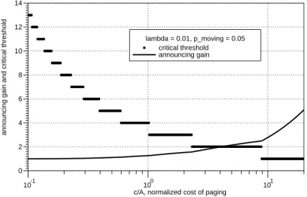
Fig. 1 Announcing gain and critical threshold versus normalized cost of paging, for the case of linear paging cost.
Figure 1 shows the announcing gain V∞(0)/V*(0) versus relative cost of paging c/A. The behavior for low and high values of paging costs is in accordance with intuition: When the cost of paging is small, the announcing threshold is large because there is no great penalty for being caught far away from the last-known position. At the same time, there is little relative advantage to announcing over never announcing, so the announcing gain falls to unity as the relative paging cost approaches zero. At the other extreme, when the cost of paging is high relative to announc-ing, the threshold drops to one, and the announcing gain increases to large values — in this case reaching 5.09 when c/A is 20. The shape of the announcing gain curve has clear discontinuities in its derivative, occurring at the points where the discrete threshold parameter jumps. The curve can be viewed as the maximum over a family of curves, one for each possible threshold value.
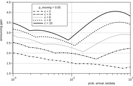
Figure 2 shows a set of curves of announcing gain versusλ, for five different values of c (A is fixed at unity with no loss of generality). As above, the curve has discontinuities in slope where the threshold changes, and each curve can be thought of as the upper envelope of a family, one for each choice of announcing threshold. It is interesting to note that high announcing gains for fixed probability of moving occur at both small and large λ, a fact that does not have an easy intuitive explanation. As expected, the optimal announcing gain always increases with increasing paging cost c.
Figure 3, the final plot for the case of linear paging cost, shows a similar family of curves of announcing gain versus probability of moving, for the same five values of c. The behavior of announcing gain versus the probability of moving is similar, except the gains are considerably larger for small probabilities of moving than for large. The announcing strategy can result in large savings when the user is not very mobile.
We next consider a paging cost with a step in cost:
f (r) =
C2, r ≥ r0,
prob. arrival, lambda announcing gain 10-3 10-2 10-1 1.0 1.5 2.0 2.5 3.0 3.5 4.0 4.5 c = 2 c = 4 c = 6 c = 8 c = 10 p_moving = 0.05
Fig. 2 Announcing gain versus probability of arrivalλ, for the case of linear paging cost.
prob. moving, p_moving
announcing gain 10-3 10-2 10-1 1 2 3 4 5 6 7 8 9 c = 2 c = 4 c = 6 c = 8 c = 10 lambda = 0.01
Fig. 3 Announcing gain versus probability of moving, for the case of linear paging cost.
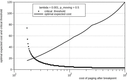
representing the situation where a fixed-cost C1 is incurred by paging within a certain radius r0, which then jumps to C2 beyond r0. Figure 4 shows the optimal expected cost V*(0) versus C2, for the value C1 = 10, a plot analogous to Fig. 1 for linear cost. It is interesting to observe that the results are qualitatively similar, with the same general pattern of decreasing critical r as the paging cost (in this case C2) increases. As C2 decreases towards C1 = 10, the cost of being paged far from the most-recently known r decreases, the critical r increases without limit, and the expected cost decreases. The plot also exhibits points of discontinuity in the derivative of the
cost of paging after breakpoint
optimal expected cost and critical threshold
101 102 103 0 20 40 60 80 100 120 critical threshold optimal expected cost lambda = 0.001, p_moving = 0.5
Fig. 4 Optimal expected cost versus normalized cost of paging, for the case of a pag-ing cost with a step.
expected cost as the threshold distance changes.
To summarize these numerical results, using the optimal announcing strategy can result in large gains in resource utilization, especially when the cost of paging relative to announcing is large and the probability of moving is small. However, dependence of announcing gain on the parameters c/A,λ, and pmoving is complex, and the relative advantage of the optimal per-user stra-tegy in particular situations is difficult to predict without numerical solution of the dynamic pro-gramming equations.
The convergence criterion used for generating all the data in the figures was that the nor-malized root-sum-square difference in V between two successive iterations be less than a prescribedε. That is, if Vj(r) is the expected cost at location r and iteration j, the criterion is that
all r
Σ
[
Vj(r)]
2 all rΣ
[
Vj(r) − Vj−1(r)]
2 1⁄ 2 < εAll the computations reported above usedε = 10−12, an array of length 300, and the final solu-tion was checked to verify that it was of the predicted form: the announcing decision ‘‘no’’ to the left of a critical r and ‘‘yes’’ to the right.
Computational experience with the iterative algorithm has shown it to be very reliable and stable. The number of iterations is quite predictable from point to point, changing slowly as the
independent parameter changes. For example, the 33 points in the range between c/A = 13 and
20 in Fig. 1 all took precisely 2,372 iterations to converge. In general, the number of iterations to
convergence is only very weakly dependent on the parameters c/A and pmoving, but is very
strongly dependent onλ. When λ = 0.1 in Fig. 2, the algorithm required only 190 iterations to converge, while whenλ = 0.001, it required 20,715 iterations.
The strong dependence of convergence time onλis predicted by the convergence analysis in the appendix. It is shown there that the method is an iterative contraction mapping, with norm decreasing as (1 − λ)k, where k is the iteration number. The number of iterations to converge to a fixedεis therefore inversely proportional to log(1 − λ) ∼∼ λwhenλis small. For example,
in the case of Fig. 2 cited above, the ratio of maximum to minimum λ is 100 while the
corresponding ratio of actual number of iterations to convergence is 109, which checks quite well.
Finally, Figure 5 shows a comparison between the gain of the registration area method in [6] and the gain corresponding to the expanding search scheme, plotted versus the probability of arrival λ, for two values of the paging cost coefficient c. The results show that the benefits of expanding search relative to the registration area approach increase with c. It also illustrates that the registration area method can achieve a gain greater than one relative to the never-announce strategy.
We conclude that optimized expanding search offers significant gains over the never-announce strategy, especially for large paging costs, but that these gains are not obtainable with the registration area method, even if its threshold is chosen optimally.
prob. arrival, lambda
gain, no-announce cost/best cost
10-3 10-2 10-1
0 1 2 3
4 registration area method, c=1expanding search method, c=1 registration area method, c=10 expanding search method, c=10
Fig. 5 Comparison between gains in the registration area and expanding search methods.
V. CONCLUSIONS
We proposed a model that captures the tradeoff between the costs of downlink paging and uplink position-announcing for tracking mobile users. We showed that the optimal choice of strategy is determined by dynamic programming equations, and proved that the equations have a unique solution under general circumstances. Further, we showed that the optimal policy is for the user to announce position when his or her distance from the previously established position exceeds a critical threshold.
Solution of the dynamic programming equations was studied in detail for a simple Markov mobility model in one-dimension, although the results mentioned above apply in much more gen-eral cases. Two approaches were presented for finding the optimal threshold. The first is an iterative algorithm based on value iteration, and the second is based on explicit solution of the
difference equation that results in this case. We showed that the iterative algorithm is a contrac-tion and converges geometrically to the unique solucontrac-tion.
We presented illustrative numerical results for the cases when the paging cost as a function of distance is linear and a step function. We also compared these results with those obtained from the registration area approach in [6]. Results show that significant gains in power and bandwidth utilization can result from the optimal announcing strategy, especially when the cost of paging relative to announcing is large, and the user is not very mobile. Comparable gains are not obtain-able with the registration area method.
REFERENCES
[1] V. Anantharam, M. L. Honig, U. Madhow and V. K. Wei, ‘‘Optimization of a database
hierarchy for mobility tracking in a personal communications network,’’ Performance
Evaluation, vol. 20, pp. 287-300, 1994.
[2] A. Bar-Noy and I. Kessler, ‘‘Tracking mobile users in wireless communications networks,’’
Proc. IEEE Infocom ’94, Paper 10b.4, San Francisco, Ca., March 1993.
[3] A. Bar-Noy, I. Kessler, and M. Sidi ‘‘Mobile users: To update or not to update?’’ Proc.
IEEE Infocom ’94, paper 5a.1, Toronto, Canada, June 1994.
[4] Y. N. Doganata, T. X. Brown, E. C. Posner, ‘‘Call setup strategy tradeoffs for universal
digital portable communications,’’ ITC Specialist Seminar, paper no. 14.2, Adelaide, 1989.
[5] H. Kushner, Introduction to Stochastic Control. New York: Holt, Rinehart, and Winston,
1971.
[6] H. Xie, S. Tabbane, D. J. Goodman, ‘‘Dynamic location area management and performance
analysis,’’ Proc. VTC ’93, pp. 536-539, Secaucus, NJ, May 18-20, 1993. APPENDIX
Our problem is one of optimal control until a desired target set (next call arrival) is reached, and this topic has been treated in depth in Chapter 4 of [5]. Due to the generality of the model considered in [5], it is difficult to obtain results for the case of continuous space and unbounded costs. The main results in [5] therefore apply to a discrete-space, bounded-cost model. By exploiting the specific features of our problem, however, we can modify the results in [5] to obtain proofs of (the analogues of) Propositions 1 and 2 when the state X(t) may be a continuous random vector, and the cost function f may be unbounded. Specialization of these results to the one-dimensional model (3) yields Propositions 1 and 2 as stated in Section III.
Before proving the desired results, a number of definitions are needed. As in Section II, we denote by X(t) the location of the user immediately prior to the decision at time t, and by X(t+) the location immediately after the decision at time t, so that X(t+1) = X(t+) + Y(t). Letting X(t) ,Y(t)∈IRM, denote by FY(z) the cumulative distribution function (cdf) of Y(t), and, for
r∈IRM, denote by Fr(z) = F(z−r) the cdf of Y(t) + r. For any functionα with domain IRM,
define Srα = ∆ E{α(X(t+1)) X(t+) = r} = IR
∫
M α(z) dFr(z) , (A.1)where E{.} denotes expectation with respect to the distribution of Y(t). For the discrete-space, one-dimensional model (3), we obtain
For any functionα, and for any stationary policy u, define
Ruα(r) =
∆
P[call does not arrive at t+1] Eu{α(X(t+1)) X(t) = r}. (A.2)
where Eu{.} is expectation with respect to the controlled Markov chain defined by u and the dis-tribution of Y(t). Using (1) and (A.1), the function Ruα is obtained fromα by the following
linear transformation: (Ruα)(r) = (1−λ) S00α, u(r) = 1. (1−λ) Srα, u(r) = 0, (A.3) Lettingα ∞ = ∆ r
sup α(r) denote the L∞ norm ofα, it is clear from (A.1) that Srα ≤ α ∞.
Thus,
Ruα ∞ ≤ (1−λ) α ∞ , (A.4)
so that Ruis a contraction mapping.
Next, define the modified paging function fs(r) as the expectation of the paging cost if a
call arrives at time t+1, given that X(t+) = r after the decision u(X(t)). We have
fs(r) =∆ E{ f (X(t+1) X(t+) = r} = Srf .
Define a modified cost function Ku(r) by
Ku(r) =
∆
P[call arrives at time t+1] Eu{ f (X(t+1) X(t) = r} (A.5)
= A + fs(00) , fs(r) , u(r) = 1, u(r) = 0,
The function Ku(r) is potentially unbounded if the modified paging cost fs(r) is unbounded. In
the latter instance, we may, as in the example in Section II, restrict r to a bounded region D by considering only stationary policies for which
u(r) = 1, r ∈/ D, (A.6)
where D is chosen to be large enough to ensure that the optimal policy satisfies (A.6), and such that fs(r) is bounded for r ∈ D. This implies, in turn, that the modified cost function Ku is
bounded for all r. The choice of D for a given cost function f is specified later (if f is bounded,
we may take D = IRM). For the one-dimensional example in Section II, the region D was
characterized as D = {r: r < Rmax}.
From (A.2) and (A.5), it is clear that the expected cost-to-go Vu(r) for any stationary rule u is given by:
Fact A1: The solution to (A.7) is finite and unique for any stationary rule u satisfying (A.6), and
can be computed using value iteration as follows:
Vun+1 = Ru Vun + Ku,
where Vu0 is an arbitrary bounded function.
Proof: Iterating on (A.7), we obtain Vu = i
Σ
=0∞
Rui Ku, a sum which is easily seen to converge
using (A.4) and the boundedness of Ku as follows:
i
Σ
=0 ∞ RuiKu ∞ ≤ Ku ∞ iΣ
=0 ∞ (1−λ)i < ∞.Uniqueness also follows from (A.4): if V and V
˜
are solutions to (A.7), then V−V˜
= Ru(V−V˜
),so that V−V
˜
∞ ≤ (1−λ) V−V˜
∞, which implies that
V−V
˜
∞ = 0 or V = V
˜
. To prove convergence of the value iteration, we note thatVun+1 = Run Vu0 + i
Σ
=0 n Run Ku. Since Run Vu0 ∞ ≤ (1−λ)n Vu0 ∞ → 0 by (A.4), we have Vun+1 → iΣ
=0 ∞ Rui Ku as required.Fact A1 characterizes the performance of any stationary policy u in the class of interest. The optimal policy is now characterized as follows.
Fact A2: The optimal solution is the unique solution of V* =
u
min (RuV + Ku) , (A.8)
and can be computed using the value iteration
Vn+1 =
u
min (RuVn + Ku) , (A.9)
where V0 is an arbitrary bounded function.
Specializing Fact A2 to the one-dimensional mobility model (3) yields Propositions 1 and 2.
Proof: To prove uniqueness, letting V and V
˜
denote two solutions to (A.8) corresponding to deci-sion rules u and u˜
, respectively, we haveV = RuV + Ku ≤ Ru˜V + Kv˜, V
˜
= Ru˜V˜
+ Ku˜ ≤ RuV˜
+ Ku,Ru(V−V
˜
) ≤ V−V˜
≤ Ru˜(V−V˜
) .Using (A.4), this implies that V−V
˜
∞ ≤ (1−λ) V−V
˜
∞, which proves V = V
˜
.To prove optimality, letting V*, u*denote the solutions to (A.8), for any policy u, we have
V* = Ru*V* + Ku* ≤ RuV* + Ku = Vu,
where u = (u, u*, u*, ...). Iterating, we obtain that for u = (u1, ..., un, u*, u*, ...),
V* ≤Vu = Run . . . Ru1V* + Kun +
i
Σ
=1n−1
Run . . . Rui+1Kui.
Since the first term on the extreme right-hand side tends to zero as n→ ∞ by (A.4), we have
V* ≤ Vufor any policy u.
Finally, to prove the convergence of value iteration, let un be the policy achieving the minimum in (A.9) at the nth iteration. Then
Vn+1 = RunVn + Kun ≤ Ru*Vn + Ku*,
V* = Ru*V* + Ku* ≤ RunV* + Kun. We obtain, therefore, that
Ru(V*−Vn) ≤ V*−Vn+1 ≤ Run(V−Vn). Iterating, we obtain Run(V*−V0) ≤ V*−Vn+1 ≤ RunRun−1 . . . Ru0(V−V0) , so that V *−Vn+1 ∞ ≤ (1−λ) n V *−V0 ∞ → 0, as n → ∞,
proving convergence of the value iteration (A.9).
It remains to specify the domain D in (A.6). For this, assume, as in the one-dimensional example in Section II, that an upper bound V (00) for the optimal cost is available. Define D to be
the smallest domain such that
λfs(r) > A + V (00) ≥ A + V
*(00) , for all r ∈/ D.
In order to satisfy (A.8), we must have u*(r) = 1 for r ∈/ D, so that we may restrict attention
to policies satisfying (A.6) without loss of generality. In order to obtain a finite upper bound V (00) for V
*(00), consider the ‘‘always announce’’
policy in which u(r) = 1, r ≠ 00. 0, r = 00, (A.10)
announcing cost A is incurred, and the location is reset to 00. While an exact expression for the cost V(00) of this policy was obtained for the one-dimensional mobility model in Section II, in general, it suffices to consider the following upper bound on V(00) which applies regardless of the mobility model.
V(00) ≤ A (1−λ)/λ + fs(00) . (A.11)
Forλ > 0, this provides a finite upper bound for V*(00) as long as fs(00) < ∞. If the latter con-dition is not satisfied, clearly the optimal cost cannot be finite either (assuming λ > 0), since fs(00) is the minimum paging cost that can possibly be incurred when the next call arrives. If
λ = 0, the optimal policy is, of course, the ‘‘never announce’’ policy u(r) = 0 for all r, since the next call never arrives, and the optimal cost V* = 0.
To see why (A.11) is true, let N be the number of announcements by the time the next call arrives, and let T be the time of arrival of the next call. By virtue of our discrete-time model, there is at most one announcement in one time unit, so that N ≤ T. The cost of the policy (A.10)
is therefore bounded as follows:
V(00) ≤ A E{N} + fs(00) ≤ A E{T} + fs(00) = A (1−λ)/λ + fs(00) .