Clock Synchronization using Packet Streams
?Philipp Blum?? and Lothar Thiele
Institut f¨ur Technische Informatik und Kommunikationsnetze ETH Z¨urich, ETH Zentrum, CH-8092 Z¨urich, Switzerland
E-mail:{blum,thiele}@tik.ee.ethz.ch
Abstract. Recent distributed applications in the domains of digital audio and sensor net-works require clock synchronization in the order of 10µs. The achievable precision depends on system properties like synchronization message delay and synchronization message pattern. These properties are often unknown or difficult to determine. Therefore we propose a new analysis for clock synchronization algorithms. The analysis is based on two properties: safe
synchronization andoptimal selective synchronization. We present two algorithms that use an
arbitrary stream of synchronization messages to achieve clock synchronization over an
asyn-chronous communication channel and on clocks with unknown and variable drift. The first
algorithm needs no parameterization, is safe and optimal selective. The second algorithm im-proves the first with a drift compensation mechanism. It is safe. A parameter of the algorithm allows to choose between fast drift compensation and high probability of optimal selective behavior. Simulation results show that the algorithms can achieve 10µs precision on 802.11b wireless LAN in ad-hoc mode.
1 Introduction and Related Work
Recent distributed applications in the domain of high-quality digital audio require clock synchronization between nodes in the order of 10µs. Similar precision requirements in the context of sensor networks have been reported by [6]. Tight synchronization is difficult because of clock drift and non-deterministic message delay. Another limiting factor is the amount of communication spent on synchronization. Several probabilistic clock synchroniza-tion algorithms have been proposed to achieve a good precision under partially unknown system specifications. [3, 1, 9] use a client-server approach to read reference time repeatedly until this succeeds with a specified precision bound. [3] achieves a precision in the order of 1ms using 4 messages per minute, [1] is similar. [9] achieves 1µs using highly determin-istic Myrinet communication. The drawback of client-server schemes is that they do not scale well with system size and synchronization message frequency. A producer-consumer approach is taken in [2]. With unidirectional communication only, a precision in the order of 1ms is achieved. This approach requires that statistical properties of the message delays are known. For broadcast networks, [5] proposes a scheme that eliminates the medium ac-cess time from the synchronization path and achieves precision in the order of 10µs using commercial off-the-shelf technology.
Unknown system properties like non-deterministic message delay and synchronization message pattern make it difficult to apply bounds on the achievable precision as proposed by [8, 7, 10, 12, 11]. Therefore we propose an analysis of clock synchronization algorithms under completely unknown system specifications in terms of message delay and message pattern. Instead of bounds on the achievable precision, we propose two properties that describe “good” algorithms. Safe synchronization never degrades the precision of a synchronized clock. Optimal selective synchronization never misses to improve the precision if there is a chance to do so. As a consequence, the achieved precision can only improve when more communication is spent on clock synchronization. We propose two new algorithms. The first algorithm needs no parameterization, is safe and optimal selective. The second algorithm
?
This work has been developed in cooperation with BridgeCo AG, Ringstrasse 14, 8600 D¨ubendorf, Switzer-land
??
The author has received funding from the Swiss Commission for Technology and Innovation (KTI), Effin-gerstrasse 27, 3003 Bern, Switzerland
improves the first in that it compensates clock drift. It is safe. A parameter of the algorithm allows to chose between fast drift compensation and high probability of optimal selective behavior. We evaluate the algorithms based on real network and clock traces, obtained in a 802.11b wireless LAN network in ad-hoc mode and standard Linux PCs.
Our assumptions on communication and clocks are similar to those of [8, 12, 11]. Our system model is different from [3, 1, 9] that assume a client-server synchronization algorithm with communication in both directions . It is different from [2] in that we make no statistical assumptions on message delay distribution. It is different from [5] in that we do not require a broadcast medium, though our producer-consumer scheme is also directly applicable in a broadcast system. Our algorithms are similar to Lamport’s algorithm for physical clocks [8]. They are different in that they start software clocks that progress always slower than
reference time.
Presentation overview: In section 2, we introduce a model for clock synchronization
algo-rithms that use streams of synchronization messages. Section 3 introduces the properties
safe synchronization and optimal selective synchronization and presents thelocal selection
algorithm. In section 4, we present the local selection algorithm with drift compensation. Section 5 presents simulation results based on real network and clock traces.
2 System model
The system we study in this paper is distributed to two nodes: On the first node, a process that has access to reference time generates synchronization messages. Reference time is assumed to be a positive real number t ∈ R≥0. We refer to this node and the associated
process as the synchronizationsource orproducer. The second node has no direct access to reference time but it can read a local hardware clock that has an arbitrary offset and an unknown and variable drift relative to reference time. We refer to this node as the synchro-nizationconsumer. Upon every arrival of a synchronization message, a clock synchronization algorithm is invoked on the consumer.
2.1 Communication
Definition 1. A Synchronization message is a tuple (s, r) where s ∈ R≥0 represents
its send time, i.e. reference time at the moment when the message is sent at the producer
node, and where r ∈R≥0 represents receive time, i.e. reference time at the moment when
the message is received at the consumer node. The payload of a synchronization message
includes at least its send time. The delay of a message is the difference between its send
and receive time, i.e. d def= r−s. The delay of a synchronization message is positive, i.e.
d >0.
Definition 2. A Synchronization streamis an infinite sequenceS def= h(si, ri)|i∈N≥1i
of synchronization messages received by the consumer, ordered by their receive time, i.e.
∀i∈N≥1:ri < ri+1.
Messages can get lost in the communication channel: The index i only counts those synchronization messages that eventually reach the consumer. Messages can get reordered in the channel: The index i counts the synchronization messages in their order of arrival, which is not necessarily the order in which they are produced.
2.2 Clocks
The consumer node has access to a read-only hardware clock h. The clock synchronization algorithm computes a new software clock ci whenever it is executed. An application that
requires synchronization always reads the software clock that has been started last. Software clocks are a well known concept [13, 4] and are also known under the name oflogical clocks.
Definition 3. The Hardware clock is a monotone increasing and differentiable function
h:R≥0 7→R≥0 that maps all values of reference time t to clock time h(t). The drift of the
hardware clock is a function ρh : R
≥0 7→ R that maps all values of reference timet to h’s
derivation minus 1:
ρh(t)def= dh(t)/dt−1. (1)
Assumption 1 The drift of the hardware clock is bounded by the known constant
ρh
max. The first derivation of the drift is bounded by the known constant δmaxh .
∀t∈R≥0 :|ρh(t)|< ρhmax ∧ |dρh(t)/dt|< δhmax. (2)
Definition 4. A Software clock is a monotone increasing and differentiable function
ci : R≥0 7→R≥0 that maps values of reference time t to clock time ci(t). The function ci is
computed at time t=ri and its domain is {t∈R≥ri}.
The index i expresses that the software clockci(t) is started in the i-th execution of the
synchronization algorithm. The drift of the software clock functions is defined as ρi(t) def
= dci(t)/dt−1 and the precision asi(t)
def
= ci(t)−t. We will use the shortcuts ci def = ci(ri), i def = i(ri),ρi def = ρi(ri) andρhi def = ρh(r
i). These definitions apply analogously toc0i, ρ0i and
0
i used in section 4.
2.3 Clock synchronization algorithm
Upon the reception of the synchronization message (si, ri), the consumer invokes a clock
synchronization algorithm. The input for this algorithm is the payload of the synchroniza-tion message, i.e.si and a timestamp from the local hardware clockhi =h(ri). The output
is a new software clock ci(t), which is supposed to be synchronized to reference time. The
algorithm has access to memory to retrieve information that has been stored in previous executions. This allows the algorithm to use the current value of all previously started software clocks cj(ri), j < iin its computation of the new software clock.
3 Analysis of clock synchronization using streams
We have made no assumptions on communication except that messages arrive after they have been sent. Therefore it is not possible to calculate a finite bound on the precision a clock synchronization algorithm can achieve. Instead, we propose properties that describe a “good” algorithm and try to find implementable algorithms for which these properties hold under the assumptions made in the previous section.
3.1 Safe clock synchronization Definition 5. Safety
A clock synchronization algorithm is safe if in all executions except the first, it starts a
software clock with an initial precision that is equal to or better than the precision of the previously started software clock at this time:
∀i∈N>1:|i| ≤ |i−1(ri)|. (3)
The probabilistic algorithms are not safe. [3, 1, 9] select updates if the measured bound
on the precision is better than a configured threshold. However this condition does not imply that the precision itself improves by the update. [2] updates the clock after a fixed number of synchronization messages have been received. Thus a better precision of the new clock reading is only probable but not guaranteed.
Definition 6. ASelective synchronization algorithmis a clock synchronization
algo-rithm that calculates a candidate initial value˜ci∈R≥0and a decision selecti∈ {true,false}.
The new software clock is started with the initial value ci:
ci := ˜ ci if selecti =true ci−1(ri)if selecti =false (4) We have found a selective clock synchronization algorithm that is safe for all synchro-nization streams:
Definition 7. The Local selection algorithm is a selective synchronization algorithm with:
˜
ci:=si, (5)
selecti:= (i= 1)∨(si > ci−1(ri)), (6)
ci(t) :=ci+ (1−ρmaxh )(h(t)−hi). (7)
The precision of the candidate initial value is defined as ˜i def
= ˜ci −ri. In the case
of the local selection algorithm, it is ˜i = si −ri = −di, which is always negative. The
algorithm only then selects a candidate initial value if it is ahead of the current software clock. Equations (5) and (6) correspond in essence to Lamport’s algorithm [8]. In addition, the local selection algorithm assures by (7) that the drift of the software clockci(t) is always
negative.
Proposition 1. The local selection algorithm is safe.
Proof. We have to show that if a candidate initial value is selected, it does not degrade
precision, i.e. selecti → |˜i| ≤ |i−1(ri)|. From (6) we get selecti→si > ci−1(ri). Therefore,
si −ri > ci−1(ri)−ri and ˜i > i−1(ri). Since 0 > ˜i > i−1(ri), we get |˜i| ≤ |i−1(ri)|,
which is what we wanted to prove.
Since the proof did not require (7), Lamport’s algorithm is also safe. 3.2 Optimal selective clock synchronization
There exists also a trivial algorithm that is safe: Start all new software clocks with the current reading of the previously started software clock ci =ci−1(ri). Though safe, this is
obviously not a good clock synchronization algorithm. Therefore we complement the safety property by a second property that a synchronization algorithm should fulfill:
Definition 8. Optimal selective
A selective synchronization algorithm is optimal selective if in all executions, it starts a
software clock with an initial precision that is equal to or better than the precision of the candidate initial value:
∀i∈N≥1:|i| ≤ |˜i|. (8)
The property is true if an algorithm never misses to improve the precision if it has the
chance to do so. The property does not hold for [3, 1, 9] because updates are selected on
the base of the precision bounds and not the precision itself. Different interpretations are possible for [2]: The property is either not defined if the algorithm is executed only after the required number of messages have been received or it does not hold, if the algorithm is executed upon every message arrival and only selects an update in fixed intervals.
Proof. We have to show that all candidate initial values that have not been selected would have degraded precision, i.e. ¬selecti → |˜i| ≥ |i−1(ri)|. From (6) we get ¬selecti → ˜i ≤
i−1(ri). To conclude our proof we have to show that i−1(ri) is negative. Since i−1(ri) =
i−1+
Rri
ri−1ρi−1(t)dtand∀t∈R≥ri−1 :ρi−1(t) =ρ
h(t)−ρh
max <0, we geti−1(ri)< i−1. By
(5),(6) and (4), we know thati−1 =max(˜ci−1, ci−2(ri−1))−riand thusi−1< max(0, i−2).
Together with the anchor 1 = ˜1 <0, this proves that ∀i∈N≥1 :i<0 by induction.
This algorithm makes always the right decisions even though it knows neither the preci-sion of the candidate initial value ˜i nor that of the current value of the previously started
software clocki−1(ri). This is possible, because the software clock and the candidate initial
value are both always behind reference time. Then it suffices to select only those candidate initial values that are larger and therefore closer to reference time than the current reading of the previously started clock. The algorithm of Lamport [8] is not optimal selective, be-cause if the consumer clock is ahead of reference time and its drift is positive, the algorithm will never select updates anymore and the precision degrades forever.
The drawback of the local selection algorithm is that in three out of four cases, the absolute value of the software clock drift is larger than the drift of the hardware clock, assuming equal probability distribution of ρh(t) in the interval
−ρh
max, ρhmax
. 4 Drift compensation
In this section we extend the local selection algorithm presented in the previous section with a drift compensation mechanism.
Definition 9. The Local selection algorithm with drift compensation is a selective synchronization algorithm that uses the same expressions as the local selection algorithm
for the candidate initial value ˜ci (5) and the decision selecti (6). Additionally it calculates
the drift compensation term βi, using the parameter b. A modified software clock c0i(t) is
started at time t=ri:
βi:=
−ρh
max if i= 1
max{βi−1−δmaxh (hi−hi−1), βi,j|j∈N≥1, j < i}otherwise
(9) βi,j :=βj+ ˜ ci−c0j(ri) (hi−hj) − b (hi−hj) −2δmaxh (hi−hj), (10) c0
i(t) :=ci+ (1 + max(βi−1/2δmaxh (h(t)−hi),−ρhmax))(h(t)−hi). (11)
Without looking at the drift compensation mechanism, we can state that,
Proposition 3. The local selection algorithm with drift compensation is safe.
The proof of proposition 1 applies directly to the algorithm with drift compensation, since both algorithms use the same ˜ci and selecti.
But what about optimal selectivity? The proof of proposition 2 required that the current reading of the previously started clock has a negative precision. This is guaranteed if the drift of all software clocks is always negative. The drift of the modified software clock is
ρ0
i(t) =ρh(t) + max(βi−δhmax(h(t)−hi),−ρhmax), (12)
and by assumption 2 smaller than its initial value, i.e. ρ0
i(t)< ρ0i. If it can be shown that the
initial driftρ0
i is always negative, then the local selection algorithm with drift compensation
is optimal selective.
After the first execution with β1 =−ρhmax, the modified software clock is the same as
that from (7). In later executions, the drift compensation term βi is set to the maximum
compensation of the previously started clock βi−1 −δmaxh (hi−hi−1). The potential drift
compensation termsβi,j are computed based on the comparison of the new candidate initial
value ˜ci with the current reading of the previously started software clock c0j(ri)|j < i.
Compared toβj, the drift compensation termβi,jcan be increased by (˜ci−cj0(ri))/(hi−hj),
but is decreased by b/(hi−hj) + 2δhmax(hi−hj). The parameterb is a constant, therefore
it decreases βi,j most for software clocks c0j(t) that have been started only recently (small
hi−hj). The term 2δhmax(hi−hj) has the opposite effect: Clocks that have been started a
long time ago can not be used for drift compensation. Therefore, a real implementation of the algorithm need not evaluate all possible βi,j.
Proposition 4. If |0
j|<b, then the local selection algorithm with drift
compen-sation is optimal selective.
Proof. We have to show that the drift of a newly started software clockc0
i(t) is negative, i.e.
ρi<0, assuming that drift compensation is based on the previously started software clock
c0
j(t), i.e.βi =βi,j. By (12) we get0j(ri)> 0j−ρ0j(hi−hj)−δmaxh (hi−hj)2. Usingρhj =ρ0j−βj
andρh
i < ρhj+δmaxh (hi−hj), we deriveρhi <−βj−(˜ci−c0j(ri) +0j)/(hi−hj)+δmaxh (hi−hj).
Introducing|0
j|< b, we getρhi <−βj−(˜ci−c0j(ri)−b)/(hi−hj)+δmaxh (hi−hj) and finally
ρ0
i=ρhi +βi <0.
Clearly, no finite b can guarantee |0
j| < bin our asynchronous communication model.
A large b assures a high probability of optimal selectivity but makes drift compensation slow. A smallbprovides a fast drift compensation that sometimes computes software clocks with a positive initial drift ρ0
i>0. The algorithm is not optimal selective anymore: Future
candidate initial values may have a better precision thanc0
i(t), but are not selected, because
c0
i(t) is ahead of reference time. Since the drift of all software clocksc
0
i(t) always decreases
and eventually becomes negative, the precision of this software clock also becomes negative at some time in the future. After this moment, all candidate initial values that improve the precision of the software clock are selected again.
5 Experimental results
We have evaluated the local selection algorithms through Matlab simulations. The hardware clock drift and the synchronization message delays have been measured and recorded on a real system consisting of two standard Linux PCs and a 802.11b wireless LAN in ad-hoc mode.
The timestamp counter register (TSC) of the producer PC served as the reference time source. The TSC of the consumer PC served as the hardware clock. The timestamps si and
hi were recorded within the wireless LAN driver. Additional measures had to be taken to
measureri: Externally generated impulses fed into the parallel ports generate simultaneous
interrupts on both PCs. Pairs of timestamps recorded in the corresponding interrupt service routines allow to interpolate the precision of the hardware clock at the time of receiving synchronization messages. Thus, the receive time ri can be derived.
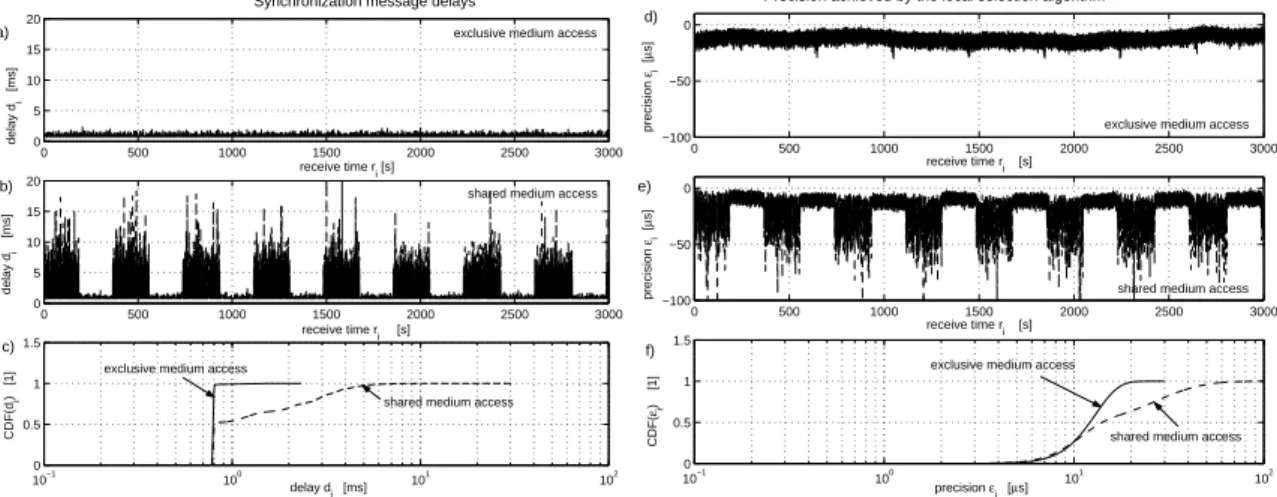
We recorded two streams of 150’000 synchronization messages each, received in ca. 50 minutes, i.e. on average one synchronization message is received every 20 ms. The first scenario is that of a completely empty communication medium. In the second scenario, the medium is shared with two additional stations that do not participate in clock synchroniza-tion, but periodically exchange large files via ftp. The recorded delays are shown in fig.1, left side.
The deterministic delay of the synchronization messages has been removed a-priori, because it is not subject of this study. Computation time of the algorithm is neglected. The numerical results of the local selection algorithm without drift compensation is shown in fig.1, right side.
0 500 1000 1500 2000 2500 3000 0 5 10 15 20 receive time ri [s] 0 500 1000 1500 2000 2500 3000 0 5 10 15 20 receive time ri [s] delay d i [ms] 10−1 100 101 102 0 0.5 1 1.5 delay di [ms] CDF(d i ) [1]
Synchronization message delays
exclusive medium access
shared medium access
shared medium access exclusive medium access
a) b) c) delay d i [ms] 0 500 1000 1500 2000 2500 3000 −100 −50 0 receive time ri [s] precision εi [ µ s] 0 500 1000 1500 2000 2500 3000 −100 −50 0 receive time ri [s] precision εi [ µ s] 10−1 100 101 102 0 0.5 1 1.5 precision εi [µs] CDF( εi ) [1]
Precision achieved by the local selection algorithm
exclusive medium access
shared medium access
shared medium access exclusive medium access
d)
e)
f)
Fig. 1.Left: Delay of messages in a 802.11b ad-hoc network. a) Exclusive access to the medium, no other stations. b) Medium shared with 2 additional stations that periodically exchange large files via ftp. c) Cumulative probability density function of a) and b). The average delay is different, the minimal delay remains constant.Right:Precision of the local selection algorithmwithout drift compensation. d) Exclusive medium access. e) Shared medium. f) The algorithm achieves in 90% of the time a precision better than 15µs in exclusive medium access scenario and 40µs in the shared medium scenario
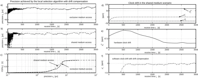
In the implementation of the local selection algorithm with drift compensation, equation (9) has been simplified to βi := max{βi−1 −1/2δhmax(hi −hi−1), βi,i−500}, which reduces
computation time (onlyβi,i−500 has to be evaluated) and memory requirements (500 times
the space required to storecj, hj, βj). The parameterbhas been set to 40µs. Fig.2, left side,
shows the numerical results. Drift compensation improves the achieved precision, especially in the shared medium scenario. Fig.2, right side, shows hardware and software clock drift. Drift compensation removes unknown and variable hardware clock drift.
6 Conclusion
We found algorithms that never actively degrade precision and do not miss to improve precision if there is a chance to do so. The performance in terms of achieved precision these algorithms achieve always improves, if additional synchronization messages are received. This is not the case for probabilistic algorithms [3, 1, 9] and [2]. While the safety property also applies to Lamport’s algorithm [8], only the local selection algorithms are optimal selective.
Experimental results show that the local selection algorithm with drift compensation can achieve synchronization of the non-deterministic delay in the range of 10µs on a standard wireless LAN in ad-hoc mode requiring less than one received synchronization message every 20ms. These parameters match with the requirements of high-quality audio distribution and the capabilities of commonly available technology (wireless LAN, Linux PCs). The results are comparable to those of [5]. While our algorithm seems to require more communication, it can also be used when no broadcast medium is available.
Schreiber and Sigg describe in their master thesis [14] an implementation of the local selection algorithms on Linux PCs that achieves a precision of 40µs. The discrepancy to the 10µs achieved in simulation is mainly due to the simple deterministic delay elimination mechanism used.
Deterministic delay elimination is not possible without communication in the inverse direction, i.e. from the consumer to the producer. It is straightforward to combine the local selection algorithms with a mechanism that progressively removes the deterministic delay by exchanging messages with the synchronization source in a client-server style, rather than the producer-consumer pattern employed by the local selection algorithms. It remains to
0 500 1000 1500 2000 2500 3000 −40 −20 0 receive time ri [s] precision εi [ µ s] 0 500 1000 1500 2000 2500 3000 −40 −20 0 receive time ri [s] precision εi [ µ s] 10−1 100 101 102 0 0.5 1 1.5 precision εi [µs] CDF( εi ) [1]
Precision achieved by the local selection algorithm with drift compensation
exclusive medium access
exclusive medium access shared medium access
shared medium access
a) b) c) 0 500 1000 1500 2000 2500 3000 −50 0 50 100 receive time ri [s] [ppm] 0 500 1000 1500 2000 2500 3000 67 67.5 68 receive time ri [s] ρ h [ppm]i 0 500 1000 1500 2000 2500 3000 −0.5 0 0.5 receive time ri [s] ρ ’i [ppm]
Clock drift in the shared medium scenario
ρh i
ρ’
i
ρi
hardware clock drift
software clock drift with drift compensation
d)
e)
f)
Fig. 2.Left:Precision of the local selection algorithmwithdrift compensation. a) Exclusive medium access. b) Shared medium. c) The algorithm achieves in 90% of the time a precision better than 8µs in both scenarios.
Right:Drift rate of the hardware clock and the two synchronized clocks, all for the shared medium scenario.
d) The drift of the software clock without drift compensation ρ(t) is equal to the hardware clock drift
ρh(t) minus the maximal hardware clock driftρhmax = 100ppm. The drift of the software clockwith drift compensation ρ0(t) is initially equal to that of the software clock without drift compensation and strives
towards zero. e) Close-up ofρh(t). f) Close-up ofρ0(t), considerably more stable thanρh(t).
be studied, how this combination can be made most efficient in terms of total bandwidth consumption and local memory and computation requirements.
References
1. Gianluigi Alari and Augusto Ciuffoletti. Implementing a probabilistic clock synchronization algorithm.
Real Time Systems, 13(1):25–46, 1997.
2. K. Arvind. Probabilistic clock synchronization in distributed systems. IEEE Transactions on Parallel
and Distributed Systems, 5(5):474–487, May 1994.
3. Flaviu Cristian. Probabilistic clock synchronization.Journal of Distributed Computing, 3:146–158, 1989. 4. Danny Dolev, R¨udiger Reischuk, Ray Strong, and Ed Wimmers. A decentralized high performance time service architecture. Technical Report 95/26, Institute for Computer Science, University of L¨ubeck, November 1995.
5. Jeremy Elson, Lewis Girod, and Deborah Estrin. Fine grained network time synchronization using reference broadcasts. Technical Report 020008, Laboratory for Embedded Collaborative Systems LECS, UCLA, May 2002.
6. Lewis Girod, Vladimir Bychkovskiy, Jeremy Elson, and Deborah Estrin. Locating tiny sensors in time and space: A case study. InInternational Conference on Computer Design ICCD, September 2002. 7. Joseph Y. Halpern, Nimrod Megiddo, and Ashfaq A. Munshi. Optimal precision in the presence of
uncertainty. Journal of Complexity, 1(2):170–196, 1985.
8. Leslie Lamport. Time, clocks and the ordering of events in a distributed system. Communications of
the ACM, 21(7):558–565, July 1978.
9. Cheng Liao, Margaret Martonosi, and Douglas W. Clark. Experience with an adaptive globally-synchronizing clock algorithm. In ACM Symposium on Parallel Algorithms and Architectures, pages 106–114, 1999.
10. Jennifer Lundelius and Nancy Lynch. An upper and lower bound for clock synchronization.Information
and Control, 62(2/3):190–204, August/September 1984.
11. Rafail Ostrovsky and Boaz Patt-Shamir. Optimal and efficient clock synchronization under drifting clocks. InSymposium on Principles of Distributed Computing, pages 3–12, 1999.
12. Boaz Patt-Shamir and Sergio Rajsbaum. A theory of clock synchronization. InProceeding of the 26th
Annual ACM Symposium on Theory of Computing, Montreal , Canada, pages 810–819, May 1994.
13. F. Schmuck and F. Cristian. Continuous clock amortization need not affect the precision of a clock synchronization algorithm. InProceedings of the Nineth ACM Symposion on Principles of Distributed
Computing, pages 133–143, 1990.
14. Eric Schreiber and Daniel Sigg. Clock synchronization for wireless LAN. Master’s thesis, ETH Z¨urich, Departement of Information Technology and Electrical Engineering, Institute TIK, Gloriastrasse 35, ETH Zentrum, 8092 Z¨urich, July 2002. (www.tik.ee.ethz.ch/˜blum).