DMLA: A Dynamic Model-Based Lambda Architecture for Learning and Recognition of Features in Big Data

DMLA: A DYNAMIC MODEL-BASED LAMBDA ARCHITECTURE FOR LEARNING AND RECOGNITION OF FEATURES IN BIG DATA

A THESIS IN Computer Science

Presented to the Faculty of the University Of Missouri-Kansas City in partial fulfillment

Of the requirements for the degree MASTER OF SCIENCE

By

RAVI KIRAN YADAVALLI

B.Tech, Jawaharlal Nehru Technological University – Hyderabad, India, 2013

Kansas City, Missouri 2016

©2016

RAVI KIRAN YADAVALLI ALL RIGHTS RESERVED

iii

DMLA: A DYNAMIC MODEL-BASED LAMBDA ARCHITECTURE FOR LEARNING AND RECOGNITION OF FEATURES IN BIG DATA

Ravi Kiran Yadavalli, Candidate for the Master of Science Degree University of Missouri-Kansas City, 2016

ABSTRACT

Real-time event modeling and recognition is one of the major research areas that is yet to reach its fullest potential. In the exploration of a system to fit in the tremendous challenges posed by data growth, several big data ecosystems have evolved. Big Data Ecosystems are currently dealing with various architectural models, each one aimed to solve a real-time problem with ease. There is an increasing demand for building a dynamic architecture using the powers of real-time and computational intelligence under a single workflow to effectively handle fast-changing business environments. To the best of our knowledge, there is no attempt at supporting a distributed machine-learning paradigm by separating learning and recognition tasks using Big Data Ecosystems.

The focus of our study is to design a distributed machine learning model by evaluating the various machine-learning algorithms for event detection learning and predictive analysis with different features in audio domains. We propose an integrated architectural model, called DMLA, to handle real-time problems that can enhance the richness in the information level and at the same time reduce the overhead of dealing with diverse architectural constraints. The DMLA architecture is the variant of a Lambda Architecture that combines the power of Apache Spark, Apache Storm (Heron), and Apache Kafka to handle massive amounts of data using both streaming and batch processing techniques. The primary dimension of this study is to

iv

demonstrate how DMLA recognizes real-time, real-world events (e.g., fire alarm alerts, babies needing immediate attention, etc.) that would require a quick response by the users. Detection of contextual information and utilizing the appropriate model dynamically has been distributed among the components of the DMLA architecture. In the DMLA framework, a dynamic predictive model, learned from the training data in Spark, is loaded from the context information into a Storm topology to recognize/predict the possible events. The event-based context aware solution was designed for real-time, real-world events. The Spark based learning had the highest accuracy of over 80% among several machine-learning models and the Storm topology model achieved a recognition rate of 75% in the best performance. We verify the effectiveness of the proposed architecture is effective in real-time event-based recognition in audio domains.

v

APPROVAL PAGE

The faculty listed below, appointed by the Dean of the School of Computing and Engineering, have examined a thesis titled “DMLA: A Dynamic Model-based Lambda Architecture for Learning and Recognition of Features in Big Data” presented by Ravi Kiran Yadavalli, candidate for the Master of Science degree, and certify that in their opinion, it is worthy of acceptance.

Supervisory Committee

Yugyung Lee, Ph.D., Committee Chair School of Computing and Engineering

Yongjie Zheng, Ph.D.

School of Computing and Engineering

Sejun Song, Ph.D.

vi TABLE OF CONTENTS ABSTRACT ... iii ILLUSTRATIONS………...vii TABLES ... x 1. INTRODUCTION ... 1 1.1 Motivation ... 1 1.2 Problem Statement ... 2 1.3 Proposed Solution ... 2

2. BACKGROUND AND RELATED WORK... 4

2.1 Terminology ... 4

2.2 Related Work ... 6

2.2.1 Big Data Streaming Tools and Frameworks ... 6

2.2.2 Evaluation on Current Stream Processing Frameworks ... 11

3. PROPOSED FRAMEWORK ... 18

3.1 Overview ... 18

3.2 Dynamic Recognition ... 20

3.3 Feature Extraction Flow... 21

3.4 Apache Spark Workflow ... 22

3.5 Apache Storm Workflow ... 24

3.6 Apache Kafka and REST API ... 28

3.7 Features on JAudio ... 29

3.8 Context Aware Model... 32

3.8.1 Home Context ... 33

3.8.2 Classroom Context ... 34

3.8.3 Outdoor Context ... 36

vii

3.8.5 Contextual features ... 38

4. RESULTS AND EVALUATION ... 43

4.1 Apache Spark ... 43

4.1.1 Machine Learning Algorithms ... 43

4.2 Evaluation ... 53

4.2.1 Feature Based Analysis ... 53

4.2.2 Audio File VS Feature Data ... 54

5. CONCLUSION AND FUTURE WORK ... 56

5.1 Conclusion ... 56

5.2 Limitations ... 56

5.3 Future Scope ... 56

REFERENCES ... 57

viii

ILLUSTRATIONS

Figure Page

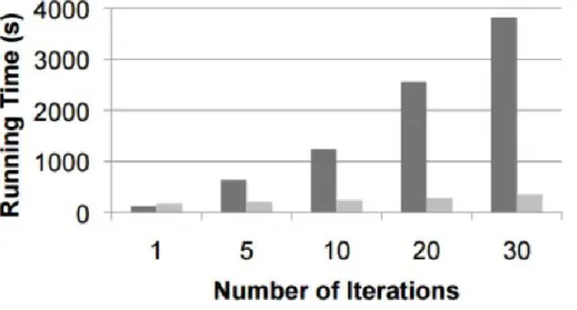
Figure 1: Hadoop vs Spark Runtime Performance ... 9

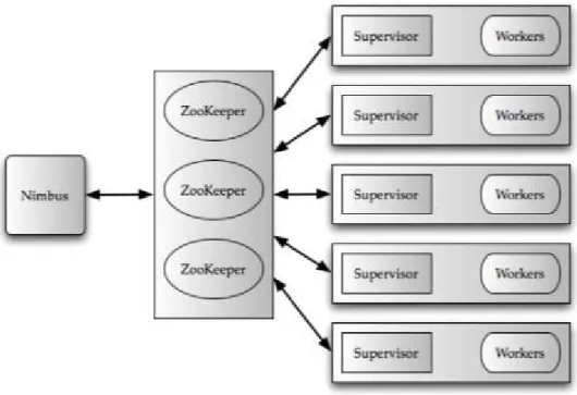
Figure 2: Storm Topology Architecture ... 10

Figure 3: Streaming Applications Workflow ... 12

Figure 4: Lambda Architecture ... 18

Figure 5: Stream Processing Framework Sequence Diagram ... 19

Figure 6: Complete Recognition Model ... 20

Figure 7: Feature Extraction Complete Flow ... 22

Figure 8: Spark Model Building Architecture ... 22

Figure 9: Decision Tree Model ... 23

Figure 10: Storm Topology Recognition ... 25

Figure 11: Storm Topology Visualization ... 25

Figure 12: Single Bolt Topology ... 26

Figure 13: Multiple Bolt Topology ... 27

Figure 14: Hierarchical Bolt Topology ... 28

Figure 15: Kafka Cluster ... 29

Figure 16: Accuracy of Contexts ... 31

Figure 17: Accuracy of Features ... 31

Figure 18: Runtime Performance of Features ... 32

Figure 19: Home Context ... 33

Figure 20: Home Context Wave Form Visualization ... 34

ix

Figure 22: Classroom Context Wave Form Visualization... 35

Figure 23: Outdoor Context ... 36

Figure 24: Outdoor Context Wave Form Visualization ... 37

Figure 25: Office Context ... 37

Figure 26: Office Context Wave Form Visualization ... 38

Figure 27:Rankingof Features ... 43

Figure 28: Spark learning vs Features... 44

Figure 29: Learning in Spark: Static vs Dynamic Data ... 46

Figure 30: Learning in Spark: Static vs Dynamic Data ... 47

Figure 31: Decision Tree Model Evaluation ... 48

Figure 32: Storm ML Model Recognition vs Number of Features ... 49

Figure 33: Storm Recognition vs Classes ... 50

Figure 34: Storm Recognition vs Topologies ... 51

Figure 35: Storm Recognition vs Mobile Recognition ... 52

x

TABLES

Table Page

Table 1: Kafka vs Rabbit MQ Performance ... 14

Table 2: Graph Processing Performance ... 15

Table 3: Communications Flow Comparison ... 16

Table 4: Processing Guarantee Comparison ... 17

Table 5: Home Sample Features ... 39

Table 6: Classroom Sample Features ... 40

Table 7: Outdoor Sample Features ... 41

Table 8: Office Sample Features ... 42

Table 9: Real Time Training Data Performance ... 54

1 CHAPTER 1 INTRODUCTION

1.1

Motivation

Real-time event detection involves the identification of newsworthy happenings (events) as they occur. These events can be mainstream activities, e.g. when a plane crashes into the Hudson River, or local events, e.g. a house fire nearby. Automatic online event detection systems use live document streams to detect events. For instance, streams of newswire articles from multiple newswire providers have previously been used for event detection [1]. Big Data is one of the most popular terms nowadays, but Big Data is not only about the volume. Much of the data is received in real time and is most valuable at the time of arrival.

Around the world, we have 360 million people who have a challenge in hearing [2]. Disabling hearing loss refers to hearing loss greater than 40 dB in the better hearing in adults and greater than 30 dB in the better hearing in children [2]. This thesis discusses one solution to solve the problem of hearing disabled people. The audio analysis and prediction are performed using the big data machine learning platform in apache spark for batch processing and apache storm for real-time audio recognition. Our motivation was to devise a dynamic model which can be available to the hearing challenged pupil at optimal resources.

The inception of the model for this project was from the idea of hearing dog. A hearing dog is a specially trained dog that is owned by people having hearing trouble. The dog hears for any audio sound and then notifies its owner if the audio event is of prominence such as doorbell etc. Also, the other idea was to harness the power of the big data platform and streaming audio data for audio analysis. This is one area that has been unexplored. These simple ideas were the motivation for our study where the primary goal was to develop an audio detection, analysis, and prediction system.

2

1.2 Problem Statement

The unusual growth of data in the recent past has pushed the world into a room of bigger challenges. The synthesis and the processing of this tremendous data to valuable information are the most popular challenge of technology world today. In the exploration of a system to fit in the tremendous challenges posed by the data growth, several ecosystems have evolved; one such is Big Data Ecosystem. Big Data Ecosystem is currently carrying varying architectural models, each one aimed to solve a real-time problem with ease. The problem statement here is to develop a new integrated architecture for audio classification training model and dynamic audio recognition based on the trained model. The each audio model built must be context aware and should have the ability to predict the correct class with in the appropriate context. One have to figure out the most accurate or suitable machine learning model for each of the context through observations and experiments. A dynamic topology has to be generated for identification of each of the class and recognize the audio of variable frame length to predict the audio stream’s category.

1.3 Proposed Solution

This thesis focuses on design of a distributed integrated architectural model for both batch and streaming data. The philosophy of having integrated architectural models to face a superset of real-time problem statements is novel one, which could enhance the richness in information level and at the same time reduce the overhead of dealing with inhomogeneous architectural constraints.

The proposed solution is a Lambda Architecture. Lambda Architecture is a data processing architectural design to handle massive amounts of data using both the streaming and batch processing techniques. The likes of Lambda architecture’s popularity can be directly proportion to the increasing success of big-data, Hadoop and stream processing.

The focus of our study is to design a distributed machine learning model by evaluating the various machine-learning algorithms for event detection learning and predictive analysis with

3

different features in audio domains. We propose an integrated architectural model, called DMLA, to handle real-time problems that can enhance the richness in the information level and at the same time reduce the overhead of dealing with diverse architectural constraints.

4 CHAPTER 2

BACKGROUND AND RELATED WORK

2.1 Terminology

 Decision trees and their ensembles are popular methods for the machine learning tasks of classification and regression. Decision trees are widely used since they are easy to interpret, handle categorical features, extend to the multiclass classification setting, do not require feature scaling, and are able to capture non-linearities and feature interactions. Tree ensemble algorithms such as random forests and boosting are among the top performers for classification and regression tasks [4].

 Naive Bayes is a simple multiclass classification algorithm with the assumption of independence between every pair of features. Naive Bayes can be trained very efficiently. Within a single pass to the training data, it computes the conditional probability distribution of each feature given label, and then it applies Bayes’ theorem to compute the conditional probability distribution of label given an observation and use it for prediction [5].

 Random forests are ensembles of decision trees. Random forests combine many decision trees in order to reduce the risk of overfitting. The spark.ml implementation supports random forests for binary and multiclass classification and for regression, using both continuous and categorical features [6].

 Storm Topology is where; the logic of a real-time application is packaged. It is analogous to map-reduce job. One of the prime differences is that map-reduce job eventually finishes, whereas a topology runs forever. It is a graph of spouts and bolts that are connected with streaming groups.

 Stream is the core abstraction in storm which is unbounded sequence of tuples that is processed and created in parallel in a distributed way. It is defined with a schema that names the

5

fields in the stream’s tuples. It can, by default, contain integers, longs, byte arrays, etc. One can also define their own serializers so that custom types can be used within the topology.

 Spout is a source of streams in a topology. Usually spouts will read tuples from an external source and emit them into the topology.

 Bolts can do anything from filtering functions to aggregations, talking to Databases and more. They can do simple stream transformations and can also do complex transformations using multiple bolts and multiple steps.

 Tasks pertain to one thread of execution and stream groupings define the procedure to send data from one task to another.

 Feature Vector is an n-dimensional vector of numerical features that represent some object. Many algorithms in machine learning require a numerical representation of objects. Since, such representations facilitate processing and statistical analysis.

 Machine learning Model can be either based on supervised learning or unsupervised learning. It is the stored form of the model yielded from the training data passed.

 Events in the audio domain will be the different sounds which can be distinguished uniquely and grouped under a context. Here on, the events are synonymous to the audio classes in each of the environment.

6

2.2 Related Work

2.2.1 Big Data Streaming Tools and Frameworks

Big data is a process of dealing with huge volume, high velocity of heterogeneous data [3]. This kind of data cannot be handled using the traditional data management techniques. Big data tools are the set of tools and techniques that provide the features to store and process the big data efficiently. These tools provide analytical capabilities that help in knowledge mining and decision making process. Apache Hadoop, Apache Spark, Kafka, Tableau etc. are some of the popular big data tools. In this approach use Apache Spark for the processing of audio data.

MapReduce is successful in implementing data intensive applications on commodity clusters but they make use of acyclic flows to execute data flow and this is not useful for certain type of applications which involve using working sets like iterative algorithms [8]. Spark is intended for these type of applications as well and it uses a data abstraction called RDDs (Resilient distributed datasets) to achieve these goals and for fault tolerance. In the storm, the real time stream processing is done and it is fault tolerant. The complex computations in twitter at Scala can be processed in real time by storm. This work gives a brief description on the architecture of Storm and methods to implement fault tolerance and distributed scale-out. This work also illustrates how to execute queries in storm and how flexible it is while dealing with machine failures.

Now-a-days stream processing has become a serious issue of the data pipeline for consumer internet companies. Kafka is introduced as a distributed message system that is developed for collection and delivery of high volumesof data with low latency. Kafka supports both online and offline messaging system. To make Kafka more efficient, few unconventional design choices are made. Experimental results clearly say that Kafka has high performance when compared to other two

7

Stream analysis research has been extensively increased these days, especially on feature extraction and context summary. Deep intelligence framework which is used to reveal the knowledge that is hidden in the stream data. This combines stream processing, batch processing and deep learning in order to realize deep intelligence. This helps in processing the content online. Streaming content consumption has become more popular these days. This has reshaped the internet traffic which made people move from scheduled television to content on demand services. Since the broadcasting services are online, customers are expecting a good bit rates. Wise Replica, which is adaptive replication scheme for peer assisted content on demand systems which will enforce the average bit rate for the Internet content. With the help of the machine learning algorithm, Wise replica will save storage and bandwidth from majority of non-popular contents. Resilient Distributed Datasets (RDDs): It is an immutable i.e. read only collections of objects that are partitioned across cluster. RDD is immutable so, MapReduce algorithms can be applied on them. They can be cached on memory so, they perform better than Hadoop. RDD need not be stored or replicated to achieve fault tolerance but a handle to operations performed on original data is stored so that lost partitions can be rebuilt again parallel. RDDs are default lazy so computationally efficient. Several parallel operations like reduce, collect, map and for-each, filter etc. can be applied on RDD’s. And all programming statements should be deterministic. Spark provides two kinds of shared variables, broad cast variables and accumulators. Broad cast variables send small amount to all nodes. Accumulator variables are used for add only associative operations in driver like count operations in MapReduce [9].

8

Spark is built on top of Mesos, a cluster resource manager. This helps spark to work with existing cluster computing frameworks like Hadoop, HDFS, etc. Any RDD implements three simple operations as an interface,

1. getPartitions, which returns a list of partition IDs. 2. getIterator(partition), which repeats over a partition.

3. getPreferredLocations(partition), this is used for task scheduling in order to achieve data locality.

Apache Spark system is divided in multiple layers, each layer has some responsibilities. The layers work independent of each other.

Interpreter is the first layer and Spark uses a Scala interpreter. As the code is entered in spark console Spark creates an operator graph. When the code runs an action (like collect), the Graph is submitted to a DAG Scheduler. It changes the operators into “stages of different tasks”. A stage can be seta as a set of tasks based on input RDD and number of partitions. The DAG scheduler pipelines all the operators together. Many map operators can be scheduled in a single stage is possible. The final output from a DAG scheduler is a set of stages. So many things can be performed by dividing tasks into map and reduce stages. The Stages are passed on to the Task Scheduler. The task scheduler will launch tasks via cluster manager - Spark Standalone/Yarn/Mesos. The task scheduler doesn't know about dependencies between stages. The Worker executes the tasks on the Slave machine or node. A new JVM is started for a JOB. The worker knows about the code that is assigned to it by task

scheduler. The shared variables are implemented using their custom serialization formats.

Spark mainly uses Scala interpreter but Spark is also available in java, python. They made two changes to actual Scala interpreter to make it work with Spark. The interpreter will output classes to a shared filesystem from which custom java class loaders can be used. To propagate the updates made

9

by singleton objects to workers, they changed the generating code to reference previous line as well in the code.

For the evaluation, spark is used for logistic regression, alternating least squares, and dumping memory access to test for instructiveness of spark.

10

The storm architecture involves processing of streams of tuples flowing through the

topologies. In the topology we have vertices and edges. The Vertices represent computations and the edges describe the flow of data between the computational components. Vertices are further

classified into two different sets namely Spouts and Bolts. The data from the queries Such as Kafka is pulled by the spouts. The incoming tuples are processed by the bolts and passes them to next stream of bolts. Storm topology involves cycles. Storm is generally processed on a distributed cluster and twitter on mesos. In the figure, the Nimbus is the master node and is responsible for assigning and correlate the execution of topology. The worker nodes process the actual work to be done.

11

The worker node runs on one or more worker process. More than one worker process is involved at any point of time during execution and this worker process is to be mapped to a single topology on the cluster. One or more worker processes from the same machine may involve

executing different parts of the same topology. This worker process is executed on the JVM. Through this process parallelism has been provided by the tasks. Each spout or a bolt consists of set of tasks running on the same machine. Storm has five different partitioning strategies. They are:

1. Shuffle grouping: The tuples are grouped randomly. 2. Field grouping: The subset of the tuple field is hashed.

3. All grouping: The complete stream of data is replicated over the consumer tasks. 4. Global grouping: The total stream of data is sent to a single bolt for processing. 5. Local grouping: The tuples are sent to the consumer bolts through the same executer.

2.2.2 Evaluation on Current Stream Processing Frameworks

environments are pushed to servers for real time processing. These applications include sensor-based monitoring, stock trading, web traffic processing, network monitoring, and mobile devices [10]. The data generated by these applications can be seen as streams of events or tuples. In stream-based applications this data is pushed to the system as unbounded sequences of event tuples. Since

immense volumes of data are coming to these systems, the information can no longer be processed in real time by the traditional centralized solutions. A new class of systems called distributed stream processing frameworks (DSPF) has emerged to facilitate such large-scale real time data analytics.

There are many frameworks developed to deploy, execute and manage event-based applications at large scale, and this is one important class of streaming software. Examples of early event stream processing frameworks included Aurora, Borealis, StreamIt and SPADE. With the emergence of Internet-scale applications in recent years, new distributed map-streaming processing

12

models have been developed such as Apache S4, Apache Storm, Apache Samza, Spark Streaming, Twitter’s Heron and Neptune, with commercial solutions including Google Millwheel, Azure Stream Analytics and Amazon Kinesis. Apache S4 is no longer being developed actively. Apache Storm shares numerous similarities with Google Millwheel, and Heron is an improved implementation of Apache Storm to address some of its execution inefficiencies.

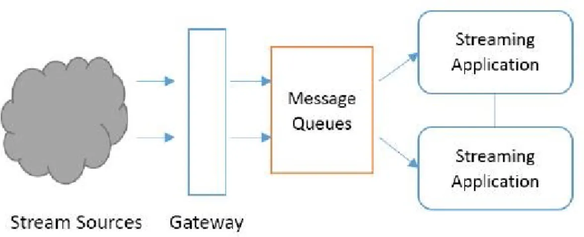
Figure 3: Streaming Applications Workflow

We can evaluate a streaming system on two largely independent dimensions. In one dimension there is a programming API for developing the streaming applications, and the other has an execution engine that executes the streaming application. In theory a carefully designed API can be plugged into any execution engine. A subset of modern event processing engines were selected in this paper to represent the different approaches that DPSFs have taken in both dimensions of

functionality, including a DSPF developed in academia i.e. Neptune. The engines we consider are:

1. Apache Storm [13]: Apache Storm is a free and open source distributed real-time computation system.

2. Apache Spark [12]: Apache Spark is a fast and general engine for big data processing, with built-in modules for streaming, SQL, machine learning and graph processing.

13

3. Apache Flink [14]: Apache Flink is an open source platform for distributed stream and batch data processing. Flink’s core is a streaming dataflow engine that provides data distribution,

communication, and fault tolerance for distributed computations over data streams.

4. Apache Samza [15]: Apache Samza is a distributed stream processing framework. It uses Apache Kafka for messaging, and Apache Hadoop YARN to provide fault tolerance, processor isolation, security, and resource management.

5. Neptune [10]: A real-time distributed stream processing framework.

We would like to evaluate these five modern distributed stream processing engines to compare the capabilities they offer and their advantages and disadvantages along both dimensions of functionality.

Distributed Stream Processing has a strong connection to message queuing middleware. Message queuing middleware is the layer that compensates for differences between data sources and streaming applications. Message queuing is used in stream processing architectures for two major reasons.

1. It provides a buffer to mitigate the temporal differences between message producing and message consuming rates. When there is a spike in message production, they can be temporally buffered at the message queue until the message rate comes down to normal. Also when there is a slowdown in the message processors, messages can be queued at the broker.

2. Messages are produced by a cloud of clients that makes a connection to the data services hosted in a different place. The clients cannot directly talk to the data processing engines because different clients produce different data and these have to be filtered and directed to the correct services. For such cases brokers can act as message buses to filter the data and direct them to appropriate message processing applications.

14

Table 1: Kafka vs Rabbit MQ Performance

Kafka [16] RabbitMQ [10]

Latency Polling clients and disk-based data

storage makes it less friendly to latency critical applications.

In memory storage for fast transfer of messages.

Throughput Best write throughput with scaling

and multiple client writing to same topic. Multiple clients can read from same topic at different locations of message queue at the same time.

Single client writing to the same topic. Multiple consumers can read from the same topic at the same time.

Scalability Many clients can write to a queue

by adding more partitions. Each partition can have a message producer implying writers equivalent to partitions.

The server doesn’t keep track of the clients, so adding many readers doesn’t affect the performance of the server.

Maintains the client status in memory, so having many clients can reduce its performance.

Fault tolerance Support message replication across multiple nodes

Support message replication across multiple nodes

Complex message routing No Supports up to some level, but not

to the level of a service bus.

The graph is abstracted in different ways in different stream processing engines. Some DSPFs directly allow users to model the streaming application as a graph and manipulate it as such. Others do not allow this function and instead give higher level abstractions which are hard to recognize as a graph but ultimately executed as such. Different DSPFs have adopted different terminologies for the components of the graph.

15

Table 2: Graph Processing Performance

Storm[13] Spark[12] Flink[14] Samza[15] Neptune[10] Graph Node Spout or Bolt An operator on

a RDD

Operator on a DataStream

Task Stream Sources

and Stream Processors

Graph Edge Stream Defined

implicitly by the operators on RDDs Defined implicitly by the operators on Data Stream

Kafka Topic Links

Graph is directly created by user

Yes No No Yes Yes

Message abstraction

Tuple RDD Data Stream Envelope Stream Packet

Primary operator implementatio n language

Java Java/Scala Java/Scala Java Java

Name of Graph Topology Stream processing job

Stream Processing job

Samza Job Stream Processing Graph Communications involve serializing the objects created in the program to a binary format and sending them over TCP. Different frameworks use different serialization technologies and this can be

customized. The communications can do optimizations such as message batching to improve the throughput sacrificing latency. Usually the communications are peer to peer and the current DSPFs don’t implement advanced communications optimizations. Communications can be either pull based or poll based while pull based providing the best latency. Poll based systems can have the benefit of not taking messages that cannot process at a node.

Flow control is a very important aspect in streaming computations. When a processing node becomes slow the upstream nodes can produce more messages than the slow node can process. This can lead to message build ups in the upstream nodes or message losses at the slow node depending

16

on the implementation. Having flow control can prevent such situations by slowing down the upstream nodes and eventually not taking messages from the message brokers to process.

Table 3: Communications Flow Comparison

Storm[13] Spark [12] Flink [14] Samza [15] Neptune [10] Data serialization Kryo serialization of Java objects RDD serialization Data Stream Serialization Custom serialization Java Objects

Task Scheduler Nimbus, can use resources allocated by Yarn

Mesos, Yarn Job Manager on top of the resources allocated by Yarn and Mesos Yarn Granules Communicatio n framework

Netty Netty Netty Kafka Netty

Message Batching for High

throughput

Yes Yes Yes Yes Yes

Flow control No Yes Yes Yes Yes

Message delivery

Pull Pull Pull Poll Pull

There are several methods of achieving processing guarantees in streaming environments. The more traditional approaches are to use active backup nodes, passive backup nodes, upstream backup or amnesia. Amnesia provides gap recovery with the least overhead. The other three approaches can be used to offer both precise recovery and rollback recovery. All these methods assume that there are parallel nodes running in the system and these can take over the responsibility of a failed task.

Before providing message processing guarantees, systems should be able to recover from faults. If a system cannot recover automatically from a fault while in operation, it has to be manually maintained in a large cluster environment, which is not a practical approach. Almost all the modern distributed processing systems provide the ability to recover automatically from faults like node

17

failures and network partitions. Now let’s look at how the five frameworks we examine in this paper provide processing guarantees.

Table 4: Processing Guarantee Comparison

Storm [13] Spark [12] Flink [14] Samza [15] Neptune [10] Recover from

faults

Yes Yes Yes Yes No

Message processing guarantee

At least once Exactly once Exactly once At least once Not available

Message guarantee mechanism Upstream backup Write ahead log

Check-pointing Check-pointing Not available

Message guarantee effect on performance

18 CHAPTER 3 PROPOSED FRAMEWORK

3.1 Overview

The demand for stream processing is increasing. Immense amounts of data have to be processed fast from a rapidly growing set of disparate data sources. This pushes the limits of traditional data processing infrastructures. These stream-based applications include trading, social networks, Internet of things, system monitoring, live results tracking and many other real-time system examples. A number of powerful, easy-to-use open source platforms have emerged to address this. But the same problem can be solved differently, various but sometimes overlapping use-cases can be targeted or different vocabularies for similar concepts can be used. This may lead to confusion, longer development time or costly wrong decisions.

Figure 4: Lambda Architecture

 Batch Layer: Unrestrained computation. The batch layer can calculate anything, given enough time

19

 Speed Layer: All the complexity is isolated in the Speed Layer. If anything goes wrong, it’s auto-corrected

 Serving Layer: This layer queries the batch & real-time views and merges it.

Figure 5: Stream Processing Framework Sequence Diagram

We specified three types of events related to task usage that can be reported by a task back to the platform [11]:

 Number and types of recent interactions with an actuator (“recent” is defined by a configurable time window).

20

 Number and types of recent database transactions.

 Probability of topology termination based on the most recent task executions (this metric shows the ratio with which incoming stream items do not lead to any outgoing stream and it can be important when deciding where to execute the tasks).

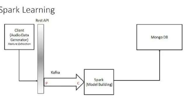
3.2 Dynamic Recognition

Figure 6: Complete Recognition Model

Dynamic Recognition model is the combination of the Batch training and Real-time prediction system. The model has low latency and high performance in clustered environment. Multiple sources through client application can train the data using spark model building techniques. Message broker Kafka helps us achieve high scalability and fault-tolerance from message communication between client and spark. In terms of testing data, a feature vector is sent to storm through Kafka producer by an REST service from client application. Once the data is received to Kafka spout, each of the tuple is sent to several Bolts for processing and synthesis to extract intermediate outputs. The synthesis is

21

based on the decision tree model built on spark. The intermediate outputs can be aggregated using an aggregator bolts. The results from aggregation are stored in mongo DB for visualization.

3.3 Feature Extraction Flow

In this section we would be briefly explaining about the feature extraction flow. A real-time audio is constantly received by the Android client through a listener. Once the audio is received, the Fast Fourier Transformation is applied to the audio input stream and the transformed sound is fed to the JAudio feature extractor in order to extract various features. These features are saved in a text file which will be used as training dataset in Spark for model building.

Once the model is successfully built, the same procedure of collecting features from a real-time audio is applied. The received features are processed with the already built model during model training phase to emit predictions. These predictions are analyzed and the client is notified about the recognition from model prediction phase.

22

Figure 7: Feature Extraction Complete Flow

Figure 7 shows the light weight feature extraction from the client and the distributed computing achieved with Spark for training and testing. The architecture is highly scalable and fault tolerant. The updated model can be saved in Spark in order to predict results for real-time input on the go. The audio data is collected by the mobile device listener and data is converted to a fast fourier transformer wave and features are extracted out of it for learning and recognition.

3.4 Apache Spark Workflow

Figure 8: Spark Model Building Architecture

On the Spark server engine side, before the application actually runs the models are trained using data in the form of .wav files. To improve the accuracy samples of real time data, i.e. data recorded through Android device is also fed into the training data. For training based on the audio files the Spark server uses JAudio library to extract features from the audio files. These files are sampled and features are extracted for each sample. The ratio of samples can be user defined by defining the sample length through the JAudio library.

23

For each context models are trained and saved into the filesystem. Once the data from the client arrives through the socket, the Spark server checks the context information to load the

appropriate model to be used. Then the server uses the feature extraction information to predict the audio class based on the values of the features that were received.

Once the predicted audio class data is ready, it is then sent back to android client using the socket connection. On receiving the predicted audio class the client displays a notification to the user. This notification is intended to alert the user of the audio event that was recorded.

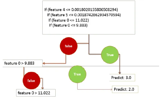
Figure 9: Decision Tree Model

The outcome of spark machine learning model is that a decision tree model like above figure is built which can help us predict the label of the class. Decision Tree is bunch of if-else statements based on feature vector values to identify a leaf-node, which is a class in a context.

24

3.5 Apache Storm Workflow

Storm defines computation in terms of data streams flowing through a graph of connected processing instances. These instances are held in-memory, may be replicated to achieve scale and can be run dynamically on multiple machines. The graph of inter-connected processes is referred to as a topology. A single Storm topology consists of spouts that inject streams of data into the topology and bolts that process and modify the data. Topologies facilitate the modularization of complex processes into multiple spouts and bolts. By connecting multiple spouts and bolts together, tasks can be distributed and scaled

Apache Storm has the following advantages in terms of performance benchmarks.

1. Scalable: The operations team needs to easily add or remove nodes from the Storm cluster without disrupting existing data flows through Storm topologies (aka. standing queries).

2. Resilient: Fault-tolerance is crucial to Storm as it is often deployed on large clusters, and hardware components can fail. The Storm cluster must continue processing existing topologies with a minimal performance impact.

3. Extensible: Storm topologies may call arbitrary external functions (e.g. looking up a MySQL service for the social graph), and thus needs a framework that allows extensibility.

4. Efficient: Since Storm is used in real-time applications; it must have good performance characteristics. Storm uses a number of techniques, including keeping all its storage and computational data structures in memory.

5. Easy to Administer: Since Storm is at that heart of user interactions on Twitter, end-users immediately notice if there are (failure or performance) issues associated with Storm. The operational team needs early warning tools and must be able to quickly point out the source of problems as they arise. Thus, easy-to-use administration tools are not a “nice to have featured,” but a critical part of the requirement.

25

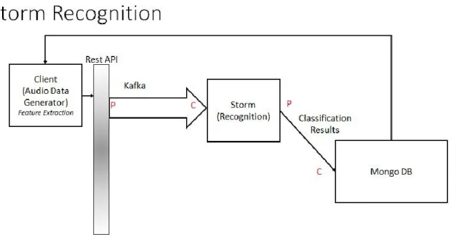
Figure 10: Storm Topology Recognition

Storm can receive the data continuously from Kafka spout and emit the tuples to various processing bolts. Bolts are the processing centers for tuples received through spout and the emitted results can be stored in MongoDB for further evaluation. Tuples are the data objects coupled closely to bolts. Several transformations of tuples are possible in execute method of Bolt.

26

Figure 12: Single Bolt Topology

The complete machine learning model is dynamically loaded into storm from Mongo DB. The Outcome of the Bolt is a Single Decision. The single Recognition Bolt will identify the class the audio belongs to from set of classes.

27

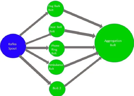
Figure 13: Multiple Bolt Topology

The complete machine learning models is dynamically loaded into storm from Mongo DB and is split to multiple Bolts. The Outcome of the Bolt is an Aggregation from individual Bolts. Each Recognition Bolt would give a Boolean decision for class. The aggregation bolt collects the results from each of the spanning tree bolt.

28

Figure 14: Hierarchical Bolt Topology

The complete machine learning model is dynamically loaded into storm from Mongo DB and is split multi- level bolts. The Outcome of the Bolt is an input to the next level bolt. Each Recognition Bolt would predict a class or level and therefore expects to parse the remaining of the model tree. The aggregation bolt collects the results from each of the final level tree bolt.

3.6 Apache Kafka and REST API

 The Producer API allows an application to publish a stream records to one or more Kafka topics.

 The Consumer API allows an application to subscribe to one or more topics and process the stream of records produced to them.

29

 The Streams API allows an application to act as a stream processor, consuming an input stream from one or more topics and producing an output stream to one or more output topics, effectively transforming the input streams to output streams.

The Connector API allows building and running reusable producers or consumers that connect Kafka topics to existing applications or data systems. For example, a connector to a relational

database might capture every change to a table.

Figure 15: Kafka Cluster

3.7 Features on JAudio

The different features which can be extracted for a input audio stream in JAudio are listed below. In each context scenario, we choose only those features which could best represent the types of classes in a context.

30

1. Peak detection (PD) is the detection of the points in time that a sound signal exceeds a certain threshold.

2. Zero crossing rate (ZCR) is the rate of sign-changes along a signal or the number of times the sound signals cross the x-axis. This feature excels in separating voiced and unvoiced frames. The human voice contains both voiced and unvoiced parts.

3. The Root Mean Square of the waveform calculated in the time domain to indicate its loudness. Corresponds to the ‘Energy’ feature.

4. Fraction of Low Energy Windows is the fraction of the last 100 windows that has an RMS less than the mean RMS in the last 100 windows. This can indicate how much of a signal is quiet relative to the rest of the signal.

5. Spectral Roll-off is the frequency bin below which 93% of the distribution is focused; this is a degree of the skewness of the spectral distribution.

6. MFCCs (Mel Frequency Cepstrum Coefficients) are motivated by the human auditory system. Human sensitivity of frequencies does not follow a linear scale. Variants in lower frequencies are perceived more precisely than variations in high frequencies.

7. Compactness: A degree of the noisiness of a signal. Established by comparing the components of a window's magnitude spectrum with the magnitude spectrum of its adjacent windows.

31

Figure 16: Accuracy of Contexts

The above figure shows the performance of different features pertaining to each of the contexts. For example, it is observed that the accuracy of recognition is high in case of Gender context using the frequency distribution (FD) feature of audio. In general, MFCC happens to perform the best in recognizing the correct class in a given context.

Figure 17: Accuracy of Features

The above figure shows the accuracy achieved per feature vectors of Jaudio on

different contexts and it is observed that Haar and MFCC performing the best for given

contexts. Whereas the highest performing individual feature happens to be the Frequency

32

Figure 18: Runtime Performance of Features

The relative execution times of different features are given in the list and the MFCC happens to have to have highest execution time, yet has very high accuracy. Hence it is always chosen as a key feature despite its high running time.

3.8 Context Aware Model

Context aware systems are a component of ubiquitous computing or pervasive computing environment [7].The goal is to make the mobile computer capable of sensing the users and their current state, exploiting context information to significantly reduce demands on human attention. To minimize user distraction, a pervasive computing system must be context-aware. In our current work, we have devised four important contexts based on the geographical prevalence.

Each of the below discussed context has around 5 classes in each context, which depict the most important activities of the user in the corresponding context .The application is designed in a such a way that the activity/event is recognized based on the current context and alerts the user through a notification on device.

33

3.8.1 Home Context

The Home context would be set to alert the user about the most significant activities when user is around geolocation of home. The purpose of a home context is to identify the key activities of user in day to day life. Once the user identifies the key activities, he can train them as different classes under this context for future recognition.

Figure 19: Home Context

The different classes under home context are

1. Telephone: The Telephone context at home would signify a ringing sound from a home telephone or a cellular device.

2. Door knock: The Door knock context signifies a knock on the door in home environment. 3. Doorbell: The Doorbell scenario will highlight common sounds of a doorbell in home context. 4. Dog bark: The dog bark context can identify with different types of sound from the bark of a dog at home.

5. Siren: The siren context in home context will include emergency alarms such as fire alarms, security threats at home, etc.

34

Figure 20: Home Context Wave Form Visualization

3.8.2 Classroom Context

The Classroom context would be useful in identifying the activities in the classroom of the user. The possible events could be a lecture taking place, an emergency alarm or a discussion in the classroom.

35 The classes under Classroom context are:

1. Siren: The siren context in classroom context will include emergency alarms such as fire alarms, security threats, etc. in school environment.

2. Man: The man context will highlight male voice sounds in a classroom.

3. Woman: The woman context will highlight female voice sounds in a classroom.

4. Group: The group context will highlight more than one female or male voice sounds in a classroom.

36

3.8.3 Outdoor Context

The Outdoor context would be enabled when the user is driving or when the user is exposed to an open-air environment. This would help the user in identifying any alarming activities on the road and alert the user.

Figure 23: Outdoor Context

The classes under Outdoor context are:

1. Ambulance: The Ambulance alarm and siren sounds are identified under this class. 2. Horn: The horn sounds from vehicles are identified under this class.

3. Police: The police vehicle’s siren alerts sounds are identified in this class.

4. Traffic: The traffic class identifies the noises noticed during heavy congestions on road. 5. Train: The different sounds emitted from a train are captured in this class.

6. Vehicle (Car, Motorbike): The vehicle class senses the sounds from different two wheeler and four wheeler vehicles.

37

Figure 24: Outdoor Context Wave Form Visualization

3.8.4 Office Context

The Office context would capture and alert vital events when user is in office. These events could be possibly the sounds of several devices or gadgets which generally used for communication in the office.

38 The classes under Outdoor context are:

1. Desk bell: The desk bell class signifies the sounds from different bells for service in the office environment.

2. Keyboard: The keyboard typing sounds are captured under this class.

3. Fax: Fax alerts and fax machine running sounds in the office are recognized in the fax class. 4. Office door: Office door opening and shutting sounds are captured in the office door class. 5. Phone: The cellular and telephone ringing sounds of the office are recognized in this class. 6. Printer: The printer class identifies various sounds from the office printing machines.

Figure 26: Office Context Wave Form Visualization

3.8.5 Contextual features

The most significant features for home context are Compactness and MFCC. These features can correctly classify the classroom activities to corresponding classes.

The decision tree for this context has a depth of 5 and 21 nodes. The spanning trees could correctly label each of the class from the decision tree model.

39

Table 5 shows the sample features values for different classes in home context. Table 5: Home Sample Features

Class Zero

Cross ing

MFCC Spectral Roll

Off

Peak Value RMS Compactness Fraction of

Low Energy Windows Teleph one 17.19 8 6.4000144900 84054 0.00450390 625 0.04266666666 666665 7.39571384741 4926E-4 0.008650060383 35191 636.1971371 271076 Doork nock 14.85 6 6.4000213476 15432 0.00406738 28125 0.04266666666 666665 2.98472578828 03524E-4 0.007734650891 316967 653.9503031 006038 Doorb ell 8.807 6.4000063181 30669 0.00248779 296875 0.04266666666 666665 4.12487389586 4025E-4 0.003569621600 0250477 683.2859511 11393 Dogbar k 14.10 6 6.4000104810 406855 0.00256542 96875 0.04266666666 666665 1.82076200539 99944E-4 0.004052412511 388329 651.4340836 352274 Siren 22.77 3 6.4000956966 31952 0.00900830 078125 0.04266666666 666665 0.00343367580 9666451 0.056676612669 82051 324.7194988 563841

In table 5, the most significant features for classroom context are Compactness and MFCC. These features can correctly classify the classroom activities to corresponding classes. The decision tree for this context has a depth of 5 and 21 nodes. The spanning trees could correctly label each of the class from the decision tree model. Table 5 shows the sample features values for different classes in office context.

40

Table 6: Classroom Sample Features

ClassRoo m Zero Crossing MFCC Spectral Roll Off

Peak Value RMS Compactness

Fraction of Low Energy Windows Siren 12.081 6.40003 043287 9214 0.0061455 078125 0.04266666666 666665 0.002642619852 6988184 0.020974373548 93187 448.87528089 151414 Man 8.295 6.40000 537807 4125 0.0024746 09375 0.04266666666 666665 1.036937096571 0008E-4 0.001957488770 6529163 678.01187391 24316 Woman 11.852 6.40003 275627 9287 0.0059165 0390625 0.04266666666 666665 8.275344874519 14E-4 0.014278280763 170673 640.69509863 6625 Group 11.433 6.40000 383628 9739 0.0031699 21875 0.04266666666 666665 5.027383033026 648E-5 0.001176044147 0179542 661.11984782 3091

In table 6, the significant features in the home context are RMS and Spectral Roll Off which could correctly classify the events to appropriate classes. This has the decision tree with a depth of 5 and having 33 nodes. The various spanning trees could correctly label each of the class from the decision tree model. Table 6 shows the sample features values for different classes.

41

Table 7: Outdoor Sample Features

Out Door Zero Cross ing MFCC Spectral Roll Off

Peak Value RMS Compactness

Fraction of Low Energy Windows Ambula nce 117.2 1 799.78619825 48343 0.20666666666 666667 150.47721741 661945 0.06939453 125 3932.1387766 719226 32.548268762 45168 Horn 65.55 142.39445117 349476 0.11999999999 999997 14.180537678 19874 0.08183593 75 2224.5983352 975654 18.917546286 145356 Police 122.4 7 162.64174963 18415 0.13999999999 999996 4.5477088441 12729 0.09760253 90625 2357.2694785 83858 22.033538458 42048 Traffic 170.6 4 105.82071270 580484 0.28000000000 000014 16.199522332 341193 0.15255859 375 5134.0673716 78831 43.441276270 69722 Train 120.0 201.30429275 7232 0.16666666666 66666 10.708176546 111845 0.11869140 625 3014.0134634 61915 26.338728397 79567 Vehicle 148.7 1 232.57912378 520254 0.20666666666 666667 8.1358935508 60294 0.09444824 21875 3621.2184729 63309 32.862534136 147254

In table 7, the significant features in the office context are Zero crossing and MFCC which correctly classifies the office events to corresponding classes. The decision tree has a depth of 5 and 38 nodes. The spanning trees could correctly label each of the class from the decision tree model. Table 8 shows the sample features values for different classes in office context.

42

Table 8: Office Sample Features

Office Zero Cross ing MFCC Spectral Roll Off

Peak Value RMS Compactness

Fraction of Low Energy Windows Printer 191.3 325.54124 9784738 0.28000000000 000014 73.597115134 90828 0.21969238 28125 4813.3313780 03683 43.977482471 25381 Office Door 17.07 72.198724 37202147 0.06666666666 666667 11.991216027 091632 0.02067382 8125 1137.4420117 912287 10.559684350 774301 Phone 18.7 69.659608 4943008 0.07333333333 333333 11.468184399 816431 0.03835449 21875 1232.0263855 665005 11.594855330 414326 Fax 93.12 104.54954 70369279 8 0.10666666666 666665 14.938082276 075852 0.05849609 375 1966.8493570 266512 16.876733356 265046 Keyboard 25.86 62.169119 02208157 0.08666666666 666666 15.318767451 079482 0.06132324 21875 1494.6489932 33488 13.582590988 0317 D esk bell 9 .36 1 58.960993 54553522 0.066 6666666666666 7 8.624 715385893023 0. 0291943359 375 1002. 511108828091 10.89 941986626601 4

In table 8, feature extraction from audio plays a key role in identifying the appropriate features for the class recognition in the each context. The features have been classified largely into domains.one being time domain and other is frequency domain.

43 CHAPTER 4

RESULTS AND EVALUATION

4.1

Apache Spark

The Spark engine receives the extracted features from the android device through socket and builds a model from the training data. The training data is the set of features from device which are collected on the go when a sound is heard. Various combinations of training data features have been tested and finally the below seven features were considered to be the top performing audio features both on client and server. Those are Zero crossings, MFCC, SpectralRollOff, Peak Value, RMS,

Compactness and Fraction of Low Energy Windows.

4.1.1

Machine Learning Algorithms

Figure 27:Rankingof Features

In figure 27, we present in more detail how the different features that have performed in the machine learning. MFCC happens to be the best performing feature among the 10 features.

0 10 20 30 40 50 60 70 80 90

Zero crossing rate MFCC Peak Value RMS Compactness Fraction of low energy windows Spectral roll off point Spectral flux Magnitude spectrum Power spectrum 80.3 82.5 63.5 74.5 56.8 56.9 56.9 49.7 51.5 45.3

Accuracy

44

Figure 28: Spark learning vs Features

In figure 28, we present in more detail how the different machine learning algorithms have performed with the change in the number of features. With the increase up to 7 features have increased the accuracy. Decision Tree algorithms with 7 features have performed the best.

The following three algorithms were considered and experimented with various training and testing data sets and their results have been shown in the evaluations. The ideal machine learning algorithm for the problem statement is Decision Tree. As the model accurately evaluates the incoming data and implements the appropriate decisions to predict the class of audio correctly in a context.

Decision trees and their ensembles are popular methods for the machine learning tasks of classification and regression. Decision trees are widely used since they are easy to interpret, handle categorical features, extend to the multiclass classification setting, do not require feature scaling, and are able to capture non-linearities and feature interactions. Tree ensemble algorithms such as random forests and boosting are among the top performers for classification and regression tasks [4].

13.04 27.16 29.9 56.97 73.17 69.19 63.15 80.89 73.98 0 10 20 30 40 50 60 70 80 90 100

1 Audio feature 7 Audio features 10 Audio features

A

cc

u

rac

y

Features

45

Naive Bayes is a simple multiclass classification algorithm with the assumption of independence between every pair of features. Naive Bayes can be trained very efficiently. Within a single pass to the training data, it computes the conditional probability distribution of each feature given label, and then it applies Bayes’ theorem to compute the conditional probability distribution of label given an observation and use it for prediction [5].

Random forests are ensembles of decision trees. Random forests combine many decision trees in order to reduce the risk of overfitting. The spark.ml implementation supports random forests for binary and multiclass classification and for regression, using both continuous and categorical features [6].

Real time dynamic model training by collecting features using Spark MLlib from client side feature set. Multiple models have been built based on several parameters like efficient set of feature set, machine learning model, number of classes. Server client connection has been established through socket connection.

The aim of this exercise was finding the ideal features set for improving the accuracy of the prediction model. In this evaluation the focus was to find a match for the best model in terms of highest accuracy. At the same time varying the features set size to minimize the effort on the model while trying to increase the accuracy. The figures above present the case that based on the comparison for accuracy for Naïve Bayes, Random Forest and Decision Tree algorithms with 1, 7 and 10 features respectively. From the figure it can be deduced that Decision Tree with 7 features (Zero crossings, MFCC, SpectralRollOff, Peak Value, RMS, Compactness, and FrationOfLowEnergyWindows) resulted in the best accuracy. So it was used in the application.

46

Figure 29: Learning in Spark: Static vs Dynamic Data

In figure 29, we present in more detail how the different types of testing data have impacted the accuracy on static and dynamic learning data. Both Training and Testing data from dynamic collection have performed the best.

In this experiment the focus was on the study of the accuracy of the model prediction with only static data in training versus model prediction of model with real time data included in training.  It was clearly evident that with static data in training the accuracy of the model was only 73

percent as audio data varies with a lot of factors such as noise, context etc.

 When real time data was also added for training of the model there was an increase in the accuracy to 83 percent as most of the real time data captured the variance of the audio data in terms of noise and other factors. This is depicted in the figure above.

0 10 20 30 40 50 60 70 80 90 100 Training-Static Training-dynamic 66.81 73.16 27.02 83.59 A cc u rac y Static Testing Dynamic Testing

47

Figure 30: Learning in Spark: Static vs Dynamic Data

In figure 30, accuracy for the contextual models is relatively higher than the non-contextual model. The model prediction is increased by 5% with respect to model which is unaware of context. The outdoor context apparently has individual best accuracy among the classes. Having any

contextual data to existing features would better the performance of recognition for a model. The same has been learnt through our model that by addition of contextual information the recognition accuracy was increased. Among all the contexts outdoor context had highest accuracy as the classes in outdoor context were largely distributed with respect to features. In the classroom context, the classes are closely coupled and overlapping and therefore accuracy was lowest among the other contextual scenarios. 79 79.5 80 80.5 81 81.5 82 82.5 83 83.5 84 84.5

Non Contextual Contextual

80.81 83.59 84.14 81.96 82.31

None

Home

Outdoor

Classroom

Office

48

Figure 31: Decision Tree Model Evaluation

In figure 31, we present in more detail how the different features that have been discussed have performed in the machine learning under different contexts.

 MFCC happens to be the best performing feature among the 10 features.

 Through our experiments it has been learnt the more the number of features better was the accuracy in each of the context individually.

 If the features were increased over seven, the accuracy gradually decreased in each of the context. So the ideal no of features in each of the context were seven.

0 20 ₄₀ 60 80 100 Office Context Class Context Home Context Outdoor Context

Accuracy

49

Figure 32: Storm ML Model Recognition vs Number of Features

In figure 32, we present in more detail how the different Machine Learning Libraries have performed with increasing number of features. Decision Tree with 7 features was performing the ideal. Time Domain Most feature extraction algorithms necessitate a frequency analysis as the primary step. There is conversely a minor group of algorithms that use the signal in its raw form. These time domain features are often used when processing power is an issue. The preprocessing that needs to be done for this type of feature is less than when using frequency domain features. Applications that are deployed on wireless sensor nodes or on wearable devices often employ time domain features to gain knowledge about the environment. For these devices, battery-life is an important issue, so the algorithms that are being used must be computationally inexpensive.

Naives Bayes Decision Tree Random Forest 0 10 20 30 40 50 60 70 80 90 100 1 Feature 7 Features 10 Features 24.35 32.85 23.56 72.42 74.47 71.88 72.08 72.19 _73.12

Accu

racy

Decision Tree Random Forest

50

Figure 33: Storm Recognition vs Classes

In figure 33, we present in more detail how the storm recognition has been impacted with varying features. Here, we present in more detail how the storm recognition has been impacted with varying features. The observation from this experiment was that the accuracy difference with the change in recognition in storm was almost consistent with the results achieved from recognition through spark. Multiple Bolt recognition with 2 classes had highest accuracy. As the number of classes increased, the accuracy gradually decreased on all the bolt models in storm.

84.73 77.45 73.15 64.56 82.64 74.04 71.78 62.81 81.64 72.14 70.67 67.8 60 65 70 75 80 85 90 95 100

2 Classes 5 Classes 7 Classes 10 Classes

Multiple Bolt single Bolt Hierarchial Bolt

51

Figure 34: Storm Recognition vs Topologies

In the Figure 34, we present in more detail how the storm recognition has been impacted with varying features. Single bolt recognition is a single prediction system from the model generated. The highest accuracy was achieved from seven features and multiple recognition bolt model followed by hierarchical bolt model in storm recognition.

In the Figure 35 below, we present in the execution time and accuracy of different models involved in evaluation. The primary goal of the experiment was to distinguish the run-time

performance of distributed recognition model to that of light weight client side model. Through distributed recognition model, we have achieved five percent more accuracy in almost four times less execution time. The least execution time for recognition was using single bolt recognition model of 0.7 seconds. 47.16 58.29 55.09 74.26 75.49 75.17 67.58 69.15 68.72 30 35 40 45 50 55 60 65 70 75 80

1 features 7 features 10 features

Accu

racy

Single Bolt

Multiple Bolts

Hierarchial Bolts

52

Figure 35: Storm Recognition vs Mobile Recognition

Figure 36: Heron vs Storm Performance 82.7 77.2 84.5 75.8 0 10 20 30 40 50 60 70 80 90 100 0 0.2 0.4 0.6 0.8 1 1.2 1.4 1.6 1.8 2 A cc u rac y Execution Time Accuracy Mobile Recognition model

Single level Bolt _Hierarchical

Bolt 17.28 27.22 0 5 10 15 20 25 30

Storm

Heron

Throughput

53

In Figure 36, we present in more detail how the different distributed platforms for large data. Here we compare the apache storm and twitter heron for real time stream framework performance. The above figure is the evaluation of throughput of results generated from bolts. Twitter heron apparently is the replacement for storm with state full architecture. In our experiments twitter heron is 1.6 times faster than apache storm.

4.2

Evaluation

The application had acceptable performance in terms of the run time required for the entire work flow. In terms of the model training and model saving the run time required was 20 minutes and 34 seconds for the non-contextual model. While it around 6 minutes for each of the four contextual models. The runtime for one cycle of audio recording, feature extraction, prediction of audio class and notification to the user was as following.

 Audio recording is 4 seconds

 Feature extraction and audio class detection at server is 3.42 seconds.  Response from server to client and notification to the user is 1.89 seconds.

4.2.1

Feature Based Analysis

The aim of the exercise is comparison of the accuracy for Non contextual model versus the contextual model. In this exercise we had two models, one where there was no context information for the model. There was only a single model with 20 classes and training data for all the 20 classes. On the other hand we had 4 different models each for one of four contexts. Each contextual model had 5 classes each and training data was limited only to these 5 classes for each model. Then we compared the accuracy of non-contextual model vs each of the contextual model. As the following figure depicts the contextual models outperform the non-contextual model as the contextual models each have limited classes to predict which in turn improves accuracy of the model.

54

Static data, here is an audio file in .wav format. The static sounds have been collected from various repositories like findsounds.com based on the context. Audio features are extracted and trained on the spark machine. Real Time data is collected through MediaRecorder listener on device from sounds on YouTube and findsounds.com to extract features at client side and send them to spark for training.

4.2.2

Audio File VS Feature Data

1. Audio file training has more training time by almost 4 times. 2. Feature data training has yielded more accuracy.

3. Client side Audio file testing has yielded low matching and varied results. 4. Feature vector processing on both client and server has optimal performance. 5. Higher the feature vector, higher is the performance.