SFB 649 Discussion Paper 2011-048
S
FB
6
4
9
E
C
O
N
O
M
I
C
R
I
S
K
B
E
R
L
I
N
Large Vector Auto
Regressions
Song Song *
Peter J. Bickel *
* University of California, USA
This research was supported by the Deutsche
Forschungsgemeinschaft through the SFB 649 "Economic Risk". http://sfb649.wiwi.hu-berlin.de
ISSN 1860-5664
SFB 649, Humboldt-Universität zu Berlin Spandauer Straße 1, D-10178 Berlin
Large Vector Auto Regressions
Song Song
∗, Peter J. Bickel
†July 31, 2011
Abstract
One popular approach for nonstructural economic and financial forecasting is to include a large number of economic and financial variables, which has been shown to lead to significant improvements for forecasting, for example, by the dynamic factor models. A challenging issue is to determine which variables and (their) lags are relevant, especially when there is a mixture of serial correlation (temporal dynamics), high dimensional (spatial) dependence structure and moderate sample size (relative to dimensionality and lags). To this end, an integrated solution that addresses these three challenges simultaneously is appealing. We study the large vector auto regressions here with three types of estimates. We treat each variable’s own lags different from other variables’ lags, distinguish various lags over time, and is able to select the variables and lags simultaneously. We first show the consequences of using Lasso type estimate directly for time series without considering the temporal dependence. In contrast, our proposed method can still produce an estimate as efficient as anoracle under such scenarios. The tuning parameters are chosen via a data driven “rolling scheme” method to optimize the forecasting performance. A macroeconomic and financial forecasting problem is considered to illustrate its superiority over existing estimators.
Keywords: Time Series, Vector Auto Regression, Regularization, Lasso, Group Lasso, Oracle estimator
JEL classification: C13, C14, C32, E30, E40, G10
1
Introduction
Macroeconomic forecasting is one of the central tasks in Economics. Broadly speaking, there are two approaches, structural and nonstructural forecasting. Structural forecasting, which aligns itself with
∗University of California, Berkeley. Email: [email protected] †University of California, Berkeley. Email: [email protected]
economic theory, and hence rises and falls with that, recedes following the decline of Keynesian theory. In recent years, new dynamic stochastic general equilibrium theory has been developed, and structural macroeconomic forecasting is poised for resurgence. Nonstructural forecasting, in contrast, attempts to exploit the reduced-form correlations in observed macroeconomic time series, has little reliance on economic theory, has always been working well and continues to be improved. Various univariate and multivariate time series analyzing techniques have been proposed, e.g. the auto regression (AR), moving average (MA), autoregressive moving average (ARMA), generalized autoregressive conditional heteroskedasticity (GARCH), vector auto regression (VAR) models among many others. A very challenging issue for this nonstructural approach is to determine which variables and (their) lags are relevant. If we omit some “important” variables by mistake, it potentially creates an omitted variable bias with adverse consequences for both structural analysis and forecasting. For example, Christiano et al. (1999) points out that the positive reaction of prices in response to a monetary tightening, the so-called price puzzle, is an artefact resulting from the omission of forward-looking variables, such as the commodity price index. Recently, Ba´nbura et al. (2010) shows that, when using the cross-sectional dimension related shrinkage, the forecasting performance of small monetary vector auto regression can be improved by adding additional macroeconomic variables and sectoral information. To illustrate this, we consider an example of interest rate forecasting. Nowadays people primarily use univariate or multivariate time series models, e.g. the Vasicek, CIR, Jump-Diffusion, Regime-Switching, and time-varying coefficients models, all of which are mostly based on the information from the interest rate time series itself. However, in practice, the central bank (Fed) bases their decisions of interest rate adjustment (as a monetary policy instrument) heavily on the national macroeconomic situation by taking many macro and financial measures into account. Bringing in this additional spatial (over the space of variables instead of from a geographic point of view; also used in future for convenience) information will therefore help improve its forecasting performance. Another example about the interactions between macroeconomics and finance comes from modeling credit defaults by also using macroeconomic information, since variation in aggregate default rates over time presumably reflects changes in general economic conditions also. Figlewski et al. (2006) find credit events are significantly affected by macroeconomic factors. Not only macroeconomics could affect finance, finance could also affect macroeconomics. For example, the economic crisis typically starts from the stock market crash. All of these call for an integrated analysis of macroeconomics and finance. Thus recently there has been a growing trend of using large panel macroeconomic and financial time series for forecasting, impulse response study and structural analysis, Forni et al. (2000), Stock and Watson (2002a), Stock and Watson (2002b), also seen at Forni et al. (2005), Stock and Watson (2005b), Giannone et al.
(2005), and Ba´nbura et al. (2010) for latest advancements.
Besides its presence in empirical macroeconomics, high dimensional data, where information often scatters through a large number of interrelated time series, is also attracting increasing attention in many other fields of economics and finance. In neuro-economics and behavioral finance, one uses high dimensional functional magnetic resonance imaging data (fMRI) to analyze the brain’s response to certain risk related stimuli as well as identifying its activation area, Worsley et al. (2002) and Myˇsiˇckov´a et al. (2011). In quantitative finance, one studies the dynamics of the implied volatility surface for risk management, calibration and pricing purposes, Fengler et al. (2007). Other examples and research fields for very large dimensional time series include mortality analysis, Lee and Carter (1992); bond portfolio risk management or derivative pricing, Nelson and Siegel (1987) and Diebold and Li (2006); international economy (many countries); industrial economy (many firms); quantitative finance (many assets) analysis among many others.
On the methodology side, if people still use either low dimensional (multivariate) time series techniques on a few subjectively (or from some background knowledge) selected variables or high dimensional “static” methods which are initially designed for independent data, they might either disregard potentially relevant information (temporal dynamics and spatial dependence) to produce suboptimal forecasts, or bring in additional risk. Examples include the already mentioned prize puzzle and interest rate forecasting problems. The more scattered and dynamic the information is, the severer this loss becomes. This modeling becomes more challenging under the situation that macroeconomic data we typically deal with has only low frequencies, e.g. monthly or yearly. For example, the pop-ularly used dataset introduced by Stock and Watson (2005a) contains 131 monthly macro indicators covering a broad range of categories including income, industrial production, capacity, employment and unemployment, consumer prices, producer prices, wages, housing starts, inventories and orders, stock prices, interest rates for different maturities, exchange rates and money aggregates and so on. The time span is from January 1959 to December 2003 (soT = 540). In summary, we can see that the challenge of modeling high dimensional time series, especially the macroeconomic ones, comes from a mixture of serial correlation (temporal dynamics), high dimensional (spatial) dependence structure and moderate sample size (relative to dimensionality and lags). To this end, an integrated solution addressing these three challenges simultaneously is appealing.
To circumvent this problem, dynamic factor models have been considered to be quite successful recently in the analysis of large panels of time series data, Forni et al. (2000), Stock and Watson (2002a), Stock and Watson (2002b), also seen at Forni et al. (2005), Giannone et al. (2005), Park et al. (2009) and Song et al. (2010) (nonstationary case). They rely on the assumption that the bulk
of dynamics interrelations within a large dataset can be explained and represented by a few common factors (low dimensional time series). Less general models in the literature includestatic factor models proposed by Stock and Watson (2002a), Stock and Watson (2002b) andexact factor model suggested by Sargent and Sims (1977) and Geweke (1977).
Compared with the well studied dynamic factor models through the use of dynamic principal component analysis, the vector auto regressive (VAR) models have several natural advantages. For example, compared with the dynamic factor models’ typical 2-step estimation procedure: dimension reduction first and low dimensional time series modeling, the VAR approach is able to model the high dimensional time series in one step, which may lead to greater efficiency. It also allows variable-to-variable relationship (impulse response) analysis and facilitates corresponding interpretation, which is not feasible in the factor modeling setup since the variables are “represented” by the corresponding factors. Historically, the VAR models are not appropriate for analyzing high dimensional time series because they involve the estimation of too many (J2P, where J is the dimensionality and P is the number of lags) parameters. Thus they are primarily implemented on relatively low dimensional situations, e.g. the Baysian VARs (BVAR) by Doan et al. (1984) or still through the idea of factor modeling, e.g. the factor-augmented VAR (FAVAR) by Bernanke et al. (2005). However, based on recent advances in variable selection, shrinkage and regularization theory from Tibshirani (1996), Zou (2006) and Yuan and Lin (2006), large unrestricted vector auto regression becomes an alternative for the analysis of large dynamic systems. Therefore, the VAR framework can also be applied to empirical problems that require the analysis of more than a handful of time series. Mol et al. (2008) and Ba´nbura et al. (2010) proceed that from the Bayesian point of view. Chudik and Pesaran (2007) consider the case that P = 1 and both J and T are large through some “neighboring” procedure, which can be viewed as a special case of the “segmentized grouping” as we study here (details in Subsection 2.4). In the univariate case (J = 1), Wang et al. (2007) studies the regression coefficient and autoregressive order shrinkage and selection via the lasso whenP is large andT is small (relative toP).
In this article, we will study the large vector auto regressions when J, P → ∞ and T is moderate (relative to J P). Comparing to prior works in (large) vector auto regressions, the novelty of this article lies in the following perspectives. First, from the variable selection and regularization point of view, the theoretical properties of many existing methods have been established under the indepen-dent scenario, which is rarely met in practice and contradicts the original time series setup (if used directly). Disregarding the serial correlation in variable selection and regularization can be dangerous in the sense that various risk bounds in fact depend on the degree of time dependence, as we will
illustrate later. We propose a new methodology to address this serial correlation (time dependence) issue together with high dimensionality and moderate sample size, which enables us to obtain the consistency of variable selection even under the dependent scenario, i.e. to reveal the equilibrium among them. Second, our method is able to do variable selection and lag selection simultaneously. In previous literature, variable selection is usually carried out first, and then the corresponding estimate’s performances w.r.t. different number of lags are compared through some information criteria to select the “optimal” number of lags. By doing so, we neglect the “interaction” between variable selection and lag selection. Additionally, when the number of the lag’s candidates to be searched over is large, it is also computationally inefficient, due to the cost of the repeated variable selection procedures.
Third, we differentiate the variable of interest’s own lags (abbreviated as own lags afterwards) from the ones of other variables (abbreviated as others’ lags afterwards). Their relative weights are also allowed to be varied when predicting different variables, while in other literature, they are assumed to stay the same. This is due to the fact that the dynamic of some variables is driven by itself, while for a different variable, it might be driven by the dynamics of others. When we include a vast number of macroeconomic and financial time series, assuming the same weight seems to be too restrictive.
Fourth, our method is based on a more computationally efficient approach, which mostly uses the existing packages, e.g. the LARS (least angle regression) package, developed by Efron et al. (2004), while most other works in the literature go through the Bayesian approach that requires the choice of priors.
The rest of the article is organized as follows. In the next section, we present the main ingredients of the large vector autoregressive model (Large VAR) together with several corresponding estimation procedures and comparisons among them. The estimates’ properties are presented in Section 3. In Section 4, the method is applied to the motivating macroeconomic forecasting problem, which shows that it outperforms some major existing method. Section 5 contains concluding remarks with discussions about relaxing some assumptions. All technical proofs are sketched in the appendix.
2
The Large VAR Model and Its Estimation
In this section, we introduce the model with three different estimates first, then discuss the data driven choice of hyperparameters to optimize the forecasting performance, provide a numerical algorithm, and finally summarize comparisons among these three estimates.
2.1
The Model
Assume that the high dimensional time series {Ytj}Tt=1,jJ=1 is generated from
Yt> = Yt>−1B1+. . .+Yt>−PBP +Ut> (1) YT> YT>−1 . . . | {z } T×J = YT>−1 YT>−2 . . . YT>−P YT>−2 YT>−3 . . . YT>−1−P . . . . | {z } T×J P B1 B2 . . . | {z } J P×J + UT> UT>−1 . . . | {z } T×J Y = XB+U, (compact form) (2) where • Y = (YT>, . . . , Y1>)> with Yt> = (Yt1, . . . , YtJ);
• X = (XT>, . . . , X1>)> (the lags of Y) with Xt= (Yt>−1, . . . , Yt>−P)
>;
• B1, . . . , BP areJ×J autoregressive matrices, whereP is the number of lags, B = (B1, . . . , BP)>
is the J P ×J matrix containing all coefficients {Bpij}Pp=1,iJ=1J,j=1, and B··j, Bp·j, B·i·, Bpi· is the
jth column of B and Bp,ith row of B and Bp respectively;
• U = (UT>, . . . , U1>)>, whereUt is a J-dimensional noise and independent of Xt.
All Yt, Xt and Ut are assumed to have mean zero. The J ×J covariance matrix of Ut, Cov(Ut), is
assumed to be independent of t. Here we assume Cov(Ut) to be diagonal, say IJ∗J. In our case, it is
justified by the fact that the variables in the panel we will consider for estimation are standardized and demeaned. Similar assumption is also carried out in Mol et al. (2008). The relaxation allowing nonzero off-diagonal entries is discussed in Section 5.
We can see that given large J and P, we have to estimate a total of J2P parameters, which is much larger than the moderate number of observations J T, i.e. J P T. Consequently, ordinary least squares estimation is not feasible. Additionally, due to the structural change points in the macro and financial data (although not explored in this paper), the effective number of observations used for estimation could be much smaller than the original T. Thus we can see that on one hand, we do not want to impose any restrictions on the parameters and attain some general representations; on the other hand, it is known that making the model unnecessarily complex can degrade the efficiency of the resulting parameter estimate and yield less accurate predictions, as well as making interpretation and variable selection difficult. Hence, to avoid over fitting, regularization and variable selection are necessary. In the following, we are going to discuss the estimation procedure with different kinds of
regularization (illustrated in Figure 1). Before moving on, we incorporate the following very mild belief, as also considered in Ba´nbura et al. (2010): the more recent lags should provide more reliable information than the more distant ones, which tries to strike a balance between attaining model simplicity and keeping the historic information.
• • • • • • 0 • 0 0 0 0 • • • • • • • • • 0 • • • • • • • • • • • • • 0 • 0 • • • • • • • • • • • 0 • • • • 0 • • • • • • • • • • • 0 • • • • • • • • • • • 0 • 0 • • • • • • • • • • • • • • • 0 0 0 • • • • • • • • •
Figure 1: Illustration of three different types of estimates.
2.2
Universal Grouping
Without loss of generality, we start from considering one coefficient matrix, say Bp with entries {Bpij,16i, j 6J}. Inspired by Ba´nbura et al. (2010), we note the fact that the dynamic of some
variable is driven by itself, while for a different variable, it might be driven by the dynamics of others. Consequently, we treat the variables’ own lags (diagonal terms of Bp) different from others’
lags (off-diagonal terms of Bp) and impose different regularizations for them. We assume that the
off-diagonal coefficients of Bp are not only sparse, but also have the same sparsity pattern across
different columns, which we call group sparsity. Thus we base our selection solution on group Lasso techniques (Yuan and Lin (2006)) for the off-diagonal terms and Lasso techniques (Tibshirani (1996)) for the diagonal terms here. We use Bpj−j to denote the vector composed of {Bpji}i6=j and W−j to
denote the (J−1)×(J−1) diagonal matrix diag[w1, . . . , wj−1, wj+1, . . . , wJ] wherewi is the positive
real-valued weight associated with the ith variable for 1 6 i 6 J. It is included here primarily for practical implementation since ifwi is chosen as the Std(Yi), it is equivalent (subsection 2.6 for details)
to standardize the predictors so that they all have zero mean and unit variance, Tibshirani (1996), which is also preferable for comparisons to prior works.
Specifically, given the above notations, we use the group Lasso type penaltyPJ
j=1kBpj−jW−jk2and
Lasso type penalty µPJ
j=1wj|Bpjj| to impose regularizations on other regressors’ lags and predicted
variables’ own lags respectively and have the following penalty for the Bp matrix: J X j=1 kBpj−jW−jk2+µ J X j=1 wj|Bpjj|6Cp−α, (3)
with some generic constant C.
• The hyperparameter µ controls the extent to which others’ lags are less (more) “important” than the own lags. When µ is large, the penalty assigned to own lags is larger than to others’ lags. As a result, it is more likely that the off-diagonal entries are shrunk to 0 instead of the diagonal ones, which corresponds to the case that the variable’s dynamic is driven by itself, and vice versa whenµ is small.
• The item p−α reflects different regularization for different lags (over time). It becomes smaller
when p gets larger. This is consistent with the previous belief: the more recent lags should provide more reliable information than the more distant ones. Thus as a result, large amounts of shrinkage are towards the more distant lags, whereas small amounts of shrinkage are towards the more recent ones. The hyperparameter α governs the relative importance of distant lags w.r.t. the more recent ones. Other decreasing functions of p, e.g. f(p) = log(p)−α, f(p) = exp(p)−α could also be used. However, we do not consider a general representation (and use a data driven way to estimatef(1), . . . , f(p), . . . , f(P) correspondingly) to avoid too many tuning parameters, especially when P → ∞.
Since we haveP coefficient matricesB1, . . . , BP, summing (3) up over p(after multiplyingpα on both
sides) yields PP p=1 PJ j=1pαkBpj−jW−jk2 +µ PP p=1 PJ
j=1pαwj|Bpjj| 6 CP. If we couple this to the
quadratic loss {2J(T−P)}−1PT
t=P+1kY
>
t −Xt>Bk22 through Lagrange multipliers, we have equation (4): min B {J(T −P)} −1 T X t=P+1 kYt>−Xt>Bk22+λ XP p=1 J X j=1 pαkBpj−jW−jk2+µ P X p=1 J X j=1 pαwj|Bpjj| γ=λµ = min B {J(T −P)} −1 T X t=P+1 kYt>−Xt>Bk2 2+λ P X p=1 J X j=1 pαkBpj−jW−jk2+γ P X p=1 J X j=1 pαwj|Bpjj|(4)
with hyperparameters λ, γ and α. We call this estimate ˆB the universal grouping estimate. As the number of variables J increases, the autocoefficients should be shrunk more in order to avoid over-fitting, as already discussed by Mol et al. (2008).
Using the group Lasso type regularization for the off-diagonal terms actually poses some strong assumptions on the underlying structure, which is not realistic from an economic point of view.
Remark 2.2.1 First, we just have one hyperparameter µ (µ= γ/λ) to control the relative weights between own lags and others’ lags. This means that the weights between own’s lags and others’ lags are the same across different dimensions which is hardly met in practice. Correspondingly, when we select the “optimal” µ to optimize the forecasting performance, we are actually optimizing the
averaged forecasting performance for allJ variables instead of the variable of particular interest. This might produce suboptimal forecasts. Ba´nbura et al. (2010) considers a special case that own lags are always more “important” than others’ lags, which might be less general than ours. Remark 2.2.2 Second, using the L2 norm kBpj−jW−jk2 might shrink all off-diagonal terms in the same row ({Bpj·}·6=j) to zero simultaneously, which implicitly means that, for the jth corresponding variable,
we assume it is either significant for all the otherJ−1 variables or not for any other J−1 variables at all. This is, again, too strong from an economic point of view.
2.3
No Grouping
To amend the deficiencies of the universal grouping estimate, we estimate the autocoefficient matrix
B column by column instead of all at once. Without loss of generality, we consider the jth column
B··j here. Since B··j is a vector, we can use the Lasso type penalties for both own lags and others’
lags. By following similar ideas and abbreviations in subsection 2.2, we have equation (5) to get ˆB··j:
min B··j (T −P)−1 T X t=P+1 (Ytj−Xt>B··j)2+λj XP p=1 X i6=j pαwi|Bpij|+uj P X p=1 pαwj|Bpjj| γj=λjµj = min B··j (T −P)−1 T X t=P+1 (Ytj−Xt>B··j)2+λj P X p=1 X i6=j pαwi|Bpij|+γj P X p=1 pαwj|Bpjj| (5)
with hyperparameters λj, γj and α. The subindex j is added to λj and γj to emphasize that they
could vary when estimating different B··j’s, 1 6j 6J. We call this estimate ˆB = ( ˆB··1, . . . ,Bˆ··J) the
no grouping estimate.
Remark 2.3.1 Because of different µj’s (µj = γj/λj) for different columns’ estimates ˆB··j, we
allow individualized weights between own lags and others’ lags and could tuneλj’s andγj’s to produce
optimal forecasting performance for each variable of interest, say the jth. Remark 2.3.2 Also for the same reason, we could get rid of the disadvantage that all off-diagonal terms in one row might be shrunk to 0 simultaneously.
For simplicity of notation, we drop the common subindex j and write Ytj = yt, B··j = β, Bpij = ci, i6=j, Bpjj =dp, λj =λ, γj =γ, and (5) becomes: min β QT(β) = minβ (T −P) −1 T X t=P+1 (yt−Xt>β) 2 +λ P X p=1 X i6=j pαwi|ci|+γ P X p=1 pαwp|dp| = min β (T −P) −1 T X t=P+1 (yt−Xt>β) 2+λ i P(J−1) X i=1 |ci|+γp P X p=1 |dp| (6) with λi =λpαwi and γp =γpαwp.
2.4
Segmentized Grouping
Since the large panel of macroeconomic and financial data sets usually have some natural “segment” structure, e.g. multiple interest rate time series w.r.t. different maturities, different number of em-ployees w.r.t. different industrial sectors, different price indices w.r.t. different goods etc, if we take this information into account instead of estimating B either all at once or column by column, we could also do it segment by segment. Without loss of generality, we consider the ith segment B··Ni.
Ni is the index set for the ith segment and Ni = |Ni| denotes the cardinality of the set Ni. Yt>Ni is
the corresponding part ofYt>. We also use WNi to denote the Ni×Ni diagonal matrix with diagonal
entries {wi}i∈Ni and WNi−j to denote the (Ni −1)×(Ni−1) diagonal matrix with diagonal entries
{wi}i∈Ni,i6=j.
Under this situation, we have: own lags, others’ (in the same segment) lags and others’ (outside the segment) lags for the estimation of the ith segment’s corresponding autoregressive coefficientsB··Ni.
Also following similar ideas and abbreviations in subsection 2.2, we have the following estimation equation: minB··Ni{Ni(T −P)} −1PT t=P+1kY > tNi −X > t B··Nik 2 2 +λNi PP p=1 P j /∈Nip αkB pj·WNik2+µ1Ni PP p=1p αw j|Bpjj|+µ2Ni PP p=1 P j∈Nip αkB pj−jWNi−jk2 minB··Ni{Ni(T −P)} −1PT t=P+1kY > tNi −X > t B··Nik 2 2 +λNi PP p=1 P j /∈Nip αkB pj·WNik2+γNi PP p=1p αw j|Bpjj|+ηNi PP p=1 P j∈Nip αkB pj−jWNi−jk2 (7)
with hyperparameters λNi, γNi, ηNi, α, γNi =λNiµ1Ni and ηNi =λNiµ2Ni, i = 1, . . . , I where I is the
overall number of segments. We call this estimate ˆB = ( ˆB··N1, . . . ,Bˆ··NI) thesegmentized grouping
estimate.
Chudik and Pesaran (2007) consider the case P = 1 and T is large (relative to J) through some “neighboring” procedure, which can be viewed as a special case of the “segmentized grouping” we studied here.
2.5
Forecast Evaluation and Choice of Parameters
The three penalization methods discussed above critically depend on penalty parameter selection for their performance in model selection, parameter estimation and prediction accuracy. Here we have hyper-parametersλ, γ (universal grouping),λj, γj,16j 6J (universal grouping),λi, γi, ηi,16i6I
and α, and choose them via a data driven “rolling scheme”. To simulate real-time forecasting, we conduct an out-of-sample experiment. Let T0 and T1 denote the beginning and the end of the
Choice of Parameters: Forecasting Optimization
|
X
| P |
| P |
Y
|
ˆ
B
|
(
t
)
| !
y
b
j;tj(;;(t))Rolling Scheme
MSFE
j;h(;;)=
1
T
1T
0+
1
T1X
t=T0(
y
b
j;tj(;;(t))y
j;tj(t))
2ˆ
;
;
ˆ
ˆ
=
argmin
(;;)n
RMSFE
j;h(;;)=
MSFE
(;;) j;h
MSFE
j;h(0)o
Direct multiple-step-ahead forecast instead of recursively
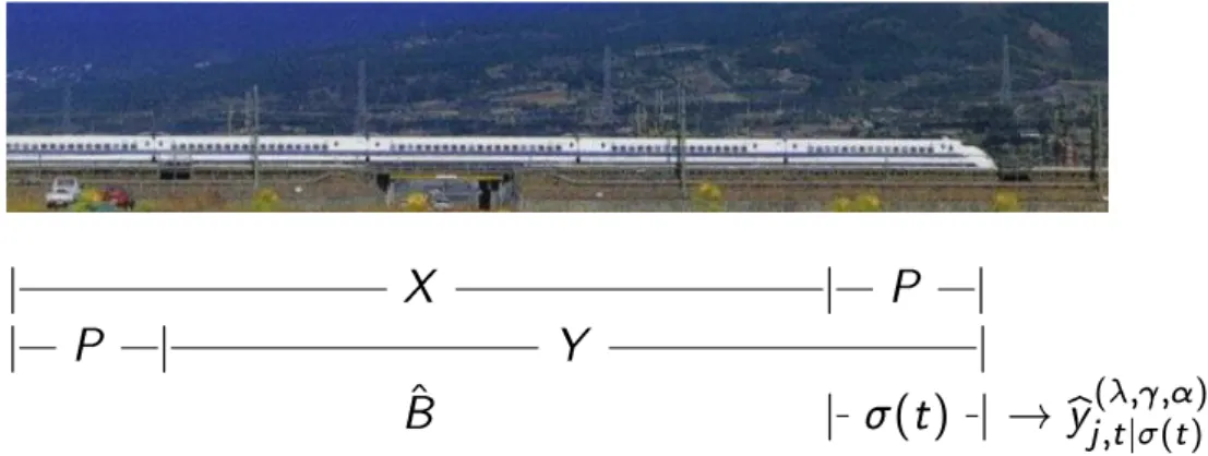
Figure 2: Illustration of the Rolling Scheme
evaluation sample respectively. The point estimate of thejth variable’s forecast is denoted by ybj,t(λ,γ,α|σ(t))
based on σ(t), the information up to time t. The point estimate of the one-step-ahead forecast is computed as in equation (5), and the h-step-ahead forecasts are computed in similar spirit. Out-of-sample forecast accuracy is measured in terms of mean squared forecast error (MSFE):
M SF Ej,h(λ,γ,α) = 1 T1−T0−h+ 1 T1−h X t=T0 (yb(j,tλ,γ,α+h|σ)(t)−yj,t+h|σ(t))2.
We report results for MSFE relative to the benchmark (random walk with drift) model’s (abbreviated asM SF Ej,h(0)), as also considered by Ba´nbura et al. (2010), i.e.
RM SF Ej,h(λ,γ,α)= M SF E
(λ,γ,α)
j,h M SF Ej,h(0) .
The parameters are estimated using the observations from the most recent 10 years (rolling scheme) as illustrated in Figure 2. The parameters are set to yield a desired fit for the variable(s) of inter-est from T0 to T1. In other words, to obtain the desired magnitude of fit, the search is performed over a grid of λ, γ and α to minimize PJ
j=1RM SF E
(λ,γ,α)
j,h (universal grouping); λj, γj and α to
minimize RM SF Ej,h(λ,γ,α) (no grouping); λi, γi, ηi and α to minimize P
j∈NiRM SF E
(λ,γ,η,α)
j,h
(segmen-tized grouping) respectively. Due to computational cost, we prefix α to be 1 or 2 first, and then do the search of λ’s and γ’s over loose grids. For the nice performing λ’s and γ’s, we search over denser grids around them afterwards. The parfor command in Matlab is used to facilitate parallel computations to fasten this process. Also, using the least angle regression package provided at www-stat.stanford.edu/∼tibs/glmnet-matlab, makes the computation time together with the parameter selection very moderate in our experience.
2.6
Algorithm
• P = diag[1α,2α, . . . , Pα]⊗IJ×J, where diag[1α,2α, . . . , Pα] is the diagonal matrix with diagonal
entries {1−α,2−α, . . . , P−α},⊗ is the Kronecker product andI
J×J is theJ×J identity matrix;
• W =IP×P ⊗diag[w1, w2, . . . , wJ];
• X˜>=X>W−1P−1 and ˜B =PWB
and note the fact that X>B in (2) is the same as X>W−1P−1PWB = ˜X>B˜, we have the following estimation procedure (the proof is very simple and hence is omitted):
(1) Generate ˜X> =X>W−1P−1;
(2) Corresponding to the three different estimates (4), (5) and (7), solve:
min ˜ B {J(T −P)}−1 T X t=P+1 kYt>−X˜t>B˜k2 2+λ P X p=1 J X j=1 kB˜pj−jk2+γ P X p=1 J X j=1 |B˜pjj|, (8) min ˜ B··j (T −P)−1 T X t=P+1 (Ytj −X˜t>B˜··j)2+λj P X p=1 X i6=j |B˜pij|+γj P X p=1 |B˜pjj|, (9) min B··Ni {Ni(T −P)}−1 T X t=P+1 kYt>Ni −Xt>B˜··Nik 2 2 +λNi P X p=1 X j /∈Ni kB˜pj·k2+γNi P X p=1 |B˜pjj| +ηNi P X p=1 X j∈Ni kB˜pj−jk2; ; (10)
(3) Output ˆB = W−1P−1Bˆ˜ with Bˆ˜ minimizing (8) (universal grouping), Bˆ˜ = (Bˆ˜
··1, . . . ,Bˆ˜··J),
ˆ ˜
B··j minimizing (9) (no grouping); Bˆ˜ = (Bˆ˜··N1, . . . ,
ˆ ˜ B··NI), ˆ ˜ B··Ni minimizing (10) (segmentized grouping).
At Step (2), motivated by Wang et al. (2007), as we have more than one penalty terms (mixed Lasso and group Lasso), we could iterate between penalties to solve it as the standard (group) Lasso problem.
For the “no grouping” estimate, by noting that γj = µjλj and γjPPp=1|B˜pjj| =λjPPp=1|µjB˜pjj|,
the estimation procedure above is equivalent to: (1) Generate ˜X> =X>W0−1P−1 with W0 = I
P×P ⊗diag[w1, w2, wj−1, ujwj, wj+1, . . . , wJ] for
esti-matingB··j,16j 6J; (2) Corresponding to (9), solve: min ˜ B··j (T −P)−1 T X t=P+1 (Ytj −X˜t>B˜··j)2+λj P X p=1 J X i=1 |B˜pij|; (11)
(3) Output ˆB =W0−1P−1B˜ˆ with Bˆ˜ = (Bˆ˜
··1, . . . ,Bˆ˜··J), Bˆ˜··j minimizing (9) (no grouping).
At Step (2), we could avoid iterating between multiple penalties and just solve it as the standard Lasso, e.g. by using the least angle regression package provided at www-stat.stanford.edu/∼ tibs/glmnet-matlab.
In “large J, small T” paradigms, to get parsimonious models, shrinkage with penalization in model selection can shrink insignificant regression coefficients towards zero exactly, but at the same time, significant coefficients are shrunk as well though they are retained in selected working models, Wainwright (2009) and Huang et al. (2008). To this end, we only use our method for the variable (and lag) selection, but not for estimation, Chernozhukov et al. (2011). Thus, we implement the ordinary least squares estimation for the selected variables (and lags) from (8), (9) and (10) w.r.t. three different estimates.
2.7
Comparison
Now it is a matter of what kind of regularization techniques among these three choices to use in practice. First, as already discussed in Remark 2.2.1 and 2.3.1, from the allowing individualized (for the variable of particular interest) weights between own lags and others’ lags and individualized forecasting performance optimization point of view, the “no grouping” approach is the best, the “universal grouping” one is the worst, and the “segmentized grouping” one is in between. Second, as in Remark 2.2.2 and 2.3.2, from whether all off-diagonal autocoefficients in one row are shrunk to zero point of view, the “no grouping” one is still favored. Third, as in subsection 2.5, the tuning parameters w.r.t. the universal grouping, no grouping or segmentized grouping estimates are selected to optimize the averaged forecasting performance for all variables, the specific variable’s forecasting performance or the averaged forecasting performance for the variables in the same segment respectively. When different variables’ time series have very distinct patterns, this individualized optimization is preferred.
Fourth, for the estimation of large coefficient matrices, due to the stronggroup-sparse assumption on the underlying structure as mentioned in subsection 2.2, the group lasso type estimator actually has a sharper theoretical risk bound, Huang and Zhang (2009) for more details. In particular, they show that group Lasso is more robust to noise due to the stability associated with group structure and thus requires a smaller sample size to satisfy the sparse eigenvalue condition required in modern sparsity analysis. And the universal grouping estimate is also more computationally efficient since the whole autocoefficient matrix is estimated at once. However, note that the statistical error is a combination of modeling error and estimation error. Even though the group Lasso type estimate might have smaller
estimation error, due to the strong assumption to the underlying structure, the overall risk might not be smaller, as we discussed in subsection 2.2. Moreover, the typical macroeconomic data has low frequency, i.e. monthly. Thus the computational cost is not a severe problem since we only need to update the model once per month at most. Due to all these, we suggest the no grouping estimate for practical implementation as a compromise between flexibility and realization of assumptions. For this reason and technical simplicities, we mainly study the theoretical properties of the no grouping estimate as defined in (6) afterwards.
3
Estimates’ Properties
In this section, we first show that, under the time series setup, if we just use the classic Lasso estimator, the risk bound will depend on the time dependence level as in Theorem 3.1. To circumvent this problem, through reweighting over time, our estimate in (6) can still produce an estimator, which is shown in Theorem 3.2 and 3.3, to be equivalent to an appropriate oracle. The techniques of the proofs are closely built upon those in Lounici et al. (2009), Bickel et al. (2009), Lounici (2008) and Wang et al. (2007).
3.1
Dependence Matters?
Now we will illustrate how the temporal dependence level affects the risk bounds of the Lasso type estimator. For technical simplicities, we consider the univariate AR(P) (or MA(P)) model with
P → ∞, i.e. J = 1 for equations (1) and (2):
et =xt1θ1+. . . , xtPθP +t=x>t θ+t, (12)
with the regressors (xt1, . . . , xtP) = xTt, the coefficients (θ1, . . . , θP) = θ> and the error term t. We
also define x as a T ×P matrix with the t, pth entry as xtp and e = (e1, . . . , eT)>. xtp = et−p (or t−p) corresponds to the AR(P) (or MA(P)) model. In this situation, since there are no “others lags”
(J = 1) and θ is a vector, the standard Lasso estimator ˆθ is defined through:
min θ (T −P) −1 T X t=P+1 (et−x>tθ)2+ 2λkθk1. (13)
We assume there is a true coefficient θ∗ for (12) and define M(θ∗) = Pp
p=11(θ
∗
p 6= 0) and M(ˆθ) = Pp
p=11(ˆθp 6= 0). Before moving on, we recall the fractional cover theory based definition first, which was introduced by Janson (2004) and can be viewed as a generalization of m-dependency. Given a setT and random variables Vt, t∈ T, we say:
• A subsetT0 ofT isindependentif the corresponding random variables{V
t}t∈T0 are independent.
• A family{Tj}j of subsets of T is a cover of T if S
jTj =T.
• A family{(Tj,wj)}j of pairs (Tj,wj), where Tj ⊆ T and wj ∈[0,1] is a fractional cover of T if P
jwj1Tj >1T, i.e. P
j:t∈Tjwj >1 for each t ∈ T.
• A (fractional) cover is proper if each set Tj in it is independent.
• X(T) is the size of the smallest proper cover of T, i.e. the smallest m such thatT is the union of m independent subsets.
• X∗(T) is the minimum of P
jwj over all proper fractional covers{(Tj,wj)}j.
Notice that, in spirit of these notations, X(T) and X∗(T) depend not only on T but also on the family {Vt}t∈T. Further note that X∗(T)> 1 (unlessT =∅) and that X∗(T) = 1 if and only if the
variables Vt, t ∈ T are independent, i.e. X∗(T) is a measure of the dependence structure of {Vt}t∈T. For example, if Vt only depends on Vt−1, . . . , Vt−k but is independent of all {Vs}s<t−k, we will have k+ 1 independent sets: T1 ={V1, V(k+1)+1, V2(k+1)+1, . . .}, T2 ={V2, V(k+1)+2, V2(k+1)+2, . . .}, . . . Tk+1 ={Vk+1, V(k+1)+(k+1), V2(k+1)+(k+1), . . .}, s.t. Sk+1 j=1Tj =T. So X∗(T) =k+ 1 (if k+ 1< T).
Before stating the first main result of this section, we make the following two assumptions.
ASSUMPTION 3.1 With a high probability q, ∀ p, the random variables xtp and t satisfy
|txtp|6bt and T−1 T X
t=1
b2t 6C0
for some constants bt, C0 >0, t= 1, . . . , T.
ASSUMPTION 3.2 There exists a positive number κ=κ(s) such that
minn |x >∆| 2 √ T|∆R|2 :|R|6s,∆∈RP\{0},k∆Rc k163k∆Rk1 o >κ,
where Rc denotes the complement of the set of indices R, ∆R denotes the vector formed by the
Assumption 3.2 is the restricted eigenvalue assumption from Bickel et al. (2009), which is essentially a restriction on the eigenvalues of the Gram matrix ΨT =x>x/T as a function of sparsitys. To see
this, recall the definitions of restricted eigenvalues and restricted correlations in Bickel et al. (2009):
ψmin(u) = min z∈RP:16M(z)6u z>ΨTz |z|2 2 , 16z6P, ψmax(u) = max z∈RP:16M(z)6u z>ΨTz |z|2 2 , 16z6P, ψm1,m2 = max nf> 1 x > I1xI2f2 T|f1|2|f2|2 :I1 \ I2 =∅,|Ii|6mi, fi ∈RIi\{0}, i= 1,2 o ,
where |Ii| denotes the cardinality of Ii and xIi is the T × |Ii| submatrix of x obtained by removing
from x the columns that do not correspond to the indices in Ii. Lemma 4.1 in Bickel et al. (2009)
shows that if the restricted eigenvalue of the Gram matrix ΨT satisfies ψmin(2s) > 3ψs,2s for some
integer 16s6P/2, Assumption 3.2 holds. We can now state our first main result.
THEOREM 3.1 Consider the model (12) forP >3, T >1 and random variablesVt=txtp, t∈ T.
Let the random variables xtp and t satisfy Assumption 3.1 for any p, all diagonal elements of the
matrix x>x/T euqal to 1, and M(θ∗)6 s. Furthermore, let κ be defined as in Assumption 3.2, and
φmax be the maximum eigenvalue of the matrix X>X/T. Let λ= p
X∗(T)(logP)1+δ0
C0/T , δ0 >0.
Then with probability at least q(1−P−δ0), for any solution θˆof (13), we have:
T−1kx(ˆθ−θ∗)k2 616sX∗(T)(logP)1+δ0C0/T κ2, (14) kθˆ−θ∗ k1 616616s p X∗(T)(logP)1+δ0 C0/T /κ2, (15) M(ˆθ)664φ2maxs/κ2. (16) Before explaining the results, we would like to discuss some related results first. Suppose x in (12) has full rank P and t is N(0, σ2). Consider the least squares estimate (P 6 T) ˆθOLS = (xx>)−1xe.
Then from standard least squares theory, we know that the prediction error kxT(ˆθOLS −θ∗)k22/σ2 is
χ2 p-distributed, i.e. E kx T(ˆθ OLS −θ∗)k22 T = σ2 T P. (17)
In the sparse situation iftis N(0, σ2) (different from our case), Corollary 6.2 of B¨uhlmann and van de
Geer (2011) shows that the Lasso estimate obeys the following oracle inequality:
kxT(ˆθLasso−θ∗)k22 T 6C0 σ2logP T M(θ ∗ ) (18)
with a large probability and some constantC0. The additional logP factor here could be seen as the price to pay for not knowing the set{θp∗, θp∗ 6= 0}, Donoho and Johnstone (1994).
Similar to the i.i.d. Gaussian situation discussed above, the term s(logP)1+δ0 in (20) could be interpreted as the price to pay for not knowing the set {θ∗p, θ∗p = 06 }. Here we have (logP)1+δ0 instead
of logP because we deviate from the typical i.i.d. Gaussian situation and establish the result under the more general Assumption 3.1, which could be thought as the “finite second moment” condition. And the δ0 term is the price to pay for this deviation.
For the case ofxtp =t−p(MA(P) model), by the definition ofX∗(T) andVt, ifk∗ = max{p,s.t.θ∗p 6=
0, θ∗p+1 =θp∗+2 =. . .=θP∗ = 0}), we have X∗(T) =k∗+ 1 (if k∗+ 1 < T). The RHS of (14) becomes 16s(k∗+ 1)(logP)1+δ0/T κ2. For the case ofx
tp =et−p (AR(P) model), which is equivalent to MA(∞)
and X∗(T)
6T, the RHS of (14) becomes 16s(logP)1+δ0/κ2. Thus X∗(T) could be interpreted as a measure on how many past lagsVtdepends on. Additionally, when the time dependence level increases,
by the definition of the Gram matrix, κ will decrease since it characterizes how strong xt1, . . . , xtP
depend on each other. Still using the MA(k∗) example considered above, κ could be thought as a measure on how strongetdepends on et−1, . . . , et−k∗, which is a complement of the measure ofX∗(T)
on the time dependence level. In both cases (MA(P) or AR(P)), Theorem 3.1 states that if we use the standard Lasso estimate directly for the time series, the bounds get larger when the dependence level (X∗(T)) increases and κ decreases. In other words, the bound is minimized when X∗(T) = 1, which corresponds to the independent situation in the literature. When X∗(T) reaches T, it will be offset by the T in the denominator. Thus the risk bound does not decrease when T increases. The intuition behind is clear: if the dependence level is strong, then the additional information brought by a “new” observation will be effectively less, i.e. the overall information from {Vt}Tt=1 will be less correspondingly, which will result in increasing estimates’ risk bounds. Consequently, we expect the selection not to be stable and to be very sensitive to minor perturbation of the data. In this sense, we do not expect variable selection to provide results that lead to clearer economic interpretation than principal components or Ridge regression.
3.2
Consistency of Selection
To study the oracle properties of the estimator in (6), we assume that there is a correct model with the regression and autoregression coefficients β∗ = (c∗>, d∗>)> = (c∗1, . . . , c∗P(J−1), d∗1, . . . , d∗P)0. Furthermore, we assume that there are a total of p0 6 P(J −1) non-zero other-lag coefficients and
q0 6 P non-zero own-lag coefficients. For convenience, we define S1 = {1 6 i 6 P(J −1), c∗i 6= 0},
ˆ
S1 ={16i6P(J−1),ˆci 6= 0}, S2 ={16p6P, d∗p 6= 0} and ˆS2 ={16p6P,dˆp 6= 0}. Then, the
sets S1 and S2 contain the indices of the significant others-lag and own-lag coefficients respectively, and their complements S1c and S2c contain the indices of the insignificant coefficients. Next, let
c∗S1 denote the p0 ×1 significant other-lag coefficient vector with ˆcS1 being its associated estimator.
Moreover, other related parameters and their corresponding estimators are analogously defined (e.g.
c∗Sc 1,cˆS c 1, d ∗ S2, ˆ dS2, d ∗ Sc 2, ˆ dSc2). Finally, letβ ∗ 1 = (c∗ 0 S1, d ∗0 S2) 0andβ∗ 2 = (c∗ 0 Sc 1, d ∗0 Sc 2)
0with corresponding estimates ˆ
β1,βˆ2. To facilitate the study, we also introduce the notations
aT def = max(λi, γp, i∈S1, p∈S2), bT def = min(λi, γp, i∈S1c, p∈S c 2),
where λi and γp are functions of T. To investigate the theoretical properties of ˆβ, we introduce the
following conditions:
A1 The sequence {Xt} is independent of εt (εt
def = Utj);
A2 All roots of polynomial 1−PP
p=1d
∗
pzp are outside the unit circle;
A3 εt has finite fourth-order moment, i.e. E(ε4t)<∞;
A4 ∀j, Ytj (as components of the covariateXt) is strictly stationary and ergodic with finte
second-order moment (i.e. EkYtjk2 <∞).
The technical conditions above are typically used to assure the √T-consistency and asymptotic nor-mality of the unpenalized least squares estimator.
We also rewrite equation (6) as min β QT(β) = minβ T X t=P+1 (yt−Xt>β) 2+T P(J−1) X i=1 λi|ci|+T P X p=1 γp|dp| (19)
by multiplying 2(T −P) and writing T −P as T without confusion. Define PT
t=P+1(yt−X
>
t β)2 as
LT(β),xTt = (Xj,t, X2j,t, . . . , XJ j,t), the own lags corresponding to the coefficientsc, andzt> =Xt>\x>t ,
others’ lags corresponding to the coefficients d respectively. Then Xt>β=x>t c+zt>d. We first investigate the consistency of the estimator of (6).
LEMMA 3.1 Assume that aT = O(1) as T → ∞. Then, under conditions (A1-A4), ∃ a local
minimizer βb of (6) s.t.
kβb−β∗k=Op(T−1/2+aT).
The proof is given in the appendix. Lemma 3.1 implies that, if the tuning parameters associated with the significant regressors converge to 0 at a speed faster than T−1/2, then there is a local minimizer of (6), which is √T-consistent. Next, we show that, if the tuning parameters associated with the insignificant regressors shrink to 0 slower thanT−1/2, then their coefficients can be estimated exactly as 0 with probability tending to 1.
THEOREM 3.2 (Consistency of Selection) Assume thatbT √
T → ∞andkβb−β∗k=O(T−1/2),
then
P(βb2 = 0)→1.
Theorem 3.2 shows that our method can produce a sparse solution for insignificant coefficients con-sistently. Furthermore, this theorem, together with Lemma 3.1, indicates that the √T-consistent estimator must satisfy P(βb2 = 0)→1 when the tuning parameters fulfill the appropriate conditions. Finally, we obtain the asymptotic distribution of this estimator.
THEOREM 3.3 Assume that aT √
T → 0 and bT √
T → ∞. Then, under conditions (A1-A4), the “nonzero” components βb1 of the local minimizer βbin Lemma 3.1 satisfies
(βb1 −β1∗)
√
T →d N(0,Σ−10 ),
P( ˆS1 =S1)→1, P( ˆS2 =S2)→1,
where Σ0 is the submatrix of Σ corresponding to β1∗, Σ = diag(B, C), B =E(xtx>t ) and C=E(ztzt>).
Theorem 3.3 implies that, if the tuning parameters satisfy the conditionsaT √
T →0 andbT √
T → ∞, then, asymptotically, the resulting estimator can be as efficient as the oracle estimator. And our method can produce a sparse solution for significant coefficients consistently.
Since consistency of selection is established here, if we use the ordinary least squares estimation for the selected variables, we can avoid the log term on (18) and (14).
4
Application
We use the dataset of Stock and Watson (2005a) for illustration. This dataset contains 131 monthly macro indicators covering a broad range of categories including income, industrial production, ca-pacity, employment and unemployment, consumer prices, producer prices, wages, housing starts, inventories and orders, stock prices, interest rates for different maturities, exchange rates, money aggregates and so on. The time span is from January 1959 to December 2003. We apply logarithms to most of the series except those already expressed in rates. The variables of special interest include a measure of real economic activity, a measure of prices and a monetary policy instrument. As in Christiano et al. (1999), we use employment as an indicator of real economic activity measured by the number of employees on non-farm payrolls (EMPL). The level of prices is measured by the consumer price index (CPI) and the monetary policy instrument is the Federal Funds Rate (FFR). All 131
P = 1 P = 4 P = 7 P = 13 P = 25 BVAR EMPL 0.3333 0.3336 0.3338 0.3341 0.3335 0.46 h= 1 CPI 0.3623 0.3618 0.3613 0.3621 0.3623 0.50 FFR 0.4279 0.4281 0.4281 0.4284 0.4287 0.75 EMPL 0.5191 0.5188 0.5192 0.5191 0.5189 0.38 h= 3 CPI 0.4990 0.4992 0.4986 0.4995 0.4996 0.40 FFR 0.4615 0.4614 0.4619 0.4617 0.4628 0.94 EMPL 0.4730 0.4730 0.4735 0.4729 0.4736 0.50 h= 6 CPI 0.4880 0.4874 0.4884 0.4885 0.4891 0.40 FFR 0.5237 0.5242 0.5243 0.5243 0.5250 1.29 EMPL 0.4997 0.4991 0.4992 0.4997 0.5002 0.78 h= 12 CPI 0.4689 0.4687 0.4689 0.4694 0.4686 0.44 FFR 0.4201 0.4199 0.4201 0.4200 0.4216 1.93
Table 1: RMSFE w.r.t. different choices of h and P.
variables’ lags are used as regressors. As discussed earlier, because of the stationary requirement of our method, the series are transformed to obtain stationarity so that many of the series are (2nd order) differences of the raw data series (or logarithm of the raw series).
We evaluate the forecast performance over the period from T0 = January 70 to T1 = December 03 and for forecast horizons up to one year (h = 1,3,6,12). The order of the VAR is set to be
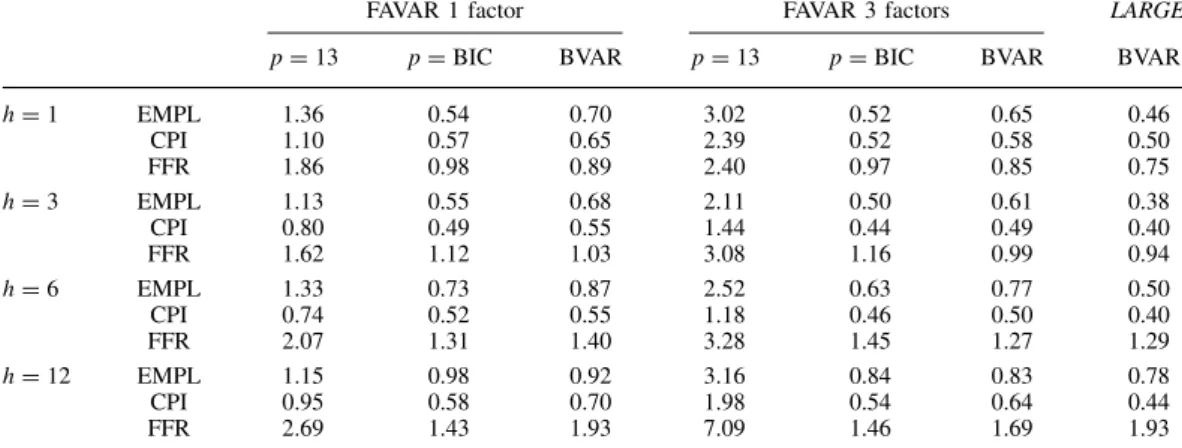
P = 1,4,7,13,25. The resulting performance is summarized in Table 1 with comparisions to the ones of Ba´nbura et al. (2010) listed under the “BVAR” column. As we can see, unlike the information criteria based on lag selection techniques, the RMSFE is very robust to the initial choice ofP, which primarily benefits from the “re-weighting over lags” technique (p−α) we used before. For this specific data set, P = 1 seems enough. But in general, since we never know the true value of lags, we can include a large enough P at the beginning to allow flexibility without worrying about over fitting. Moreover, for the one-step-ahead forecast, our method outperforms for EMPL, CPI and FFR, while when h > 3, it outperforms mainly for EMPL and FFR, especially for the latter one. This results from the fact that different time series might have quite different behaviors, so if we just have the “universal” penalty parameter for all of them as in Ba´nbura et al. (2010), the corresponding forecasting performance might not be optimized. For reference purpose, we also provide the factor-augmented vector autoregressive results of Bernanke et al. (2005) in Figure 3.
LARGE BAYESIAN VARS 81
Table III. FAVAR, relative MSFE, 1971 –2003
FAVAR 1 factor FAVAR 3 factors LARGE pD13 pDBIC BVAR pD13 pDBIC BVAR BVAR
hD1 EMPL 1.36 0.54 0.70 3.02 0.52 0.65 0.46 CPI 1.10 0.57 0.65 2.39 0.52 0.58 0.50 FFR 1.86 0.98 0.89 2.40 0.97 0.85 0.75 hD3 EMPL 1.13 0.55 0.68 2.11 0.50 0.61 0.38 CPI 0.80 0.49 0.55 1.44 0.44 0.49 0.40 FFR 1.62 1.12 1.03 3.08 1.16 0.99 0.94 hD6 EMPL 1.33 0.73 0.87 2.52 0.63 0.77 0.50 CPI 0.74 0.52 0.55 1.18 0.46 0.50 0.40 FFR 2.07 1.31 1.40 3.28 1.45 1.27 1.29 hD12 EMPL 1.15 0.98 0.92 3.16 0.84 0.83 0.78 CPI 0.95 0.58 0.70 1.98 0.54 0.64 0.44 FFR 2.69 1.43 1.93 7.09 1.46 1.69 1.93
Notes: The table reports MSFE for the FAVAR model relative to that from the benchmark model (random walk with drift) for employment (EMPL), CPI and federal funds rate (FFR) for different forecast horizonsh. FAVAR includes 1 or 3 factors and the three variables of interest. The system is estimated by OLS with number of lags fixed to 13 or chosen by the BIC and by applying Bayesian shrinkage. For comparison the results from large Bayesian VAR are also provided.
Let us rewrite the VAR of equation (1) in its error correction form:
Yt DcInA1. . .ApYt1CB1Yt1C. . .CBp1YtpC1Cut 8 A VAR in first differences implies the restrictionInA1. . .ApD0. We follow Doan
et al. (1984) and set a prior that shrinksDInA1. . .Apto zero. This can be understood as ‘inexact differencing’ and in the literature it is usually implemented by adding the following dummy observations (cf. Section 2):
YdDdiagυ11, . . . , υnn/ XdD11ðpdiagυ11, . . . , υnn/ 0nð1 9
The hyperparameter controls for the degree of shrinkage: as goes to zero we approach the case of exact differences and, as goes to 1, we approach the case of no shrinkage. The parameteri aims at capturing the average level of variableyit. Although the parameters should in principle be set using only prior knowledge, we follow common practice5and set the parameter
equal to the sample average ofyit. Our approach is to set a loose prior with D10. The overall shrinkageis again selected so as to match the fit of the small specification estimated by OLS.
Table IV reports results from the forecast evaluation of the specification with the sum of coefficient prior. They show that, qualitatively, results do not change for the smaller models, but improve significantly for the MEDIUM and LARGE specifications. In particular, the poor results for the federal funds rate discussed in Table I are now improved. Both theMEDIUM and
LARGE models outperform the random walk forecasts at all the horizons considered. Overall, the sum of coefficient prior improves forecast accuracy, confirming the findings of Robertson and Tallman (1999).
5See, for example, Sims and Zha (1998).
Copyright2009 John Wiley & Sons, Ltd. J. Appl. Econ.25: 71– 92 (2010) DOI: 10.1002/jae
Figure 3: Results of Bernanke et al. (2005) and Ba´nbura et al. (2010)
5
Concluding Remarks and Discussions
To summarize, in this article, we first show that under the time series setup, if we still use the classic Lasso type estimator, the risk bound will increase when the time dependence level increases, however, our method could still achieve the consistency of variable selection under such scenario; second, our method is able to do variable selection and lag selection simultaneously, and is rather robust to the initial choice of lags; third, we allow individualized weights between own and others’ lags. All these have been confirmed by the real forecasting performance in the previous section and come at a low computational cost.
Some issues we do not explore here include nonstationarity, rank test, cointegration and causal test. For a typical macroeconomic data set, the nonstationarity comes from seasonality, business cycle and economic developments. In spirit of Song et al. (2010), this motivates us to add a nonstationary component UΓ to equation (2) as below
Yt =ZtΓ +XtB+Ut,
where Zt = (Z1(t), . . . , ZR(t))> contains R basis functions of time consisting of Fourier series with
different frequencies and segment by segment ortho-normal polynomials with corresponding R×J
coefficient matrix Γ, andXt, B are the same as in equation (1). Studying this extended model deserves
further investigation and will be presented in a separate paper. If we want to consider the rank test, cointegration and causal test, what we need for this high dimensional time series is not the ones in the univariate case, but the high dimensionalsimultaneous tests, which might be much more difficult.
Heteroscedasticity with Cross-section Correlations.
We consider Cov(Ut) = Σ with nonzero off-diagonal entries in Σ. Assume that we have a
consis-tent estimate ˆΣ for Σ (which is another challenging task since Σ is a J ×J matrix) with Cholesky decomposition ˆΣ = C>C, where C is an upper triangular matrix with inverse D (which is also an
upper triangular matrix). Without loss of generality, assume all diagonal entries of ˆΣ, C and D are equal to 1. Transform the original Xt by D to generate ˜Xt ( ˜Xt = XtD) s.t. Cov(UtD) =I. Under
this situation, we are no longer selecting the original variables, but linear transformations of them. Thus we must show that this does not affect the inference. We have
˜ β1x˜t1+ ˜β2x˜t2+. . .+ ˜βJx˜tJ = ˜β1xt1+ ˜β2(d12xt1+xt2) +. . .+ ˜βJ( J−1 X j=1 djJxtj +xtJ) =( ˜β1+ J X j=2 ˜ βjd1j)xt1+ ( ˜β2+ J X j=3 ˜ βjd2j)xt2+. . .+ ˜βJxtJ.
If the off-diagonal entries ofD,{dij}i<j, are much smaller than the diagonal entries 1, it is likely that
the selected nonzero sets of ˜β’s (or ˜c,d˜) are the same as the selected nonzero sets ˆS1 and ˆS2 of β’s, which have been shown to be the same as the oracle ones, Theorem 3.2 and 3.3. By the definition of D, this means that the off-diagonal entries of C,Σ and Σ should also be much smaller than theirˆ diagonal entries 1, e.g. the cross-section correlations must be weak enough, which aligns with the case for dynamic factor models, Forni et al. (2000).
Acknowledgement The main results of this paper were first presented at the annual Winter Meeting of the Econometric Society, Denver, Jan, 2011. We are grateful for seminar participants’ many interesting comments on several versions of the paper. In particular, I would like to thank Prof Peter Bickel for sponsoring my stay at the University of California, Berkeley. This work is also partially supported by Deutsche Forschungsgemeinschaft via SFB 649 “ ¨Okonomisches Risiko”, Humboldt-Universit¨at zu Berlin from May, 2011 to Oct, 2011, which is greatly acknowledged. We would also like to thank Prof Marta Ba´nbura, Prof Domenico Giannone and Prof Lucrezia Reichlin for sharing the codes of BVAR.
6
Appendix
Proof of Theorem 3.1The proof of this theorem is based on the ones of Lemma 3.1 and Theorem 3.1 in Lounici et al. (2009) up to a modification of the bound on P(Ac) with random event A = n
max16p6PPTt=1εtXtp 6λT o
The intermediate results in the proof of Theorem 3.1 in Lounici et al. (2009) show that T−1kX(Bb−B∗)k 2 616sλ2/κ2, (20) kBb−B∗ k616616sλ/κ2, (21) M(Bb)664φ2maxs/κ2. (22) We have: P(Ac) = P max 16p6P T X t=1 εtXtp> λT 6PP T X t=1 εtXtp > λT def = PP T X t=1 Vt> λT .
Then, by the (extended) Mcdiarmid inequality, see Theorem 2.1 of Janson (2004), with random vectors{Vt}Tt=1, we have P(Ac)6P P XT t=1 Vt> λT 6P exp − λ 2T X∗(T)P tb2t/T 6P−δ0 with λ =pX∗(T)(logP)1+δ0
C0/T , δ0 > 0, which, together with (20), (21) and (22), leads to (14),
(15) and (16).
Proof of Lemma 3.1 The proofs are closely built upon those of Wang et al. (2007). Let δ = (u>, v>)>, u = (u1, . . . , uP(J−1))>, v = (v1, . . . , vP)>, αT = T−1/2 +an and {β∗+αTδ : kδk 6 e} be
the ball around β∗. Then, for kδk=e, we have
DT(δ) =QT(β∗+αTδ)−QT(β∗) =LT(β∗+αTδ)−LT(β∗) +T X i∈S1 λi(|c∗i +αTui| − kc∗ik) +T X j∈S2 γj(|d∗j +αTvj| − kd∗jk) =LT(β∗+αTδ)−LT(β∗)−T αT X i∈S1 λi|ui| −T αT X j∈S2 γj|vj| =LT(β∗+αTδ)−LT(β∗)−T α2Tp0e−T α2Tq0e =LT(β∗+αTδ)−LT(β∗)−T α2T(p0+q0)e. (23) Furthermore, LT(β∗+αTδ)−LT(β∗) = X t {ut−aTz>t v−aTu>xt}2− X t u2t = a2T X t {(zt>v)2 +u>xtx>t u} (24) −2aT X t utzt>v (25) +2a2T X t zt>vu>xt. (26)
By employing the martingale central limit theorem and the ergodic theorem, we can show that (24) =T a2
T{δ
>Σδ+
Op(1)}, (25) =δ>Op(T a2T) and (26) =T a2TOp(1) =Op(T a2T). Because (24) dominates the terms (25), (26) andT α2T(p0+q0)ein equation (23), for any given >0, there is a large constant
e such that
P[ inf
kδk=eQT(β
∗
+αTδ)> QT(β∗)]>1−.
This implies that, with probability at least 1−, there is a local minimizer in the ball {β∗ +αTδ : kδk 6 e}, Bickel et al. (1998) and Fan and Li (2001). Consequently, there is a local minimizer of
QT(β) such that kβˆ−β∗k=Op(αT). This completes the proof.
Proof of Theorem 3.2 The proof is essentially the same as those of Theorem 2 of Zou (2006) and Wang et al. (2007). For i ∈ S1c, assume that there is a local minimizer ˆβ with ˆci 6= 0. By the KKT
optimality condition, we have
0 = ∂LT( ˆβ) ci +T λisgn(ˆci) = ∂LT(β ∗) ci +TΣi( ˆβ−β∗){1 +Op(1)}+T λisgn(ˆci), (27)
where Σi denotes the ith row of Σ and i∈S1c. By employing the central limit theorem, the first term in equation (27) is of order Op(T1/2). Furthermore, the condition in Theorem 3.2 implies that its
second term is also of orderOp(T1/2). Both are dominated by T λi since bT √
T → ∞. Therefore, the sign of equation (27) is dominated by the sign of ˆci. Thus (27) can not be equal to 0. Consequently,
we must have ˆci = 0 in probability. Analogously, we can show that P( ˆdSc
2 = 0)→1. This completes
the proof.
Proof of Theorem 3.3Applying Lemma 3.1 and Theorem 3.2, we have P(βb2 = 0)→1. Hence, the
minimizer of QT(β) is the same as that of QT(β1) with probability tending to 1. This implies that the estimator ˆβ1 satisfies the equation
∂QT(β1) β1 β1= ˆβ1 = 0. (28) According to Lemma 3.1, ˆβ1 is √
T-consistent. Thus, the Taylor series expansion of equation (28) yields 0 = √1 T ∂LT( ˆβ1) β1 +g( ˆβ1) √ T = √1 T ∂LT(β1∗) β1 +g(β1∗)√T + Σ0 √ T( ˆβ1−β1∗) +Op(1),
where g is the first-order derivative of the penalty function
X i∈S1 λi|ci|+ X j∈S2 γj|dj|,
and g( ˆβ1) =g(β1∗) when T is sufficiently large. Furthermore, it can be easily shown that g(β1∗)
√
T = Op(1), which implies that
( ˆβ1−β1∗) √ T = Σ −1 0 √ T ∂LT(β1∗) ∂β1 +Op(1) d → N(0,Σ−10 ).
The next step is to show P( ˆS1 =S1)→ 1 and P( ˆS2 = S2) →1. ∀i∈S1 and p∈ S2, the asymptotic normality result indicates that ˆci
p
→c∗i and ˆdp p
→d∗p, where →p stands for convergence in probability. Thus P(i∈Sˆ1)→1 and P(p∈Sˆ2)→1. It suffices to show that∀i0 ∈/S1 and p0 ∈/ S2, P(i0 ∈Sˆ1)→0 and P(p0 ∈Sˆ2)→0, which have been shown by Theorem 3.2. This completes the proof.
References
Ba´nbura, M., Giannone, D., and Reichlin, L. (2010). Large bayesian vector auto regressions. Journal of Applied Econometrics, 25(1):71–92.
Bernanke, B., Boivin, J., and Eliasz, P. S. (2005). Measuring the effects of monetary policy: A factor-augmented vector autoregressive (favar) approach. The Quarterly Journal of Economics, 120(1):387–422.
Bickel, P. J., Klaassen, C. A. J., Ritov, Y., and Wellner, J. (1998). Efficient and adaptive estimation for semiparametric models, 2nd edition. Springer Verlag.
Bickel, P. J., Ritov, Y., and Tsybakov, A. B. (2009). Simultaneous analysis of Lasso and Dantzig selector. Annals of Statists, 37(4):1705–1732.
B¨uhlmann, P. and van de Geer, S. (2011). Statistics for High-Dimensional Data: Methods, Theory and Applications. Heidelberg: Springer Verlag.
Chernozhukov, V., Belloni, A., and Hasen, C. (2011). Estimation and inference methods for high-dimensional sparse econometric models. Submitted.
Christiano, L., Eichenbaum, M., and Evans, C. (1999). Monetary policy shocks: What have we learned and to what end? Handbook of Macroeconomics, 1(1):65–148.
Chudik, A. and Pesaran, M. (2007). Infinite dimensional vars and factor models. Cambridge Working Papers in Economics 0757, Faculty of Economics, University of Cambridge.
Diebold, F. X. and Li, C. (2006). Forecasting the term structure of government bond yields. Journal of Econometrics, 130:337–364.
Doan, T., Litterman, R., and Sims, C. (1984). Forecasting and conditional projection using realistic prior distributions. Econometric Reviews, 3(1):1–100.
Donoho, D. L. and Johnstone, I. M. (1994). Ideal spatial adaptation by wavelet shrinkage. Biometrika, 81(3):pp. 425–455.
Efron, B., Hastie, T., Johnstone, L., and Tibshirani, R. (2004). Least angle regression. Annals of Statistics, 32:407–499.
Fan, J. and Li, R. (2001). Variable selection via nonconcave penalized likelihood and its oracle properties. Journal of the American Statistical Association, 96(456):1348–1360.
Fengler, M. R., H¨ardle, W., and Mammen, E. (2007). A semiparametric factor model for implied volatility surface dynamics. Journal of Financial Econometrics, 5(2):189–218.
Figlewski, S., Frydman, H., and Liang, W. (2006). Modeling the effect of macroeconomic factors on corporate default and credit rating transitions. NYU Stern Finance Working Paper No. FIN-06-007. Available at SSRN: http://ssrn.com/abstract=934438.
Forni, M., Hallin, M., Lippi, M., and Reichlin, L. (2000). The generalized dynamic-factor model: Identification and estimation. The Review of Economics and Statistics, 82(4):540–554.
Forni, M., Hallin, M., Lippi, M., and Reichlin, L. (2005). The generalized dynamic factor model: One-sided estimation and forecasting. Journal of the American Statistical Association, 100:830– 840.
Geweke, J. (1977). The dynamic factor analysis of economic time series. Latent Variables in Socio-Economic Models, eds. D. J. Aigner and A. S. Goldberg, Amsterdam: North-Holland, pages 365–383.
Giannone, D., Reichlin, L., and Sala, L. (2005). Monetary policy in real time. In NBER Macroeconomics Annual 2004, Volume 19, NBER Chapters, pages 161–224. National Bureau of Economic Research, Inc.
Huang, J., Ma, S., and Zhang, C. (2008). Adaptive lasso for sparse highdimensional regression. Statistica Sinica, 18:1603–1618.
Huang, J. and Zhang, T. (2009). The Benefit of Group Sparsity. ArXiv e-prints.
Janson, S. (2004). Large deviations for sums of partly dependent random variables. Random Structures Algorithms, 24(3):234–248.
Lee, R. D. and Carter, L. (1992). Modeling and forecasting the time series of u.s. mortality. Journal of the American Statistical Association, 87(419):659–671.
Lounici, K. (2008). Sup-norm convergence rate and sign concentration property of lasso and dantzig estimators. Electronic Journal of Statistics, 2:90–102.
Lounici, K., Pontil, M., Tsybakov, A. B., and van de Geer, S. (2009). Taking advantage of sparsity in multi-task learning. Proceedings of Conference on Learning Theory (COLT) 2009.
Mol, C. D., Giannone, D., and Reichlin, L. (2008). Forecasting using a large number of predictors: Is bayesian shrinkage a valid alternative to principal components? Journal of Econometrics, 146(2):318 – 328.
Myˇsiˇckov´a, A., Song, S., Mohr, P. N., Heekeren, H. R., and H¨ardle, W. K. (2011). Risk patterns and correlated brain activities. Working paper.
Nelson, C. R. and Siegel, A. F. (1987). Parsimonious modeling of yield curves. Journal of Business, 60:473–489.
Park, B. U., Mammen, E., H¨ardle, W., and Borak, S. (2009). Time series modelling with semipara-metric factor dynamics. Journal of the American Statistical Association, 104(485):284–298.
Sargent, T. J. and Sims, C. A. (1977). Business cycle modeling without pretending to have too much a priori economic theory. Working Papers 55, Federal Reserve Bank of Minneapolis.
Song, S., H¨ardle, W., and Ritov, Y. (2010). Dynamic factor models for high dimensional nonstationary time series. Under revision.
Stock, J. H. and Watson, M. W. (2002a). Forecasting using principal components from a large number of predictors. Journal of the American Statistical Association, 97:1167–1179.
Stock, J. H. and Watson, M. W. (2002b). Macroeconomic forecasting using diffusion indexes. Journal of Business & Economic Statistics, 20(2):147–62.
Stock, J. H. and Watson, M. W. (2005a). An empirical comparison of methods for forecasting using many predictors. Manuscript, Princeton University.
Stock, J. H. and Watson, M. W. (2005b). Implications of dynamic factor models for VAR anal-ysis. NBER Working Papers 11467, National Bureau of Economic Research, Inc. available at http://ideas.repec.org/p/nbr/nberwo/11467.html.
Tibshirani, R. (1996). Regression shrinkage and selection via the Lasso. Journal of the Royal Statistical Society, Series B, 58(1):267–288.
Wainwright, M. J. (2009). Sharp thresholds for high-dimensional and noisy sparsity recovery using l1-constrained quadratic programming (lasso). IEEE Trans. Inf. Theor., 55:2183–2202.
Wang, H., Li, G., and Tsai, C.-L. (2007). Regression coefficient and autoregressive order shrinkage and selection via the lasso. Journal Of The Royal Statistical Society Series B, 69(1):63–78.
Worsley, K., Liao, C., Aston, J., Petre, V., Duncan, G., Morales, F., and Evans, A. (2002). A general statistical analysis for fmri data. NeuroImange, 15:1–15.
Yuan, M. and Lin, Y. (2006). Model selection and estimation in regression with grouped variables. Journal of the Royal Statistical Society, Series B, 68(1):49–67.
Zou, H. (2006). The adaptive lasso and its oracle properties. Journal of the American Statistical Association, 101:1418–1429.