Rules of the Road: Predicting Driving Behavior With a Convolutional Model of Semantic Interactions

Rules of the Road:

Predicting Driving Behavior with a Convolutional Model of Semantic

Interactions

Joey Hong

∗

Caltech

[email protected]

Benjamin Sapp

∗ [email protected]

James Philbin

Zoox

[email protected]

Abstract

We focus on the problem of predicting future states of entities in complex, real-world driving scenarios. Previous research has used low-level signals to predict short time horizons, and has not addressed how to leverage key as-sets relied upon heavily by industry self-driving systems: (1) large 3D perception efforts which provide highly accu-rate 3D states of agents with rich attributes, and (2) detailed and accurate semantic maps of the environment (lanes, traf-fic lights, crosswalks, etc). We present a unified representa-tion which encodes such high-level semantic informarepresenta-tion in a spatial grid, allowing the use of deep convolutional mod-els to fuse complex scene context. This enables learning entity-entity and entity-environment interactions with sim-ple, feed-forward computations in each timestep within an overall temporal model of an agent’s behavior. We propose different ways of modelling the future as adistributionover future states using standard supervised learning. We intro-duce a novel dataset providing industry-grade rich percep-tion and semantic inputs, and empirically show we can ef-fectively learn fundamentals of driving behavior.

1. Introduction

A crucial component of real-world robotic systems is predicting future states of other actors in the environment. In the general setting, other actors’ intents are unobserved, thus the challenge is to produce a likely distribution over possible futures, given current and past observations. A motivating application for this work is a self-driving robot operating in an unconstrained urban environment; one of the most impactful yet challenging real-world robotics ap-plications today. It requires a deep understanding of the

∗_{Work done while at Zoox. The authors would also like to thank and} acknowledge Kai Wang ([email protected]) for his work on this project. Kai has been instrumental in coordinating the final version of the paper and preparing the dataset for release.

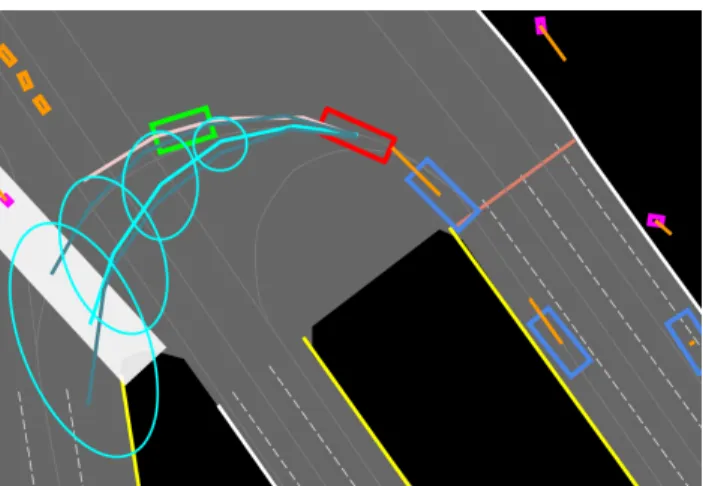
Figure 1: Entity future state prediction task on a top-down scene: A target entity of interest is shown in red, with a real future trajectory shown in pink. The most likely pre-dicted trajectory is shown in cyan, with alternate trajectories shown in green. Uncertainty ellipses showing 1 standard de-viation of uncertainty are displayed for the most likely tra-jectory only. Other entities are rendered in magenta (pedes-trians), blue (vehicles) and orange (bicycles). The ego vehi-cle which captured the scene is shown in green. Velocities are shown as orange lines scaled proportional to1m/s. Ex-amples of underlying semantic map information shown are lane lines, crosswalks and stop lines.

semantics of the static and dynamic environment, including understanding traffic laws, unspecified driving conventions, and interactions between human and robot actors.

While there is a large amount of research dedicated to real-world perception in this domain [15,25, 26,12, 35,

29,13,9], there is a surprising lack of work on entity state prediction in the same domain (see Section2), which we attribute to two main causes:

One, most previous research [25,22] takes as input only raw sensor information (a combination of camera, lidar or

1

radar). Thus the research effort by necessity requires a heavy emphasis on extracting high-level representations of entities. In contrast, in real-world systems in industry, low-level perception systems provide entity states and attributes from sensor data via detection and tracking in 2d and 3d. These systems are have matured over the past few years and have high fidelity output in the common case.

Two, publicly available datasets for learning and evalu-ating state prediction models are inadequately small and/or unrealistic. A good prediction dataset should include a diverse set of real-world locations and a large number of unique agent 3d tracks over meaningful time intervals. These criteria are necessary to develop models which can generalize to new scenarios and leverage past behavior to make meaningful future predictions out to 5 seconds or more. A final omission in previous prediction research is a key asset relied upon heavily by industry self-driving robots: semantic maps of the driving environment, as shown in Fig.1.

In this paper, we introduce a vehicle prediction dataset which is significantly richer and larger than existing datasets—9,659 unique vehicles in 83,880 prediction sce-narios (173 hours), in 88 physically-distinct locations—and includes semantic map information (see Figure1).

We propose a model which encodes a history of world state (both static and dynamic) and semantic map informa-tion in a unified, top-down spatial grid. This allows us to use a deep convolutional architecture to model entity dynamics, entity interactions, and scene context jointly.

An additional important contribution of this work is di-rectly predictingdistributionsof future states, rather than a single point estimate at each future timestep. Representing multimodal uncertainty is crucial in real-world planning for driving, which must consider vehicles taking different pos-sible trajectories, or assessing the expected risk of collision within some spatial extent.

We explore a variety of parametric and non-parametric output distribution representations, and show strong perfor-mance on predicting vehicle behavior up to 5 seconds in the future. We demonstrate that our model leverages road information and other agents’ state to improve predicted be-havior performance.

2. Related Work

This paper focuses on predicting future distributions of entity state. This requires implicitly or explicitly modeling entity intent, dynamics, and interactions, as well as incor-porating semantic environmental context.

Activity/motion forecasting Early work by Kitani et al. [19] formulated this setting as a Partially-Observable Markov Decision Process, and cast the solution as recov-ering a policy via Inverse Optimal Control (IOC). More recently, Rhinehart et al. [31] also learn one-step control

policy distributions within a reinforcement learning frame-work, specifically trained (via symmetric KL-divergence loss) to generate a set of trajectories with a balance between the notions of diversity and precision. DESIRE [22] also generates trajectories out to4sby iteratively rolling out a one-step policy, via sampling in a Conditional Variational Auto Encoder / Decoder module trained end-to-end in con-junction with a trajectory-ranking module. Other work also concentrates on multimodal distribution modeling [16,34], but do so outside the self-driving domain.

Fast and Furious [25] and follow-on work IntentNet [10] take a standard supervised regression approach; so-called behavior cloningin the RL literature. These works empha-size joint detection (from lidar), tracking and motion fore-casting in one model. The recently published IntentNet uses a semantic road map information as an input. It proposes single trajectories per entity out to3s.

Relatedly, ChaufferNet [4] fuses high-level agent infor-mation (as we do) with a road map. This work focuses on the robot planning setting where the intent is known and fed as input. The model employs behavior cloning to regress the best motion plan, and employs a number of domain-specific losses to encourage road rule-following and collision avoid-ance. Other notable behavior-cloning approaches in the au-tonomous vehicle industry are [28,8,11].

Another line of work attempts forecasting from ego-centric viewpoints (moving camera frame), either of the ego-entity [30] or of other entities [6]. This introduces the additional challenge of needing to recover the ego-position and/or velocity, a problem these works address. There is a wealth of other forecasting work which we don’t review here, limiting this discussion to the state prediction in multi-agent environments, although there are connections to unsu-pervised video prediction (e.g. [24]) and activity prediction (e.g. [20]).

Modeling entity interactionsMuch of the above research models interactions implicitly by encoding them as sur-rounding dynamic context. Other works explicitly model interactions: SocialLSTM [1] pools hidden temporal state between entity models, [2] is one example modeling ex-plicit graph structure over entities to infer semantic ac-tions, and [21] is an earlier work posing the structure as a Bayesian network.

Vehicle Forecasting Datasets We evaluate on vehicles in this work, and propose a new dataset of roughly 80K exam-ples / 170 hours of data. Related datasets are Kitti [15], pri-marily a detection and tracking benchmark, which has about 50 examples / 10 minutes of data; IntentNet’s dataset [10] (unpublished) is roughly 5000 examples / 35 hours, and CaliForecasting [31] (as yet unreleased) is 10K examples / 1.5 hours.

Contrast with our methodOur method is, to our knowl-edge, the only end-to-end method that both (1) encodes

se-mantic scene context and entity interactions from a mature perception stack, as well as (2) predicts multimodal future state distributions.

Most similar to our work, the recent IntentNet [10] and ChaufferNet [4] papers propose encoding static and dy-namic scene context in a top-down rasterized grid. A main difference in our work is that we explicitly model multi-modal distributions for other entities, rather than regress single trajectories. This is an important and challenging task.

DESIRE [22] and R2P2 [31] address multimodality, but both do so via 1-step stochastic policies, in contrast to ours which directly predicts a time sequence of multimodal dis-tributions. Such policy-based methods require both future roll-out and sampling to obtain a set of possible trajectories, which has computational trade-offs to our one-shot feed-forward approach. Also, knowing how many samples are required to be confident in your empirical distribution is a hard problem, and depends on the scenario.

3. Method

Our method consists of (1) a novel input representation of an entity and it’s surrounding world context, (2) a neu-ral network mapping such past and present world represen-tation to future behaviors, and (3) one of several possible output representations of future behavior amenable to in-tegration into a robot planning system. Note our model is anentity-centricmodel, meaning it models a single “target entity”, but takes all other world context, including other entities, into account1.

3.1. Input representation: modeling the world as a

convolutional grid

A complete model of trajectory prediction requires not only past history of the target entity, but also dynamics of other entities and semantic scene context.

Road network representationWe have access to road net-work data which includes lane and junction extent and con-nectivity, as well as other relevant features necessary for driving: crosswalks, traffic light-lane permissibility, and stop and yield lines2_{. We map this information to geometric} primitives, and render it in a top-down grid representation as an RGB image with unique colors corresponding to each element type.

This top-down grid establishes the common coordinate space with which we register all additional features. Note that through rendering, we lose the true graph structure of 1_{At run time, straightforward extensions can enable inference for all} entities in the scene efficiently, with most of the computation re-used for each agent (since each differs only in a translation of the input).

2_{This type of content is freely available as open source data,e.g. at}

www.openstreetmap.org, but we use a proprietary source in this

work.

the road network, leaving it as a modeling challenge to learn valid road rules like legal traffic direction, and valid paths through a junction. We denote the rendered tensor of static road information Rof sizeW ×H ×3. Traffic light in-formation is added to a tensor of perception inin-formation per timestep described below.

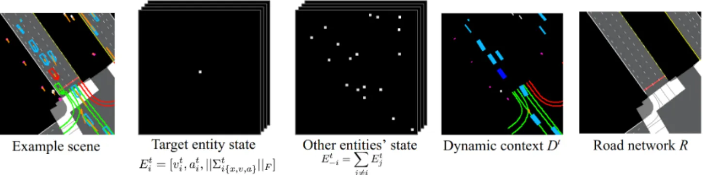
Entity representation We assume access to a black-box perception module which maps from low-level sensor in-formation to 3D tracked entities3_{. For each timestep t,} we have measured quantities for each tracked entityi in-cluding 2D position xt_i, velocity v_it, and acceleration at_i. Our perception module also gives us state estimation uncer-tainty in the form of covariance matrices, and we include this information in our representation via covariance norms ||Σt_i{x,v,a}||F. All feature dimensions are scaled by an esti-mate of their99th_{percentile magnitude to have comparable} dynamic ranges near[−1,1].

We form a tensor for the target entityiat any timestep t denoted Et

i, that has a channel for each state dimsion above, encoding the scalar at the center of the en-tity position, which is in spatial correspondence with road graph tensorR. To model entity interactions, we aggregate all other entities in a tensor encoded in a the same way: E₋t_i=P

j6=iE t

j. These tensors areW×H×7.

Additional dynamic context We encode additional scene context as an RGB imageDt_{of sizeW ×H×3. It contains} oriented bounding boxes for all entities in the scene colored by class type (one of cyclist, vehicle, pedestrian), to encode extents and orientations of objects. It also contains a ren-dering of traffic light permissibility in junctions: we render permitted (green light), yield (unprotected), or prohibited (red light ) by masking road connections in a junction that exhibit each permissibility.

Temporal modelingAll inputs at timesteptand target en-tityiare concatenated (in the third channel dimension) into a tensor:

C_it=hE_it, E₋t_i, Dt, Ri

which isW ×H ×20. See Fig.2for an illustration. We concatenate all Ct

i over past history along a temporal di-mension. We fix the coordinate system for a staticRfor all timestamps by centering the reference frame at the position of the target entity at the time of prediction.

This top-down representation is simple to augment with additional entity features in the future. For example: vehicle brake lights and turn signals, person pose and gestures, and even audio cues could all be integrated as additional state channel dimensions.

3_{This is a reasonable assumption for large companies where such} mod-ules are relatively mature.

Figure 2: Entity and world context representation. For an example scene (visualized left-most), the world is represented with the tensors shown, as described in the text.

(a) One-shot (b) with RNN decoder

Figure 3: Two different network architectures for occupancy grid maps (predicting Gaussian trajectories instead is done by simply replacing the convolutional-transpose network with a fully-connected layer).

3.2. Output representation: modeling uncertainty

and multiple modes

We seek to model an entity’s future states. We believe a good output representation must have the following charac-teristics, which differs from some previous work [10,31]. It should be: (1)A probability distributionover the entity state space at each timestep. The future is inherently uncer-tain, and a single most-likely point estimate isn’t sufficient for a safety-critical system. (2)Multimodal, as it is impor-tant to cover a diversity of possible implicit actions an entity might take (e.g., which way through a junction). (3) One-shot: For efficiency reasons, it is desirable to predict full trajectories (more specifically: time sequences of state dis-tributions) without iteratively applying a recurrence step.

We explore these desiderata by proposing a variety of output distribution representations. The problem can be naturally formulated as a sequence-to-sequence gen-eration problem. For a time instant t, we observe X = {Ct−`+1, Ct−`+2, . . . , Ct} of past scenes, and pre-dict future xy-displacements from time t, denoted Y = {(xt+1, yt+1),(xt+2, yt+2), . . . ,(xt+m, yt+m)}, for a

tar-get entity4_{, where`andmare the time range limits for past} observations and future time horizon we consider. We dis-cuss a variety of approaches to modelP(Y|X)next.

3.3. Parametric regression output with uncertainty

In this representation, we predict sufficient statistics for a bivariate Gaussian for each future position (xt, yt): the mean µt = (µx,t, µy,t), standard deviation σt = (σx,t, σy,t), and spatial correlation scalarρt. This has ben-efits of being a richer and more useful output than vanilla regression. In addition, during learning, the model can at-tenuate the effect of outlier trajectories in the data to have a smaller effect on the loss, an observation made in other problem domains [18].

We train the model to predict log standard deviation st = logσt, as it has a larger numerically-stable range for optimization. We learn parameters via via maximum

likeli-4_{We ignore modeling future entity orientation, but we believe it is} straightforward to extend the ideas here to 3-dof or 6-dof state estimation in future work.

hood estimation logP(Y |X) = t+m X t0_=t+1 logp(xt0, y_t0 |µ_t0, s_t0, ρ_t0), (1)

wherepis the density function of a bivariate Gaussian pa-rameterized byN(µt, σt, ρt).

Multi-modal regression with uncertaintyWe can extend this to predict up to k different Gaussian trajectories, in-dexed by(µi,ˆsi, ρi), and a weightwi associated with the probability of a trajectory, P(Y |X) = k X i=1 wiP(Y |µi,ˆsi, ρi).

However, we run into two major problems with this naive method: (1) exchangeability, and (2) collapse of modes.

For (1), we see that the output is invariant to permu-tations, namely {(µi_{, s}i_{, ρ}i_{)} = {(µ}π(i)_{, s}π(i)_{, ρ}π(i)_{)} for} some permutationπof{1,2, . . . , k}. To illustrate (2), we consider a mixture of two distributions with equal covari-ance, orY ∼ 1

2N(y

1_{, σ}2_{) +} 1 2N(y

2_{, σ}2_{). It can be shown} that ifyi_{are not far enough, specifically|y}1_−y2_|≤2σ[5], then the mixture has a single mode at 1₂(y1_+y2_{), and thus} can be approximated by a single Gaussian parameterized by N(1₂(y1_+y2_{), σ}2₊1

2(y

1_−y2₎2_{). This allows the} learn-ing to center thek Gaussians on a single state with large variance (“mode collapse”), with nothing to encourage the modes to be well-separated.

Inspired by Latent Dirichlet Allocation (LDA) [7], we introduce a latent variablezsuch that(µi, si, ρi)are identi-cally and independently distributed conditioned onz,

P(Y |X) = K X

i=1

P(zi|X)P(Y |µi, si, ρi, zi), (2)

where(µi_{, s}i_{, ρ}i_{)is some fixed function of both the input}

X and latent variablez, resolving the mode exchangeabil-ity problem. To address mode collapse, we choosezto be k-dimensional with small k, and the model is encouraged through the learning procedure to output a diverse set of modes.

To train such a model, we use a conditional variational autoencoder (CVAE) approach, and modelP(z|X)as a cat-egorical distribution, using a Gumbell-Softmax distribution with the reparameterization trick [17] to sample and back-propagate gradients throughz. In our experiments, we use P(z|X)as our discrete, k-Gaussians mixture distribution over state at future timesteps, and refer to this method in our experiments (loosely) as “GMM-CVAE”.

3.4. Non-parametric output distributions

As an alternative to parametric forms, we consider oc-cupancy grid maps [33] as an output representation, where

there is an output grid for each future modeled timestep, and each grid location holds the probability of the correspond-ing output state.

This representation trades off the compactness of the parametric distributions discussed above with arbitrary ex-pressiveness: parametric distributions can capture non-elliptical uncertainty and a variable number of modes at each timestep. Furthermore, they offer alternative ways of integrating into robot planning systems (simple to combine with other non-parametric distributions; fast approximate integration for,e.g., collision risk calculation).

We discretize any future state to 2D grid coordinates

(it, jt). We train a model to maximize log-likelihood on the predicted grid maps gt[i, j] ≡ P(Y = (it, jt)|X), which are discrete distributions over the discretized state space at each timestep. Thus the training loss is a sum of cross-entropy losses fort0∈[t+ 1, t+m].

Diverse Trajectory Sampling: While occupancy maps have intrinsic representational benefits discussed above, it is still useful in many planning applications to extract a dis-crete set of trajectories. We discuss an optimization frame-work to obtain a variable number of trajectories derived from a future occupancy map, with the ability to impose hard and soft constraints on geometric plausibility and di-versity / coverage of the trajectory set.

Letξt = (it, jt)be a sampled discretized state at time

t, andξ ={ξt+1, . . . , ξt+m}be a sampled trajectory. We define a pairwise-structured score for a sampled trajectory as: s(ξ) = t+m X t0_=t+1 logP(Y =ξt0|X)−λ·φ(ξ_t0, ξ_t0₋₁). (3)

whereφ(·,·)can be an arbitrary score function of the com-patibility of consecutive states. We designed a hard-soft constraint cost

φ(ξt, ξt−1) =

(

kξt−v(ξt−1)k2₂ if k·k_∞≤5

∞ otherwise,

whereλ= 0.1was set by hand in our experiments andv(ξt) is the state transitioned to under a constant velocity motion from timettot+ 1. This serves as a Gaussian next-state prior centered on a constant velocity motion model, with a cut-off disallowing unreasonable deviations.

This is an instance of a standard chain graphical model [14], and we can solve for the best trajectoryξ? = arg maxξs(ξ)efficiently using a max-sum message passing dynamic program.

trajec-tories which satisfy: {ξ?1_{, . . . , ξ}?k_{} = arg max} {ξ1_,...,ξk_} k X i=1 s(ξi) (4) subject to: ||ξi−ξj||>1. (5) This seeks to find a set ofktrajectories which maximizes s(·)but are sufficiently far from each other, for some norm || · ||. Following [27], we solve this by iteratively extracting trajectories by solvings(ξ)and then masking regions ofgt to guarantee the distance constraint on the next optimization ofs(ξ)for the next trajectory.

Note this framework is employed only during inference. Incorporating it into a learned end-to-end system is an in-teresting avenue for future work.

3.5. Model

We employ an encoder-decoder architecture for mod-elling, where the encoder maps the 4D input tensor (time ×space×channels) into some internal latent representa-tion, and the decoder uses that representation to model the output distribution over states at a pre-determined set of fu-ture time offsets.

Encoder: We use a convolutional network (CNN) back-bone of 2D convolutions similar to VGG16 [32], on each 3D tensor of the input sequence. Following [3], we found that temporal convolutions acheived better performance and significantly faster training than a recurrent neural network (RNN) structure. To incorporate the temporal dimension, we add in two 3D convolutions – one towards the beginning of the backbone, and one at the end – of kernel size3×3×3

and4×3×3without padding, respectively.

Decoder: We experiment with two different decoding ar-chitectures: (1) “one-shot” prediction of the entire output sequence, and (2) an RNN-decoder which emits a distribu-tion at each inference recurrence step.

One-shot prediction simply requires a two-layer network to regress all the distribution parameters at once, or a 2D convolutional-transpose network with channels equal to the sequence length. For our RNN-decoder, we use only a sin-gle GRU cell, whose hidden output is used to regress the true output, which is then fed in as next input.

For the occupancy grid map output representation, the semantic road map R is fed through a separate, shallow CNN tower (16→ 16→1filters), yielding a spatial grid. This grid intuitively acts as a prior heatmap of static infor-mation that is appended to the decoder before applying soft-max. This should allow the model to easily penalize posi-tions corresponding to obstacles and non-drivable surfaces. See Fig.3for a depiction of the architecture.

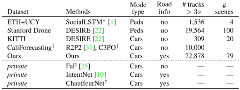
Dataset Methods Mode type Road info # tracks >3s scenes# ETH+UCY SocialLSTM∗_{[1] Peds no 1,536 4} Stanford Drone DESIRE [22] Peds no 19,564 100

KITTI DESIRE [22] Cars no 309 20

CaliForecasting† R2P2 [31], C3PO† Cars no 10,000 —

Ours Ours Cars yes 72,878 79

private FaF [25] Cars no — —

private IntentNet [10] Cars yes — —

private ChauffeurNet† Cars yes — — ∗: Code is publicly available.

†: Method or dataset not yet published.

Table 1: Overview of related public datasets’ training set statistics.

3.6. Implementation Details

Spatio-temporal dimensions: We chose` = 2.5s of past history, and predict up to m = 5s in the future. To re-duce the problem space complexity, we also subsample the past at 2 Hz and predict future control points at 1s inter-vals. We chose the input frames to be 128× 128 pix-els, and chose the corresponding real-world extents to be

50×50m2. The output grid size was set to64×64 pix-els, so that each pixel covers0.78m2. For sampling a di-verse trajectory set, we choose the norm in Equation5 to be||diag([0,1/3,1/3,1/5,1/5])x||∞, in pixel coordinates, which forces greater spatial diversity in later time steps be-tween trajectories.

Model:To conserve memory in our CNN backbone, we use separable 2D convolutions for most of the backbone with stride 2 (see Fig.3). We employ batch-normalization layers to deal with the different dynamic ranges of our input chan-nels (e.g., binary masks, RGB pixel values, m/s, m/s2_). We use CoordConv [23] for all 2D convolutions in the en-coder, which aids in mapping spatial outputs to regressed coordinates. We chose a512-dimensional latent representa-tion as the final layer of the encoder, and for all GRU units.

Training: For training, we started with a learning rate of

10−4 _{and Adam optimizer, and switched to SGD with a} learning rate of 10−5 _{after convergence with Adam. For} training Gaussian parameters we found that pretraining the model on mean-squared error produced better trajectories. All models were trained on a single NVIDIA Maxwell Ti-tan X GPU with Tensorflow Keras. On the dataset described next, training models took approximately 14 hours5_.

4. Experiments

4.1. Dataset

We collected a substantial dataset to evaluate our meth-ods. It is over an order of magnitude larger than [10] and 5_{Training time was heavily dominated by reading data from disk, which} could be significantly optimized with more efficient I/O strategies.

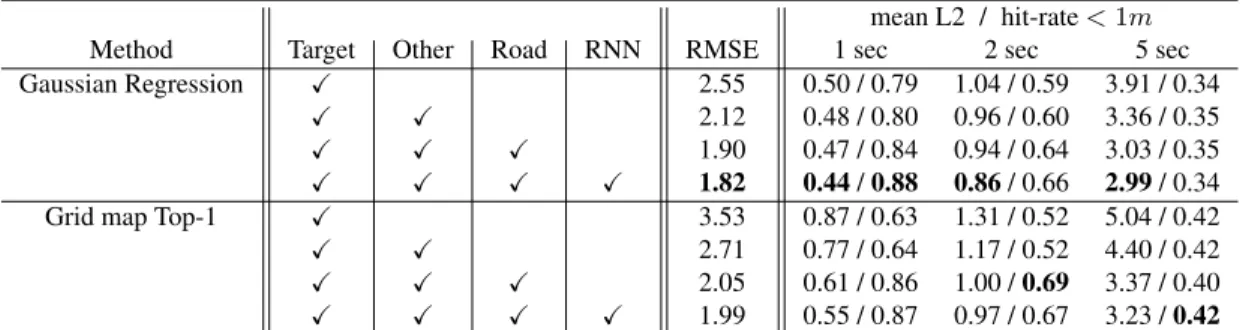
mean L2 / hit-rate<1m

Method Target Other Road RNN RMSE 1 sec 2 sec 5 sec

Gaussian Regression X 2.55 0.50 / 0.79 1.04 / 0.59 3.91 / 0.34

X X 2.12 0.48 / 0.80 0.96 / 0.60 3.36 / 0.35

X X X 1.90 0.47 / 0.84 0.94 / 0.64 3.03 / 0.35

X X X X 1.82 0.44/0.88 0.86/ 0.66 2.99/ 0.34

Grid map Top-1 X 3.53 0.87 / 0.63 1.31 / 0.52 5.04 / 0.42

X X 2.71 0.77 / 0.64 1.17 / 0.52 4.40 / 0.42

X X X 2.05 0.61 / 0.86 1.00 /0.69 3.37 / 0.40

X X X X 1.99 0.55 / 0.87 0.97 / 0.67 3.23 /0.42

Table 2: Ablation study on Gaussian Regression trajectories and Grid Map methods.

Method RMSE 1 sec 2 sec 5 sec

Linear 3.53 0.37/ 0.89 1.08 / 0.62 5.87 / 0.26 Industry 2.31 0.37/0.90 0.92 /0.67 4.18 / 0.40 Gauss. Reg. 1.82 0.44 / 0.88 0.86/ 0.66 2.99/ 0.34 GMM 2.33 0.48 / 0.82 0.95 / 0.65 4.17 / 0.19 Grid map 1.99 0.55 / 0.87 0.97 /0.67 3.23 /0.42 GMM top-5 1.58 0.43 / 0.89 0.79 / 0.70 2.54 / 0.32 Grid top-5 1.25 0.47 / 0.87 0.82 / 0.69 1.39 / 0.56

Table 3: Results for multimodal prediction methods.

many orders of magnitude larger than KITTI [15]. Our dataset consists of tracked vehicles in view of an ego data collection vehicle driving in a dense urban area of San Fran-cisco. A state-of-the-art perception and localization stack processes multiple sensor modalities to produce top-down projected 2D bounding boxes in world coordinates, as well asvt

i,ati andΣti{x,v,a}. We also include the high-definition rendering of the road network, with detailed annotations de-scribed in Section3.1.

The dataset has more than 6.25 million frames from more than173hours of driving in the period of June–July 2018. We split the data into non-overlapping events of7.5

seconds, and extract72,878 train and10,473test events. Events are collected near intersections to skew the dataset distribution towards non-trivial and non-straight driving be-havior. To measure our methods’ generalization power to new intersections, the test/train partition ensures no inter-sections appear in both; there are 79and 9 unique inter-sections in train and test, respectively. To reduce the bias of any one geographic location, we capped the number of samples per intersection at5,000. Note that intersections can be much more complex than simple 4-way junctions.

For an overview of related datasets’ attributes and sizes, please refer to Table1. Note that other vehicle datasets are either quite small (e.g., KITTI [15]), or are not available for comparison. The Stanford Drone dataset is comparable in size and provides a natively top-down representation, which

allows us to extend our model to pedestrian prediction in the future.

4.2. Results

We measure performance of all methods on root mean-squared error (RMSE) over all future timesteps ∆t ∈ {1,2,3,4,5}seconds, as well as the following metrics on 1, 2, 5s futures: (1) L2 distance between the mean predic-tions and ground truth, (2) hit-rate of L2 distance under a

1mthreshold, and (3) oracle error, defined as the minimum L2 distance (i.e.mini

Y −ξi

₂) out of top-kpredictions. Models:We compare the following methods:

· Linear: Baseline that extrapolates trajectories using the most recent velocity and acceleration, held constant. · Industry: Closed-source industry method used in real-world autonomous vehicle driving. It consists of a hybrid of physics, hand-designed rules, and targeted machine learn-ing classification models. Specific problem modes are mod-eled in a custom fashion, requiring multiple person-years of modeling effort.

· Regression with Gaussian Uncertainty: Our method to regress a Gaussian distribution per future timestep.

· Multi-modal Gaussian Regression (GMM-CVAE): Our described method to predict a set of Gaussians, sampling from a categorial latent variable.

· Grid map: Our method to predict occupancy grid maps. To compare to the other methods, we extract trajectories using the described trajectory sampling procedure.

Ablation study:To determine the efficacy of different input channels, we group them and evaluate their performance as follows:

· Target state: State of the entity of interest including its rendered past and present bounding boxes.

· Other state: Features for other dynamic entities including their bounding boxes rendered.

· Road map: Road map and traffic light rendering.

As shown in Table2, each feature type contributes to im-proved model performance: Adding the dynamic context of other entities improves 5s prediction by 0.55m in average

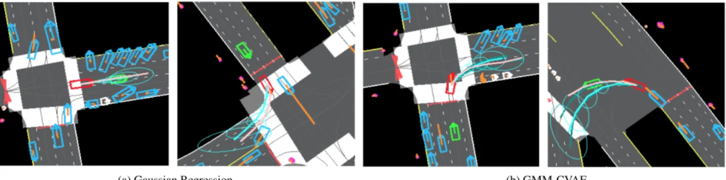
(a) Gaussian Regression (b) GMM-CVAE

Figure 4: Examples of Gaussian Regression and GMM-CVAE methods. Ellipses represent a standard deviation of uncertainty, and are only drawn for the top trajectory; only trajectories with probability>0.05are shown, with cyan the most probable.We see that uncertainty ellipses are larger when turning than straight, and often follow the direction of velocity. In the GMM-CVAE example, different samples result in turning into different lanes in a junction.

Figure 5:Examples of trajectories sampled from the Grid Map method. The rightmost example is a failure case, as the method predicts a mode that turns into oncoming traffic; however, such traffic rules may be hard to discern from only a road map. The method predicts sophisticated behavior such as maneuvering around vehicles and changing lanes.

L2-error, and including the road map adds another 0.33m improvement. See the supplementary material for qualita-tive visualizations of how ablated features contribute to per-formance.

Quantitative method comparison: In Table 3, we com-pare all methods using all features. Evaluating the best-in-top-5 trajectory performed better than the single MAP tra-jectory in all metrics, indicating some value of probabilistic prediction over multiple modes.

In general our mixture of sampled Gaussian trajectories underperformed our other proposed methods; we observed that some samples were implausible. We leave it to future work to determine better techniques for obtaining a diverse set of trajectory samples directly from a learned model.

Interestingly, both Linear and Industry baselines per-formed worse relative to our methods at larger time off-sets, but better better at smaller offsets. This can be at-tributed to the fact that predicting near futures can be ac-curately achieved with classical physics (which both base-lines leverage)—more distant future predictions, however, require more challenging semantic understanding.

Note that while all models are evaluated here in terms of L2-error, none of the models directly optimize this

quan-tity but instead optimize the likelihood of distributions over the future state space, which has other benefits over regression—this is demonstrated in the top-5 metric, as well as in the qualitative results below.

Qualitative Analysis: We show examples of the Gaus-sian Regression and GMM-CVAE trajectories in Fig.4, and sampled Grid Map trajectories in Fig. 5. Please see the supplementary material for more examples and visualiza-tions. Overall, trajectories have plausibly learned traffic rules: lane-keeping, traffic light obeyance, following behav-ior, and even the illegal ones are specious.

5. Conclusion

We present a unified framework for multimodal future state prediction. Our novel input encoding encapsulates static and dynamic scene context, taking advantage of mea-surements from sensor modalities and a high-definition road map. We experiment with continuous and discrete output representations, and arrive at solutions that address the un-certainty and multi-modality of future prediction. Empirical and qualitative evaluation show that our methods improve on baselines that do not encode scene context, and success-fully create diverse samples in complex driving scenarios.

References

[1] A. Alahi, K. Goel, V. Ramanathan, A. Robicquet, L. Fei-Fei, and S. Savarese. SocialLSTM: Human trajectory prediction in crowded spaces.CVPR, 2016.2,6

[2] T. M. Bagautdinov, A. Alahi, F. Fleuret, P. Fua, and S. Savarese. Social scene understanding: End-to-end multi-person action localization and collective activity recognition. InCVPR, 2017.2

[3] S. Bai, J. Z. Kolter, and V. Koltun. An empirical evaluation of generic convolutional and recurrent networks for sequence modeling.arXiv:1803.01271, 2018.6

[4] M. Bansal, A. Krizhevsky, and A. Ogale. Chauffeurnet: Learning to drive by imitating the best and synthesizing the worst.arXiv preprint arXiv:1812.03079. 2,3

[5] J. Behboodian. On the modes of a mixture of two normal distributions.Technometrics, pages 131–139, 1970.5

[6] A. Bhattacharyya, M. Fritz, and B. Schiele. Long-term on-board prediction of people in traffic scenes under uncertainty. InCVPR, 2018.2

[7] D. M. Blei, A. Y. Ng, and M. I. Jordan. Latent dirichlet allocation.JMLR, 2003.5

[8] M. Bojarski, D. Del Testa, D. Dworakowski, B. Firner, B. Flepp, P. Goyal, L. D. Jackel, M. Monfort, U. Muller, J. Zhang, et al. End to end learning for self-driving cars. arXiv preprint arXiv:1604.07316, 2016.2

[9] S. Bullinger, C. Bodensteiner, M. Arens, and R. Stiefelha-gen. 3d vehicle trajectory reconstruction in monocular video data using environment structure constraints. In ECCV, 2018.1

[10] S. Casas, W. Luo, and R. Urtasun. Intentnet: Learning to predict intention from raw sensor data. InCoRL, 2018.2,3,

4,6,7

[11] C. Chen, A. Seff, A. Kornhauser, and J. Xiao. Deepdriving: Learning affordance for direct perception in autonomous driving. InICCV, 2015.2

[12] X. Chen, H. Ma, J. Wan, B. Li, and T. Xia. Multi-view 3d object detection network for autonomous driving. InCVPR, 2017.1

[13] N. Dinesh Reddy, M. Vo, and S. G. Narasimhan. Carfusion: Combining point tracking and part detection for dynamic 3d reconstruction of vehicles. InCVPR, 2018.1

[14] P. F. Felzenszwalb and D. P. Huttenlocher. Pictorial struc-tures for object recognition.IJCV, 61(1):55–79, 2005.5

[15] A. Geiger, P. Lenz, and R. Urtasun. Are we ready for au-tonomous driving? the kitti vision benchmark suite. CVPR, 2012.1,2,7

[16] B. Ivanovic, E. Schmerling, K. Leung, and M. Pavone. Generative modeling of multimodal multi-human behavior. 2018.2

[17] E. Jang, S. Gu, and B. Poole. Categorical reparameterization with gumbel-softmax.ICLR, 2017.5

[18] A. Kendall and Y. Gal. What uncertainties do we need in bayesian deep learning for computer vision?NIPS, 2017.4

[19] K. M. Kitani, B. D. Ziebart, J. A. Bagnell, and M. Hebert. Activity forecasting.ECCV, 2012.2

[20] Y. Kong and Y. Fu. Human action recognition and prediction: A survey.arXiv preprint arXiv:1806.11230, 2018.2

[21] J. F. P. Kooij, N. Schneider, F. Flohr, and D. Gavrila. Context-based pedestrian path prediction. InECCV, 2014.

2

[22] N. Lee, W. Choi, P. Vernaza, C. B. Choy, P. H. S. Torr, and M. K. Chandraker. DESIRE: distant future prediction in dy-namic scenes with interacting agents. CVPR, 2017. 1,2,3,

6

[23] R. Liu, J. Lehman, P. Molino, F. P. Such, E. Frank, A. Sergeev, and J. Yosinski. An intriguing failing of convo-lutional neural networks and the CoordConv solution. arXiv preprint arXiv:1807.03247, 2018.6

[24] W. Lotter, G. Kreiman, and D. D. Cox. Deep predictive cod-ing networks for video prediction and unsupervised learncod-ing. CoRR, 2016.2

[25] W. Luo, B. Yang, and R. Urtasun. Fast and furious: Real time end-to-end 3d detection, tracking and motion forecast-ing with a sforecast-ingle convolutional net.CVPR, 2018.1,2,6

[26] A. Mousavian, D. Anguelov, J. Flynn, and J. Koˇseck´a. 3d bounding box estimation using deep learning and geometry. InCVPR, 2017.1

[27] D. Park and D. Ramanan. N-best maximal decoders for part models.ICCV, 2011.6

[28] D. A. Pomerleau. Alvinn: An autonomous land vehicle in a neural network. InNIPS, 1989.2

[29] C. R. Qi, H. Su, K. Mo, and L. J. Guibas. Pointnet: Deep learning on point sets for 3d classification and segmentation. CoRR, 2016.1

[30] N. Rhinehart and K. M. Kitani. First-person activity fore-casting with online inverse reinforcement learning. InICCV, 2017.2

[31] N. Rhinehart, K. M. Kitani, and P. Vernaza. R2p2: A repa-rameterized pushforward policy for diverse, precise genera-tive path forecasting.ECCV, 2018.2,3,4,6

[32] K. Simonyan and A. Zisserman. Very deep convolutional networks for large-scale image recognition.CoRR, 2014.6

[33] S. Thrun, W. Burgard, and D. Fox. Probabilistic Robotics. MIT Press, 2005.5

[34] J. Wiest, M. Hoffken, U. Kresel, and K. Dietmayer. Prob-abilistic trajectory prediction with gaussian mixture models. Intelligent Vehicles Symposium, 2012.2

[35] Y. Zhou and O. Tuzel. VoxelNet: End-to-end learning for point cloud based 3d object detection.CoRR, 2017.1