A Quantitative Assessment of the Decline in the U.S. Saving Rate

A Quantitative Assessment of the Decline in the U.S. Saving

Rate

Kaiji Cheny _{Ay¸se ·Imrohoro¼glu}z _{Selahattin ·Imrohoro¼glu}z

First Version October 2005; this Version December 2007

Abstract

The saving rate in the U.S. has been declining since 1960s. There have also been sig-ni…cant secular changes in population growth, tax rates on labor and capital income, and the depreciation rate of capital in this period. We use the standard growth theory cali-brated to the U.S. data to evaluate the quantitative role of these factors in contributing to the decline in the saving rate. Our …ndings indicate that the decline in the population growth rate and the increase in the depreciation rate are signi…cant in explaining the secular trends, where as the medium term ‡uctuations in the total factor productivity seem important in driving the year-to-year movements in the U.S. saving rate since the 1960s.

Department of Economics, University of Oslo

z_{Department of Finance and Business Economics, Marshall School of Business,}

Uni-versity of Southern California, Los Angeles, CA 90089-1427.

We would like to thank the seminar participants at USC, University of California at Riverside, Federal Reserve Bank of Chicago, Conference on Economic Dynamics at the University of Tokyo, 2006 Annual Meet-ings of the Society for Economic Dynamics, CEMFI, Madrid, IIES, Stockholm University, Indiana University, Purdue University, and CERGE-EI, Charles University in Prague for helpful comments.

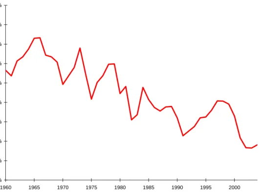
2% 4% 6% 8% 10% 12% 14% 16% 18% 20% 1960 1965 1970 1975 1980 1985 1990 1995 2000 Saving Rate

Figure 1: Net National Saving Rate in the U.S.

1

Introduction

The net national saving rate in the U.S. displayed in 1, has declined from an average of 15% in 1960s to 10% in 1980s and 8.6% in 1990s.

This secular decline has occupied center stage in policy discussions and continues to attract media coverage. Understanding this decline as well as the di¤erences in saving rates across countries has also been an important part of academic research. Detailed data analyses have been conducted to explore whether particular cohorts are responsible for the low saving rate by examining personal saving rates in the U.S. For example, Gokhale, Kotliko¤, and Sabelhaus (1996) attribute the decline in the saving rate to the redistribution of resources through social security and medicare, from young consumers with low marginal propensities to consume, to older generations with high marginal propensities to consume. Attanasio (1998) argues that cohorts born between 1925 and 1939 may be to blame for the low personal saving rate. Summers and Carroll (1987) suggest that it is the reliance of the younger generations on social security that depresses saving in the U.S. Boskin and Lau (1988a,b) formulate a model based on longitudinal and cross-sectional microeconomic data together with aggregate time series and examine the importance of various factors a¤ecting aggregate consumption and saving in the U.S. Their results suggest that it is the decline in the saving

of generations born after the great depression that may be responsible for the decline in the national saving rate. Summers, Carroll and Blinder (1987) examine the decline in the national saving rate and conclude that it has been due to a combination of federal de…cits and a continuation of a long term trend in private savings.1

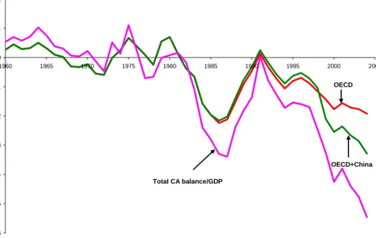
Another notable change during this time period has been the growing current account de…cit in the U.S. Figure??displays the CA de…cit between the U.S. and a set of its trading partners between 1960 and 2004. The secular decline in the current account especially since the 1990s is evident in all the series.2 _{Several authors have been analyzing the reasons}

for these large global imbalances such as Backus, Henriksen, Lambert and Telmer (2005), Bernanke (2005), Fogli and Perri (2006), Gourinchas and Rey (2005), Henriksen (2006), Mendoza, Quadrini and Rios-Rull (2007), Obstfeld and Rogo¤ (2004), Roubini and Setser (2005), Summers (2004).

Since 1960s there have been substantial changes in several variables in the U.S. that can have potentially important consequences for the behavior of the national saving rate and the current account balances. Between 1960 and 1980 the average population growth rate and the depreciation rate were 1.8% and 4.3%, respectively. By 2000 the population growth rate had declined to about 0% while the depreciation rate had increased to 5.3%.3 Each of these changes would reduce the demand for investment in the Solow growth model. While both of these changes would put a downward pressure on the saving rate in the U.S., there were other changes in the economic environment, such as the decline in the capital income tax rate, that would have encouraged savings over this time period. Meanwhile some of these exogenous variables have been changing at di¤erent rates in the rest of the world.

In this paper we explore the quantitative implications of the changes in these and some other economic factors on the secular trends in the net national saving rate and the current account balance using standard growth theory.4 In particular, we use a two country

1_{Another set of papers have focused on the possible relationship between the increase in stock prices and the} boom in consumer spending. For example, see Parker (1999) and Juster, Lupton, Smith, and Sta¤ord (2000) who suggest that the signi…cant capital gains in corporate equities experienced since 1984 is responsible for the decline in the personal saving rate. Backus, Henriksen, Lambert, and Telmer (2005) argue that private saving rates are strongly and negatively correlated with the ratio of net worth to consumption. Also see Poterba (2000) for a survey.

2_{Data on U.S. current account balance against various regions come from International Economic Accounts} of Bureau of Economic. The data on U.S. current account balance against our sample of OECD countries are the sum of U.S. current account balance against Western Europe, Canada and Japan. Since 1999 we use the U.S. current account balance against EU-15 to substitute for U.S. current account balance against Western Europe.

3_{Gomme and Rupert (2005) provide detailed calculations for the depreciation rate of di¤erent types of} capital. Their …ndings also indicate increasing depreciation rates since 1960s.

4

CA Balance/GDP -0.06 -0.05 -0.04 -0.03 -0.02 -0.01 0 0.01 0.02 1960 1965 1970 1975 1980 1985 1990 1995 2000 2005 Total CA balance/GDP OECD OECD+China

Figure 2: U.S. Current Account De…cit

neoclassical growth model with an in…nitely-lived representative agent facing complete mar-kets. We calibrate the economy to the U.S. data for the 1960-2004 period. For the second country we restrict our attention to the OECD countries and calibrate their TFP growth rate, population growth rate and tax rates for the same period. Our exogenous driving forces are the population growth rate, tax rates on capital and labor income, share of government expenditures in output, depreciation rate, and actual time series data for the TFP growth rate. We conduct deterministic simulations, as in Hayashi and Prescott (2002), and perform an ‘accounting exercise’to evaluate the impact of several factors that may explain the secular trends in the saving rate and the current account.

We …nd that the model generated saving rate, consumption and capital resemble the data reasonably well until the 1990s. The model generated saving rate declines from an average of 17% in 1960s to about 8% by 1990. Our results suggest that the decline in the population growth rate and the increase in the depreciation rate alone account for 3-4 percentage point decline in the saving rate by early 1990s. Changes in the TFP growth rate generate annual ‡uctuations in the saving rate that resemble the data reasonably well but do not contribute

In particular, we follow the methodology of Cole and Ohanian (1999, 2002, 2004), Kehoe and Prescott (2002), and Chen, ·Imrohoro¼glu and ·Imrohoro¼glu (2006a) in using an applied general equilibrium setup to account for the observed time path of the U.S. saving behavior.

to the secular decline in the saving rate. Our results indicate that the di¤erences in the TFP growth rates of the U.S. and the OECD countries contributed signi…cantly to the growing current account imbalances between them.

The paper is organized as follows. Section 2 presents the growth model we use to evaluate the models’s implications for the closed and the open economies. Data and calibration issues are discussed in Section 3, quantitative …ndings and the sensitivity analysis are presented in Section 4. Concluding remarks are given in Section 5. Appendix A contains calibration details and data sources.

2

A Two-Country Model

Consider a standard perfect foresight two-country growth economy. For each country i = f1;2_g;there is a stand-in household with Ni

t working-age members at datet. Both capital

and labor are immobile across countries. We assume that there is a risk-free bond traded internationally each period. The size of the household evolves over time exogenously. In this framework a representative household maximizes

1 X t=0 t_Ni t(logcit+ log(1 hit)) subject to B_ti₊₁+C_ti+X_ti+ K_ti X i t Ki t 'i gi 1 1 _ni _{1 +} i 2 B_ti 1 +r_tB + 1 i_h;t w_tiH_ti+ri_tK_ti i_kt(r_ti i_t)K_ti+T Ri_t i_t (1) K_ti₊₁ = 1 i_t K_ti+X_ti (2) B₀i; K₀i given,

where ci_t=C_ti=N_ti is per member consumption, hi_t=H_ti=N_ti is the fraction of hours worked per member of the household, is the subjective discount factor, is the share of leisure in the utility function, H_tiis total hours worked by all working-age members of the household,

i

h;t and ik;t are tax rates on labor and capital income, respectively, at timet; witis the real

wage,T Ri_tis a government transfer, i_tis a lump sum tax,ri_tis the rental rate of capital, and

i

t is the time-tdepreciation rate in country i. The size of the household evolves over time

exogenously at the rateni_t=N_ti=N_ti ₁: 'i = gi 1

1 _ni ₁₊ i_{which is the investment capital}

ratio at the steady state. Following the literature we have added quadratic adjustment costs for each countries’ capital accumulation represented by Ki

t Xi t Ki t 'i 2_{; where g}i_{; n}i _and i _{denote the value of their counterparts on the balanced growth path.}5

5

By setting = 0we examine the role of this assumption on the model generated current account balances. In general, adjustment costs cause the current account from ‡uctuating too much. They have no signi…cant impact on the secular patterns we …nd.

Households are assumed to own the capital, K_ti; and rent it to businesses. The law of motion for the capital stock is given by 2:

The aggregate production function is given by

Y_ti=A K_ti (H_ti)1 ;

where is the income share of capital and At is total factor productivity, which grows

exogenously at the rate gi

t=Ait=Ait 1.

2.1 Government

For each country i, there is a government that taxes income from labor and capital (net of depreciation) and uses the proceeds to …nance exogenous streams of government purchases

Gi_tand government transfers T Ri_t:A lump sum tax i_tis used to ensure that the government budget constraint is satis…ed each period:

Gi_t+T Ri_t= i_h;tw_tiH_ti+ i_k;t(r_ti i_t)K_ti+ i_t:

In other words, i_t is the primary government de…cit in the model. National account identity is given by:.

C_ti+I_ti+Gi_t+B_ti₊₁ =Y_ti+B_ti 1 +r_tB :

or

C_ti+I_ti+Gi_t+CAi_t=Y_ti+B_tir_tB=GN P_ti

whereCAi

t=Bit+1 Btiis the current account balance for countryi; Iti =Xti+ Kti Xi

t

Kti

'i 2_:

2.2 Competitive Equilibrium

Given government policy _fGi_t; T Ri_t; i_h;t; _k;ti ; i_tg1_t=0, fori = 1;2, a competitive equilibrium consists of allocations _fC_ti; I_ti; H_ti; K_ti₊₁; Y_ti; B_ti_g1_t=0 and prices _fwi_t; r_ti; r_tB_g for i= 1;2, such that

given policy and prices, the allocation solves the household’s problem in each i,

given policy and prices, the allocation solves the …rm’s pro…t maximization problem with factor prices given by: wi_t= (1 )Ai_t K_ti (H_ti) ;andr_ti = Ai_t K_ti 1(H_ti)1 ;

the government budgets are satis…ed,

the goods market clears for each country: C_ti+I_ti +Gi_t+N X_ti =Y_ti; where N X_ti =

CAi

t BtirtB is the net export for country i:

This environment can be turned into a closed economy model by shutting down the international bond market. In fact we will start with the closed economy model to investigate the decline in the saving rate in the U.S. Later we will allow for free trade to understand the implications of the model on the current account.

2.3 Numerical Solution

Equilibrium Conditions: For each country, the equilibrium conditions of this model can be described in three equations below:

hi_t 1 hi t = (1 i_h;t)(1 )Y i t Ci t ; (3) q_ti = 1 + 2 X i t K_ti ' i ₍₄₎ qi_tC i t+1 N_ti₊₁ = C_ti N_ti 8 < : q_ti₊₁ 1 i_t+1 + (1 _k;ti ₊₁) Ai_t+1(K_ti₊₁) 1(H_ti₊₁)1 i_t+1 + i_t+1 Xi t+1 Ki t+1 'i + 2 X i t+1 Ki t+1 Xi t+1 Ki t+1 'i 9 = ;(5); C_ti₊₁ N_ti₊₁ = C_ti N_ti 1 +r B t+1 (6) I_ti = X_ti+ K_ti X i t Ki t 'i 2 (7) I_ti = Ai_t(K_ti) (Ht)1 Cti Git Bti+1 1 +rtB Bti : (8) where qt is Tobin’sq:

Detrending: For an aggregate variable of each country i, denoted as zi_t; its detrended version is given by: z_eti=Z_ti=h Ai_t

1

1 _Ni

t

i

:Note that for each country, an aggregate variable is detrended by its own TFP factors and population size. Applying this change of variables

to(3);(5)and (??), we obtain equations qt = 1 + 2 e xi_t+1 e ki t+1 'i ! (9) qtecit+1 = e ci_t g_ti₊₁ 1 1 8 > > < > > : qt+1 1 it+1 + (1 k;ti +1) ekit=hit 1 i t+1 + it+1 e xi t+1 e ki t+1 'i _{+ 2} xeit+1 e ki t+1 e xi t+1 e ki t+1 'i 9 > > = > > ; ; (10) e ci_t+1 = ec i t g_ti₊₁ 1 1 1 +r_tB₊₁ (11) eii_t = x_eti+ ek_ti₊₁ xe i t+1 e k_ti₊₁ ' i !2 (12) eii_t = (1 i_t) eki_t hi_t 1 (13) e ci_t ebi_t+1 g_ti₊₁ 1 1 _ni t+1 1 +rtB ebit ; (14)

where _tis the ratio of government purchases to output,Gi

t=Yti:The detrended international

bond market clearing equation is

eb1_t+1= eb2_t+1st+1 (15)

where we follow McGrattan and Prescott (2007) and denote st+1 =

A2 t+1 A1 t+1 1 1 N2 t+1 N1 t+1 as the relative size of the two countries. Note that we can solve recursively for the whole sequence

of st+1 byst+1=st g2 t+1 g1 t+1 1 1 n2 t+1 n1 t+1

;given s0 and the whole sequence of git; nit i=1;2:

Transition to the steady-state: Starting from a given initial asset distribution K₀1; K₀2; B₀1; B₀1

we compute the saving rate using

sav_ti = GN P i t Git Cti itKti GN Pi t itKti :

and we can compute the current account de…cit as a percentage of GDP as

cai_t= B

i

t+1 Bti

Y_ti

Algorithm: Note that in this perfect foresight two country economy, given the steady state net foreign asset distribution neb1;eb2o, we can solve for other macro variables in the steady state. However, the steady state net foreign asset distribution depends critically on the transition path and the initial asset distribution.6 Therefore we need to solve for the

6_{As Chattejee (1994) shows in a complete market economy there are in…nite number of steady state wealth} distributions.

transition path and the steady state simultaneously. Note also for equations(10)and(11)to hold for each country at the steady state, it must be g1 =g2 at the steady state. Similarly, for the relative size of the country to be stationary, we have n1=n2:

We assume that the economy reaches steady state at some future date T: Then start-ing from some initial asset distribution nek1

0;ek20;eb10;eb20

o

; we can solve for the whole path

of n_ec1_t;_ec2_t; rB_t ;ek1_t+1;ek_t2₊₁;eb1_t+1;eb2_t+1; h1_t; h2_to T_t=0 using the systems of nonlinear equations(3), (10);(11);(13) and(15):To rule out Ponzi schemes, we require that at the steady state

ebi_T+1 gi_T 1 1 _ni T 1 +rBT = (1 iT) ekTi hiT 1 e ci_T x_ei_t

so that agent will not borrow in…nitely. Note however, it is possible that at steady state

ebi ₆= 0:

3

Calibration

Our analysis is limited by the number of countries for which we can get consistent estimates of several exogenous variables, in particular the TFP growth rate. Consequently, we restrict our analysis to the CA balance between the U.S. and the OECD countries.7 We calibrate model economy using data from Groningen Total Economy Database.8 _{We derive TFP}

growth rates for the U.S. and the OECD countries using the Solow decomposition.9 We also compute the average population growth rate of the OECD using the same weighting method.

Constant Parameters: There are 3 parameters that are time and country invariant throughout our analysis. The capital share parameter, ;is set to0:4. The capital adjustment cost parameter, , is set to 1, which is well within the range of values used in the literature.10

7

More speci…cally, our sample OECD countries include Austria, Canada, Belgium, Denmak, Finland, France, Germany, Greece, Iceland, Ireland, Italy, Japan, Netherland, Norway, Portugal, Spain, Sweden, Switzerland, United Kingdoms.

8_{The data on the capital stock is not available from Groningen Total Economy Database. To compute} the real capital stock that is consistent with real GDP in constant 1990 dollars (converted at Geary Khamis PPPs), we collect the data of real total capital stock as a percentage of real GDP between 1960 and 2001 from the Kiel Institute database on Capital stock in the OECD countries. We then multiply this ratio with real GDP from Groningen Total Economy Database to obtain data of real capital stock for each country. We impute the real capital stock after 2001 by multiplying the real total capital stock as a percentage of real GDP at 2001 and the real GDP in each of the last three years.

9

For the OECD, we generate aggregate output, capital, and hours as the weighted sum of each individual country’s output, capital and hours, all weighted by each individual country’s output share. Then we use the Solow decompsition to get aggregate TFP for the OECD. The TFP computed in this way di¤ers very little from the TFP computed as the weighted average of TFP of individual countries, weighted by each country’s output share.

1 0

The subjective discount factor, ; is set to 0:9702so that the capital output ratio is 3:2 at the …nal steady state. The share of leisure in the utility function, ;is set to1:45 to match an average workweek of 35 hours. These choices are summarized below.

Time-Invariant Parameters 0:4 1960-2004 average

0:9702 Target: K=Y = 3:3in steady state 1:45 Target: Average workweek = 35hours

Calibration of 2005 and beyond and the Steady-State: We assume that the U.S. and the OECD start from given conditions in 1960 and eventually converge to a steady-state in 2070. In our benchmark model, we set the seven exogenous variables in the below table equal to their steady state values starting in 2005.11 _{Note that the population growth}

rate in the U.S. has been declining since the 1960s and according to the Census Bureau projections it will continue at very low rates in the future. Based on the "middle" growth projections by the Census Bureau’s we set the population growth rate after 2004 and at the steady state equal to 1%: Since projections for the OECD countries are not very di¤erent from the U.S. we set the steady state population growth in the OECD also equal to 1%.12

Similarly, the depreciation rate has been increasing in the U.S. For the periods after 2004 and at the steady state, we set the depreciation rate equal to 5%which is the depreciation rate in 2004.13 Our results are not sensitive to di¤erent assumptions about the calibration of most of the variables for the period 2005 and beyond. One variable that matters for the results is the growth rate of TFP. We discuss its impact in the sensitivity analysis.

1 1

With our assumed tax rates, the government budget will be in a surplus at the steady state. 1 2

Population growth rates are the growth rates of civilian non-institutional population 16 years and over reported by the BLS. Population projections are taken from U.S. Bureau of the Census (http://www.mnforsustain.org/united_states_population_growth_graph.htm)

1 3

Gomme and Rupert (2005) provide detailed calculations for the depreciation rate of di¤erent types of capital. Increasing depreciation rates are evident in computers and to some extent in market structures since 1960s. For the OECD countries we use the same depreciation rates as the U.S.

Steady-State Values: 2005 and Beyond

U.S. OECD

gt 1 TFP Growth Rate 0.011 0.011

nt 1 Population Growth Rate 0.01 0.01

t Government Purchases to GDP Ratio 0.16 0.18

t Depreciation Rate 0.05 0.05

T Rt=GDP Transfers to GDP Ratio 0.08 0.08 k;t Capital Income Tax Rate 0.42 0.34 h;t Labor Income Tax Rate 0.29 0.38

Calibration of the 1960-2004 period: In our benchmark simulation, we use the actual time series data between 1960-2004 for the TFP growth rate, gt 1;population growth rate,

nt 1;depreciation rate, ;share of government purchases inGDP, t;share of government

transfers inGDP,T Rt=GDPt;and capital and labor income tax rates, k;t; h;t.14 Empirical

marginal tax rates for the U.S. are constructed using the methods of Joines (1981) and McGrattan (1994). The tax rate data for foreign country comes from updated calculations of Mendoza, Teasar and Razin (1996) up to 1996. For years after 1996, the tax rate are the same as those of 1996. The data used in the calibration are provided in the Appendix. We use the initial capital-output ratio for the U.S. in 1960, 3:5; to pin down, ek₁₉₆₀1 ; the initial capital stock for the home country. We set the initial capital stock for the foreign country,

e

k2₁₉₆₀, to be 1.55 times ek₁₉₆₀1 ;which is the actual ratio of capital stock between OECD and the U.S. in 1960. The initial foreign asset holdings,eb1

1960 andeb21960 are both set to be zero.

A very important variable for the results is the size of the U.S. relative to the OECD countries in 1960. This relative size determines the importance of the U.S. in shaping the world prices relative to the OECD. If the OECD is too small to impact the world prices then the model converges to the closed economy case with a zero current account balance for the U.S. As we change the initial relative size, to make the OECD countries matter more and more in 1960, our current account surplus for the U.S. in 1960s and the current account de…cit in 2004 get larger and larger. In our benchmark calibration. we have chosen the relative size such that the current account de…cit generated by the model in 1960 is not too far o¤ from the data. After the initial size is pinned down, the actual TFP and population growth rates determine the evolution of the relative size over time. 15

1 4_{The data on government purchases as a percent of GDP is calculated using the data of Government …nal} consumption expenditures in national currency units for each country from OECD annual national accounts. Data on transfer for the U.S. is obtained from National Income and Product Acocunts. We use the same data for the OECD countries. We obtain data on population from 15-64 years old from UN demographic year book (1960-1969) and OECD Economic Outlook (1970-2005).

1 5

4

Results

We start this section by presenting the properties of the closed economy and focus on the secular trends in the saving rate between 1960 and 2004. We show that the standard neo-classical model can be an e¤ective tool in understanding the behavior of the saving rate until the early 1990s..16 In the second section we discuss the model predictions with respect to the current account balance between the U.S. and the OECD countries.

4.1 Properties of the model-Closed Economy

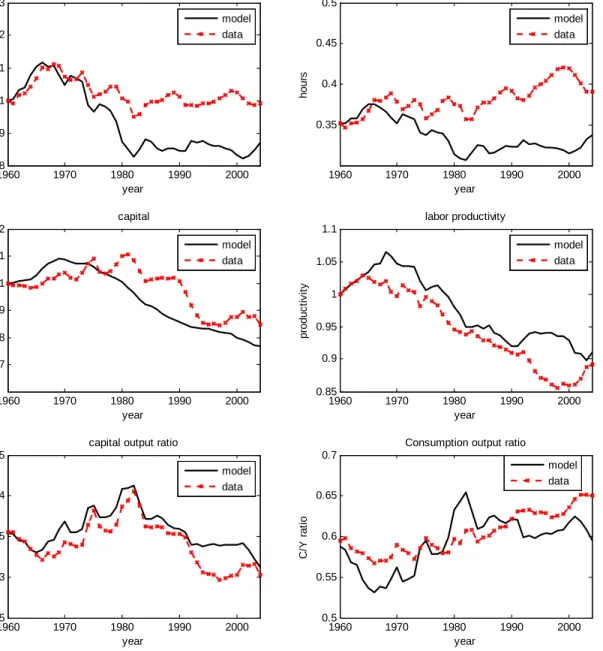
Figure 3 displays the model’s predictions for per capita GNP, hours, capital, labor produc-tivity, capital output ratio and consumption output ratio together with their counterparts in the data. The model generated series and the data, except for hours per capita, are all detrended by 1.018t.

The model generated hours per capita and GNP per person in Figure 3 display large gaps from their counterparts in the data. These discrepancies were noted by other authors, such as Uhlig (2003) and McGrattan and Prescott (2007). Notice that the model generated hours per capita displays a decline while hours per capita in the data increase. The reason for the hours boom in the U.S. is not well established. One possibility is the increase in the labor force participation of women. McGrattan and Rogerson (2004) show that the increase in hours per capita observed in the U.S. is mainly due to the increase in the labor force participation rate of females. In fact, between 1950 and 2000, employment to population ratio of women increases by 87% while that of men declines by 15.7%. Between 1980 and 2000 employment to population ratio of women increases by 17%. The simple framework used in this model is not capable of mimicking these trends.17 It is also possible that the reason for the hours boom lies somewhere else such as the intangible capital explanation being advanced by McGrattan and Prescott (2007) or the change in wage markups argued by Smets and Wouters (2007).

In order to further understand the performance of the standard model, but without taking a stand on the main reasons behind the hours boom in the data, we introduce a labor wedge into the model. We would get a perfect match between the model and the data if we introduced a labor wedge and an investment wedge that would force equations (1) and (2)

the role of the U.S. in shaping the world prices. 1 6

For a closed economy the calibration is slightly di¤erent since it is done over GNP instead of GDP. The details of this calibration are explained in the Appendix. We also set the adjustment costs equal to zero for the closed economy experiments.

1 7_{Several papers investigate the rise of the female labor force participation such as Jones, Manuelli and} McGrattan (2003), Olivetti (2001), Akbulut (2005), and Caucutt, Guner, and Knowles (2002).

1960 1970 1980 1990 2000 0.8 0.9 1 1.1 1.2 1.3 GNP per person year GNP per pers on 1960 1970 1980 1990 2000 0.35 0.4 0.45 0.5

hours per capita

year hours 1960 1970 1980 1990 2000 0.7 0.8 0.9 1 1.1 1.2 capital year c api tal 1960 1970 1980 1990 2000 0.85 0.9 0.95 1 1.05 1.1 labor productivity year produc ti v it y 1960 1970 1980 1990 2000 2.5 3 3.5 4 4.5

capital output ratio

year K/Y r a ti o 1960 1970 1980 1990 2000 0.5 0.55 0.6 0.65 0.7

Consumption output ratio

year C /Y r a ti o model data model data model data model data model data model data

to hold. In the following experiment we introduce only the labor wedge to examine the role of labor in generating the results in Figure 1. Speci…cally we use the labor wedge calculated from

Lwt=

htCt

(1 ht)(1 h;t)(1 )Yt

:

After computing the labor wedge we replace (1 h;t) in (1) with (1 h;t)Lwt: Since

we already have taxes in this model, the labor wedge would have to be a proxy for labor distortions other than taxes.

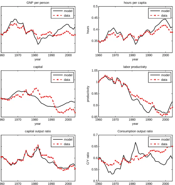
Figure 4 displays the results of this experiment with the labor wedge. Hours per capita do not match the data perfectly since we only have the labor wedge and do not have the investment wedge. The rest of the model generated series resemble the U.S. data reasonably well. We conjecture that extensions of the standard model which can capture the hours boom will be successful in mimicking the other aspects of the U.S. economy well.18

In Figure 5 we display the data and the model generated net national saving rate with and without the labor wedge between 1960 and 2004. Saving rates generated by the two models are remarkably similar to each other until late 1980s. They both capture the secular decline between 1960 and early 1980s, as well as the annual ‡uctuations in the actual U.S. data. However, both models generate higher saving rates than in the data for the 1960s and lower rates for 1980.19 After mid 1980s the model with the labor wedge predicts higher saving rates than the model without the wedge. The di¤erences in the saving rates between the two models grow in the 1990s. While the saving rate generated by the model without the labor wedge seems to mimic the data well for 1990s, we don’t consider it a successful model since its performance along other dimensions as shown in Figure 1 are not satisfactory. However, the …nding that the saving rates generated by the two models are "similar" until the 1990s indicates that the model without the labor wedge is reasonably good in replicating the consumption-invesment trade-o¤ in the actual economy for that period even though it misses the consumption leisure trade-o¤. Consequently, we will rely on the standard model to further examine the factors behind the secular decline in the saving rate until 1990s.

1 8

The labor wedge needed to generate these results is not non-negligible especially for the 1984-2004 period. It starts at the value of 1.0 in 1960 and grows to 1.12 at the end of 1984. However, the wedge that is needed to match the hours has to increase by 42% between 1984 and 2004. It is hard to explain the size of the wedge using labor distortions other than taxes especially for the later period. For the earlier period, it is possible that a model which incorporates the increases in labor force participation of women may explain the size of the wedge needed.

1 9_{Later in sensitivity analysis, we show that some of the large ‡uctuations obtained in these graphs are due} to the perfect foresight assumption. When TFP growth rate is assumed to be stochastic, the simulated saving rates display smaller ‡uctuations compared to the perfect foresight case. Households’intertemporal behavior is subdued due to the lack of perfect foresight of the real return to capital. None of the other features of the analysis change signi…cantly when the perfect foresight assumption is abandoned. This is consistent with the …ndings in McGrattan and Prescott (2007).

1960 1970 1980 1990 2000 0.8 0.9 1 1.1 1.2 1.3 GNP per person year GNP per pers on 1960 1970 1980 1990 2000 0.35 0.4 0.45 0.5

hours per capita

year hours 1960 1970 1980 1990 2000 0.8 0.9 1 1.1 1.2 1.3 capital year c api tal 1960 1970 1980 1990 2000 0.85 0.9 0.95 1 1.05 labor productivity year produc ti v it y 1960 1970 1980 1990 2000 2.5 3 3.5 4 4.5

capital output ratio

year K/Y r a ti o 1960 1970 1980 1990 2000 0.5 0.55 0.6 0.65 0.7

Consumption output ratio

year C /Y r a ti o model data model data model data model data model data model data

0 0.02 0.04 0.06 0.08 0.1 0.12 0.14 0.16 0.18 0.2 0.22 1960 1964 1968 1972 1976 1980 1984 1988 1992 1996 2000 2004 Savi ng R at e

With Labor Wedge

Constant Labor Wedge Data

Figure 5: Saving Rate with and without the Wedge

4.1.1 Counterfactual experiments

In order to understand the main factors behind the behavior of saving over this time period, we conduct several counterfactual experiments. We use the model without the labor wedge to carry out these counterfactual experiments.20 While we graph the results of the simulations and the data for the entire time period, our main focus is from 1960 to late 1980s where the standard theory seems to perform reasonably well.

In our benchmark calibration, we have used time series data for the TFP growth rate, population growth rate, depreciation rate, capital and labor income tax rates, and fraction of government expenditures in GNP. During 1960-2004 there was a signi…cant decline in the population growth rate and an increase in the depreciation rate that are displayed in …gures A2 and A3 in the Appendix. In addition, there was a decrease in the capital income tax rate and an increase in the labor income tax rate. To isolate the impact of these changes one at a time, we start with setting all the exogenous variables equal to their sample averages. Later we add the time series data for each exogenous variable one at a time.

Population Time Series Only: In our …rst counterfactual experiment we try to isolate the role of the declining population growth rate by simulating the saving rate in an economy

2 0_{Notice that the model with the labor wedge is not truly suitable for running counterfactual experiments.} For example, the wedge is calculated using the labor income taxes in the data. It would be impossible to run an experiment where labor income taxes are set to their steady state values while keeping the wedge at its given values.

0.04 0.06 0.08 0.10 0.12 0.14 0.16 0.18 1960 1965 1970 1975 1980 1985 1990 1995 2000 Saving Rate Data

Population Time Series Only

Figure 6: Role of Population Growth

where all the exogenous variables (TFP growth, G/Y, depreciation, tax rates, transfers to GNP) are set to their long-run averages except for the population growth rate. In Figure 6, the series labeled ‘Population Time Series Only’ displays the saving rate that is generated by the model economy where the only time series data that is used in the simulations is the population growth rate. The quantitative impact of the population growth rate in this time period seems moderate, resulting in a 1-2% decline by early 1990s.

Declining Population Growth Rate and Increasing Depreciation Rate: In Fig-ure 7 we conduct an experiment that quanti…es the role of the population growth rate together with the depreciation rate. The depreciation series we construct from adjusted NIPA data indicates a slight increase over time which alone would result in a decrease in the saving rate. The series labeled ‘Time Series for Population and Depreciation’ displays the simulated saving rate from this experiment. The increase in the depreciation rate and the decrease in the population growth rate together account for 3-4 percentage point decline in the saving rate by early 1990s.

TFP Growth Rate Only: Next, we examine the model generated saving rate when the only time series data that is included in the simulations is the TFP growth rate. We set all the other exogenous variables equal to their long-run averages. There are several interesting features of the model generated saving rate that is displayed in Figure 8. First, it displays

0.04 0.06 0.08 0.10 0.12 0.14 0.16 0.18 1960 1965 1970 1975 1980 1985 1990 1995 2000 Saving Rate

Time Series for Population and Depreciation Data

Figure 7: Role of the Population Growth and Depreciation

signi…cant ‡uctuations that mimic the data rather well until 1975. There is a sharp decline in the model generated saving rate in the early 1980s and late 1990s, and a sharp increase in the early 1990s.

Overall, our results suggest that i) the decline in the population growth rate and the increase in the depreciation rate alone account for 3-4 percentage point decline in the saving rate, ii) observed TFP growth rates alone would have caused the saving rate to be much higher in the 1990-1995 period, and, iii) the decline in the TFP growth rate in 2001 had a signi…cant negative impact on the saving rate.

4.2 Properties of the Model - Open Economy

We start this section by showing the saving and investment rates obtained for the U.S. economy in the open economy setting without the labor wedge. A notable di¤erence between the saving rate generated in this case as shown in Figure 9 and the closed economy case is the lack of the sharp decline in the saving rate in 1980s that was present earlier. That is due to the assumption of adjustment costs present in the open economy version.

As we have indicated in Section 1, the standard model misses the hours boom that occurred in the U.S. economy in the 1990s. In order to make sure that the results about the current account are not contaminated by this failure, we present the model generated current

0.00 0.02 0.04 0.06 0.08 0.10 0.12 0.14 0.16 0.18 0.20 1960 1965 1970 1975 1980 1985 1990 1995 2000 Saving Rate Data

TFP Time Series Only

Figure 8: Role of TFP

account balances for the economy with and without the labor wedge.21 The implications of the two versions of the model, as displayed in …gure 10, on the secular decline in the current account are very similar until the 1990s.

As in the closed economy case, we conduct several counterfactual experiments to un-derstand the deriving forces behind the CA de…cits found in our framework. Our results indicate that di¤erences in TFP growth rates between the U.S. and the OECD countries have an important role to play. In …gure 11 we display the TFP growth rates used in our simulations.

Notice that OECD countries display higher TFP growth in the 1960s relative to the U.S. The country that is mostly responsible for that measurement is Japan. In our framework where there is free trade, the model implies that capital should ‡ow from the U.S. to the ROW in the 1960s. We also observe the trend TFP growth rates to reverse in the late 1990s where U.S. TFP growth exceeds that of the ROW indicating capital should ‡ow to the U.S. Perhaps an interesting counterfactual experiment is to examine what would have hap-pened to the CA balance of the U.S. if the OECD countries. had the same TFP growth rate

2 1_{As before, in the economy with the labor wedge, the saving rate generated for the 1990s is higher than} the data.

1960 1970 1980 1990 2000 0.04 0.06 0.08 0.1 0.12 0.14 0.16 0.18 0.2

aggregate savings for the U.S.

year a g g re g a te sa vin g fo r th e U .S. model data 1960 1970 1980 1990 2000 0.06 0.08 0.1 0.12 0.14 0.16 0.18

aggregate investment for the U.S.

year N e t D o m e stic In ve stme n t/N N P model data

-3.0% -2.5% -2.0% -1.5% -1.0% -0.5% 0.0% 0.5% 1.0% 1.5% 1960 1964 1968 1972 1976 1980 1984 1988 1992 1996 2000 2004 Data CA without labor wedge

CA with labor wedge

Figure 10: Current Account Balance as a Percent of GDP

0.96 0.97 0.98 0.99 1 1.01 1.02 1.03 1.04 1.05 1.06 1960 1964 1968 1972 1976 1980 1984 1988 1992 1996 2000 2004 U.S. ROW

-2.5% -2.0% -1.5% -1.0% -0.5% 0.0% 0.5% 1.0% 1.5% 1960 1964 1968 1972 1976 1980 1984 1988 1992 1996 2000 2004 CA without labor wedge Identical TFP growth Data

Figure 12: Role of TFP Growth

as the U.S. throughout this period.22 _{Results of this experiment are depicted in …gure ??.}

The line “identical TFP growth”shows the CA balance that would have resulted in the U.S. economy if U.S. were to have the same TFP growth rate as the OECD. In this experiment the model implied current account surpluses of the 1960s disappear. In addition, the CA de…cit in 2004 declines from 2.2 % in the benchmark to 1%. Overall the current account balance implied in this case does not display and trends.

The 1% CA de…cit obtained in the counterfactual experiment comes from mostly the higher labor taxes in the U.S.and the di¤erences in the level of capital stock that existed between them in 1960. If we force the U.S. and OECD to have the same initial levels of capital we get a ‡at current account de…cit of 0.5%.

These counterfactual experiments demonstrate that the trend decline in the U.S. current account are mostly due to the declining TFP growth rates in the OECD countries relative to the U.S.

Perhaps another way of examining the role of the TFP growth is to shut down all the exogenous di¤erences between the OECD and the U.S. and only allow for di¤erences in TFP growth rates. In the following experiment we use the population growth rate and

2 2

Similar to the closed economy case, we use the economy without the wedge to run the counterfactual experiments.

-0.025 -0.02 -0.015 -0.01 -0.005 0 0.005 0.01 0.015 0.02 1960 1964 1968 1972 1976 1980 1984 1988 1992 1996 2000 2004 CA without labor wedge Identical TFP growth

OECD same as U.S. exce pt for TFP growth

Figure 13: Role of TFP growth

the tax rates that pervail in the U.S. for both the U.S. and the OECD countries. The only country speci…c exogenous variable we allow for is the TFP growth rates. Figure 13 dispalys the results of t his experiment. These counterfactual experiments demonstrate that in this framework the trend decline in the U.S. current account is mostly due to the declining TFP growth rates in the OECD countries relative to the U.S.

Overall our results indicate that it may not be too di¢ cult to generate realistic current account de…cits for the U.S. in a carefully calibrated model that incorporates the secular changes in the TFP growth rate in the rest of the world.

4.3 Additional Properties and Sensitivity Analysis for the Closed Econ-omy

It is possible to separate the net national saving rate in this economy into its two components and examine the private and the government saving rates separately. In Figures 14 and 15 we display the simulated series against their counterparts in the data. Notice that while the simulations take the tax rates, government consumption and transfer payments directly from the data, there is no guarantee that the simulated government saving rates should mimic the data well. To the extent that the model generated labor and capital series are similar to their counterparts in the data, the government revenues generated by the model will capture

0.00 0.02 0.04 0.06 0.08 0.10 0.12 0.14 0.16 0.18 0.20 1960 1965 1970 1975 1980 1985 1990 1995 2000

Private Saving Rate

Data

Model

Figure 14: Private Saving

the data. As can be seen from the second panel of Figure 9, the simulated government saving rates look reasonably close to data.23 The private saving rate captures all the discrepancies that were present in the earlier results for the net national saving rate. The model generated saving rates are very low after 1975 and very high in 2004.

In Figure 16 we display the after-tax rate of return to capital in the data and the model economy. Although the …t from 1960 to early 1990s seems reasonably good, there is a major discrepancy between the two series in the late 1990s. One potential reason for this discrepancy may be the increase in the capital’s share in total income in 1990s as documented by, for example, Gomme and Rupert (2005). This share is constant in our Cobb-Douglas production speci…cation.24 Part of the large increase in the rate of return to capital in the data is also due to the increase in corporate pro…ts that incorporate the large increase

2 3_{It is important to note that we have to make an adjustment to our de…nition of the capital stock,} which includes the stock of durable goods and government capital, when we are calculating the tax revenues generated from capital income. In the NIPA data, these two components are not taxed at the capital income tax rate. Thus we take them out of the de…nition of capital when we are computing the tax revenues from capital income.

2 4_{Notice that the after-tax rate of return for capital in the data is positively correlated with capital share} in total income and negatively correlated with the capital-output ratio, while in our model it is driven by capital-output ratio alone. Therefore, to the extent that capital’s share in total income has increased during the 1990s, our model would underestimate the increase in the after-tax return to capital.

-0.05 -0.03 -0.01 0.01 0.03 0.05 0.07 1960 1965 1970 1975 1980 1985 1990 1995 2000 Government Saving Rate Data Model

Figure 15: Government Saving

in capital gains in the 1990s. Our one sector growth model abstracts from such valuation e¤ects.

Alternative Assumption on Values for 2005 and Beyond: Our procedure for assigning values to TFP growth rates between 2005 and the …nal steady-state is arbitrary. In our benchmark calculations we set the TFP growth rate equal to its 1960-2004 average right after 2004. To check the sensitivity of our results to this assumption, we report simulations from a case where we assume the TFP growth rate to continue at its 2004 level which is higher than its steady state value. In Figure 17, the vertical line represents the year 2004 beyond which the two simulated saving rates di¤er only because of the assumed values for the TFP growth rate for 2005 and beyond. There are noticeable di¤erence in the 1990-2004 period between the two series. However, the two series are virtually identical until the 1990s which is one of the reasons why focus our results up to the 1990s.25

4.4 No Perfect Foresight

So far we have assumed perfect foresight. Households know the entire time path of all exogenous variables. In this section, we will summarize our …ndings from two alternative

2 5

Among the exogenous variables for which we had to make assumptions about future values, TFP growth rate was the most imporant. Di¤erent assumptions about the values of the rest of the exogenous variables for 2005 and beyond had insigni…cant consequences in the results up to 2004.

0.010 0.020 0.030 0.040 0.050 0.060 0.070 1960 1965 1970 1975 1980 1985 1990 1995 2000

After Tax Net Return to Capital

Model Data

Figure 16: Real Retun to Capital

0.00 0.05 0.10 0.15 0.20 0.25 1960 1970 1980 1990 2000 2010 Saving Rate High future TFP Low future TFP Data

0 0.02 0.04 0.06 0.08 0.1 0.12 0.14 0.16 0.18 0.2 1960 1965 1970 1975 1980 1985 1990 1995 2000 2005 Saving Rate λ=0.2 λ=0.4 Data

Figure 18: Saving Rate with Adaptive Expectations

assumptions on expectations for the TFP growth rate while we still feed in the time path of all the other exogenous variables deterministically.

Adaptive Expectations: Our …rst alternative expectations scheme is a simple adaptive framework where expectations of future TFP growth rates are formed according to

ge_t+1 =g_te+ (gt gte):

Here, the parameter ₂ [0;1] re‡ects the extent to which expectations will change as a result of past errors. A near zero indicates near-static expectations whereas a near unity suggests setting expectations equal to the most recently observed actual growth rate. In the latter case, the model’s saving rate would essentially shift one period hence relative to our perfect foresight case.

Figure 18 displays observed saving rates and a collection of simulated saving rates indexed by a few values of : Even the near-static expectations cases with low values of generate saving rates with similar features compared to the deterministic case. The secular movements are reasonably well-represented, but the model does a poor job in the 1980s and early 2000s.

0 0.02 0.04 0.06 0.08 0.1 0.12 0.14 0.16 0.18 1960 1965 1970 1975 1980 1985 1990 1995 2000 2005 Saving Rate Data AR(1) TFP growth

Figure 19: Saving Rate with AR(1)

TFP growth rate follows an AR(1) process.26 _{Estimating this simple process yields a}

per-sistence coe¢ cient of 0.33 (with an intercept term 0.69 and a standard error of regression 0.0224).

Figure 19 depicts the actual saving rate and the model generated saving rate when households forecast future TFP growth rates using the estimatedAR(1)process given above. The simulated saving rate is fairly close to the actual saving rate. The AR1 assumption for the TFP growth rate produces smoother saving rates compared to the perfect foresight case. Households’intertemporal behavior is subdued due to the lack of perfect foresight of the real return to capital.

2 6

We solve the decision rules in this model by using the …nite element method following McGrattan (1996). We assume that agents have perfect foresight for all other exogenous variables by specifying a degenerate transition matrix with forty-six states. In this matrix, each state refers to a vector of exogenous series corresponding to a particular year and the transition probabilities from year j to j+ 1 (j 2004) is one. We set the vector of exogenous series corresponding to year 2005 as the steady state vector speci…ed in the calibration section. Also, we set the last diagonal of this matrix to one which indicates that after 2005 the exogenous variables will stay at their 2005 values.

5

Concluding Remarks

Why has the U.S. net national saving rate fallen from about 15 percent in 1960s to about 8.6 percent in early 1990s? A popular answer has been the decline in the private saving of the baby boom generation in response to an increase in the generosity of the social security program. In this paper, we abstract from life cycle features and social security, and employ a standard growth model calibrated to the U.S. economy. Our in…nite horizon, complete markets setup captures the decline in the U.S. saving rate reasonably well. The important factors responsible for the secular decline between 1960 and early 1990s are i) the decrease in the population growth rate, and ii) the increase in the depreciation rate. The time path of observed TFP growth rates does not exhibit a trend but help explain the year-to-year ‡uctuations in the saving rate over this time period.

The remaining puzzle is the hours boom and the continuous decline in the saving rate since 1990s. Theories put forward would have to feature signi…cant changes in an element missing from the standard model since the 1990s. It is possible that intangible capital as discussed by Corrado, Hulten, and Sichel (2006) and McGrattan and Prescott (2007) might be the missing link. Direct calculations of intangible capital will be needed to modify the de…nition of savings in order to examine if it can be successful in mimicking both the hours boom (as shown in McGrattan and Prescott (2007)) and the change in savings since 1990s. These issues together with a more detailed study of the 1990s, and the implications of a life-cycle model as in Chen, ·Imrohoro¼glu and ·Imrohoro¼glu (2006b) are left for future research.

Extending our model economy to an open economy framework allows us to examine the implications of the standard model on the U.S. current account de…cit. Our results indicate that the di¤erences in the TFP growth rate of the U.S. relative to the OECD countries may have contributed signi…cantly to the CA de…cit between these to areas.

6

Appendix

6.1 Calibration of the Benchmark Economy

In this section, we provide the details of our calibration for the benchmark economy. We use data from the 2005 revision of National Income and Product Accounts (NIPA) and Fixed Asset Tables (FAT) of Bureau of Economic Analysis (BEA) for the years 1960-2004. Our adjustments to measured macroeconomic aggregates follow Cooley and Prescott (1995).

Denote measured GNP as follows

(cs+cnd+icd) +g+i+nx+nf p=GN P =dep+N N P (A-1)

wherecs; cnd; icddenote service ‡ow of consumer durables, consumption of nondurable and expenditure on consumer durable. g denotes the sum of government consumption, denoted

as gc; and gross government investment, denoted as gi. i denotes gross private investment.

nx denotes net export and nf pdenotes net factor payments on foreign assets. dep denotes consumption of …xed capital.

First, we include government capital in the de…nition of the capital stock. Once we include the service ‡ow from government capital,sg, A-1 becomes

(cs+cnd+icd+sg) +gc+ (i+gi) +nx+nf p=GN P +sg=dep+ (N N P +sg) (A-2)

where dgi denotes depreciation of government …xed assets and dep dgiis depreciation of private …xed asset.

Second, we treat the stock of consumer durable as part of capital stock. Then A-2 becomes

(cs+cnd+csd+sg) +gc+ (i+nicd+dcd+gi) (A-3) +nx+nf p = GN P +sg+csd

= (dep+dcd) + (N N P +sg+csd dcd) where csd is service ‡ow from consumer durable and dcd denote depreciation of consumer durable. Therefore, total private consumption becomes (cs+cnd+csd+sg) and total investment investment becomes(i+icd+gi)or(i+nicd+dcd+gi), wherenicdis referred to as net investment in consumer durable anddcddenotes depreciation of consumer durable:

Total depreciation becomes(dep+dcd):

Third, we treat net foreign asset as part of capital stock. A-3 then becomes

(cs+cnd+csd+sg) +gc (16)

+(i+nicd+dcd+gi+nx+nf p) = GN P +sg+csd (17) = (dep+dcd) + (N N P +csd+sg dcd) Now total investment becomes (i+nicd+dcd+gi+nx+nf p):

In summary, we de…ne capital K as the sum of the …xed assets, stock of consumer durables, inventory stock land, and net foreign assets. Output Y corresponds to GN P +

sg+csd and total depreciation corresponds to dep+dcd.

Following McGrattan and Prescott (2000), we assume that the rate of returns for con-sumer durable and government …xed assets are equal to the rate of return for non-corporate capital stock. Speci…cally, we have

i = (Accounting Returns + Imputed Returns)

(Non-corporate capital +land+inventory+Capital of Foreign Subsidiary) = (0:0603 + 1:6803i)

where 0.0603 is non-corporate pro…t plus net interest less intermediate …nancial services, 1.6803 is the sum of the net stock of government capital, consumer durable, land and inven-tory; 2.976 is the sum of net stock of non-corporate business, government capital, consumer durable, land and inventory. 0.0095 is the net pro…t from foreign subsidiaries.

The above equation gives a value ofiat 3.93% over the period between 1960 and 2000.

Ysd and Ysg denote the service ‡ows from consumer durables and government capital,

respectively, which are computed following Cooley and Prescott (1995).

Ysd = csd= (i+ d)KD

Ysg = (i+ g)KG

Then the capital share in the output function is computed as

= Ykp+Ysd+Ysg

GN P +Ysd+Ysg

;

where Ykp is the income from private …xed assets

Ykp = Unambiguous capital income+ p (proprietors’income (A-5)

+indirect business tax)+depreciation (18) = p GN P

This gives a value 0:32 for p and a value of0:41 for :

De…ne the net national saving rate as

s = Y CON GOV DEP R

Y DEP R

= (GN P +sg+csd) (cs+cnd+csd+sg) gc (dep+dcd) (GN P +sg+csd) (dep+dcd)

= GN P cs cnd gc (dep+dcd)

N N P +csd+sg dcd

Since in our model government does not issue debt or lend to households, we de…ne the primary government saving rate as

sgov= Tax revenue (gc+tr) net interest payment on government liability

Y DEP R

where tr is the net government transfer, computed as current transfer payment minus current transfer receipts. Accordingly, the private saving rate is computed as

psav =s sgov

TFP level is computed as

A= Y

Table A1. Model Economy Account Model Expression 1 Depreciation K 2 Labor income wH 3 Capital income rK 4 Total Income Y 5 Private Consumption C 6 Government Consumption G 7 Investment I 8 Total Product Y

Table A2. National Accounts, Average 1960-2003 Relative to GNP

Consumption of …xed capital 0.115

Compensation of employees 0.571

Unambiguous capital income27 0.154 Proprietors’Income with IVA and CCadj 0.074

Indirect Business Taxes28 0.086

Gross national income 1.000

Personal consumption expenditures 0.635

Durable goods 0.082

Nondurable goods and services 0.553 Gross private domestic investment 0.161 Government consumption expenditures and gross investment 0.206

Consumption expenditures 0.167

Gross investment 0.039

Net foreign investment29 _-0.002

Gross national product 1.000

Addendum

Consumption of …xed capital, durable goods 0.062 Consumption of government …xed assets 0.024 Net stock of government …xed assets 0.671 Net stock of consumer durable goods 0.301

2 7_{Unambiguous capital income=Rental Income of persons with CCAdj+Corporate Pro…ts with IVA and} CCadj+Net Interest and miscellaneous payments.

2 8

Indirect business taxes are equal to the sum of tax on production and imports less subsidies, business transfer, current surplus of government enterprises and statistical discrepancy.

2 9

Table A3. Mapping From National Accounts to Model Accounts (Excluding Gov’t Capital)

Model NIPA

1 Depreciation ( K) 0.153

Consumption of …xed capital 0.115

Consumption of …xed capital, durable goods 0.062 Less: Consumption of government …xed assets -0.024

0.153

2 Labor income (wE) 0.683

Compensation of employees 0.571

0:7 (Proprietors’income +Indirect business taxes) 0.112 0.683

3 Capital income (rK) 0.228

Unambiguous capital income 0.154

0:3 (Proprietors’income +Indirect business taxes) 0.048 Imputed capital services from durable goods 0.026 0.228

4 Total income (Y) 1.064 1.064

Table A3. Mapping From National Accounts to Model Accounts (Excluding Gov’t Capital)

5 Private consumption(C) 0.641

Personal consumption expenditure 0.635

Less: Consumption expenditure, durable goods -0.082 Imputed capital ser. from durable goods30 0.026 Consumption of …xed capital, durable goods 0.062 0.641

6 Public consumption (G) 0.182

Government consumption exp. and gross investment 0.206 Less: Consumption of …xed capital, gov. capital -0.024

0.182

7 Investment (I) 0.241

Gross domestic private investment 0.161

Personal consumption expenditure, durable goods 0.082

Net foreign investment -0.002

0.241

8 Total Product (Y) 1.064 1.064

Table A4. Mapping From National Accounts to Model Accounts (Including gov’t capital)

Model NIPA

1 Depreciation ( K) 0.177

Consumption of …xed capital 0.115

Consumption of …xed capital, durable goods 0.062 0.177

2 Labor income (wH) 0.683

Compensation of employees 0.571

0:7 (Proprietors’income+Indirect business taxes) 0.112 0.683

3 Capital income (rK) 0.286

Unambiguous capital income 0.154

0:3 (Proprietors’income+Indirect business taxes) 0.048 Imputed capital services from durable goods 0.026 Imputed services from government …xed assets 0.058 0.286

4 Total income (Y) 1.146 1.146

Table A4 Mapping From National Accounts to Model Accounts (Including gov’t capital)

5 Private consumption (C) 0.699

Personal consumption expenditure 0.635

Less: Consumption expenditure, durable goods -0.082 Imputed capital services from durable goods 0.026 Imputed services from government capital31 0.058 Consumption of …xed capital, durable goods 0.062 0.699

6 Public consumption (G) 0.167

Government consumption expenditure 0.167

7 Investment (I) 0.280

Gross domestic private investment 0.161

Personal consumption expenditure, durable goods 0.082

Net foreign investment -0.002

Gross government investment 0.039

0.280

8 Total Product (Y) 1.146 1.146

3 1

In Figure A1 we compare the data on the net national saving rate as a percent of NNP from the NIPAs with the one that results after all the adjustments discussed above are made to the data. 0.000 0.020 0.040 0.060 0.080 0.100 0.120 0.140 0.160 0.180 1960 1965 1970 1975 1980 1985 1990 1995 2000 Net National Saving - NIPA

Net National Saving -Adjusted

Figure A1: NIPA and the Adjusted Saving Rate

In Figure A2 we display four di¤erent TFP growth rate measures. One of these measures is the TFP growth rate used by Jorgenson (2003). The other three are growth rates obtained under di¤erent assumptions on the capital stock. In our benchmark economy we have de…ned capital to include land, consumer durables, government capital, and foreign capital. These adjustments to capital came with corresponding adjustments on the measurement of GNP as explained above. In …gure A2 we display TFP growth rates obtained from cases where i) benchmark de…nition of the capital stock; ii) benchmark de…nition excluding land; ii) benchmark de…nition excluding consumer durables and government capital. This exercise demonstrates that measured TFP growth rates are not very sensitive to the de…nition of the capital stock.

0.940 0.960 0.980 1.000 1.020 1.040 1.060 1960 1964 1968 1972 1976 1980 1984 1988 1992 1996 2000 Jorgenson's TFP growth

Figure A2: Alternative TFP Growth Rate Measures

However, it is also important to note that using the de…nition of the capital stock that is consistent with the model is crucial in these exercises. Figure A3 displays two measures of the U.S. capital per person both detrended by 1.018t:The …rst is the broad measure of the capital stock used in the benchmark exercise which includes land, foreign capital, durable goods and government capital. The second measure is private capital only. As can be seen from the …gure the two measures display signi…cant di¤erences. We use the broad de…nition of capital since our economy is calibrated to mimic the U.S. economy.

0.8 0.85 0.9 0.95 1 1.05 1.1 1.15 1.2 1.25 1.3 1960 1964 1968 1972 1976 1980 1984 1988 1992 1996 2000 Private capital only

Benchmark

Figure A3: Di¤erent Capital Measures

6.2 Computation of capital and labor income tax rates

This section brie‡y describes how we estimate the tax rates used in this paper. We use data from Statistics of Income (SOI), Individual Income Tax Returns (1960-2003), Social Security Bulletin and National Incomes and Product Accounts (1960-2003). The series of tax rates are constructed using the method of Joines (1981) and McGrattan (1994). The main di¤erence between our approach and McGrattan (1994) is that we assume 32 percent of the proprietor’s income is attributable to capital income and the remaining is attributable to labor income. This is consistent with our assumption in measuring the income of private …xed asset, Ykp. In contrast, McGrattan (1994) assumes all proprietor’s income belongs to

labor income. As a result, our measurement of capital income tax rate is lower than its counterpart in McGrattan (1994). In addition, we exclude net capital gain from income subject to the personal income tax.

6.3 Computation of After-Tax Rate of Return to Capital

We compute real after-tax capital income as

YKAT = YKBT realcapital income taxes

where

YKBT = (net interest+corporate pro…ts+rental income

+.32 proprietor’s income+state ibt property taxes) A A = 1 + (total ibt tax state ibt property tax)=national income:

Capital income tax is computed as proportional tax on capital income, denoted asT KP;

plus the computed nonproportional tax on capital income and the proportional tax on both capital and labor income, denoted as T KN. Speci…cally

T KP = federal pro…t tax+state pro…t tax

+state property tax+state ibt property tax

and T KN is the product ofYKBT and the sum of proportional tax rate on both capital

and labor income and the computed tax rate on capital income that is part of the individual income.

Finally, real after tax return to capital is computed as

RAT =

YKAT

K stock of consumer durable and government capital

where the measurement ofKis the same as that in calibration of the benchmark economy.

6.4 Data

In the following two tables we present the data used for the tfp factor growth rate, population growth rate, government expenditures as a precent of GDDP, depreciation rate, capital and labor income taxes , transfers to DGDOP and the labor wedge used in the calibration of the U.S. economy and the OECD countries.

tfpf pop gov depr k-tax l-tax tr to gdp wedge 1960 1.027 1.013 0.141 0.044 0.443 0.229 0.047 1.03 1961 1.043 1.012 0.144 0.044 0.444 0.236 0.052 1.02 1962 1.028 1.019 0.148 0.044 0.426 0.233 0.050 1.03 1963 1.047 1.017 0.149 0.044 0.432 0.238 0.049 1.03 1964 1.032 1.016 0.147 0.044 0.421 0.226 0.047 1.03 1965 1.026 1.012 0.145 0.045 0.415 0.219 0.047 1.05 1966 0.999 1.014 0.151 0.045 0.417 0.226 0.048 1.12 1967 1.030 1.017 0.161 0.045 0.422 0.232 0.054 1.13 1968 0.989 1.017 0.163 0.046 0.460 0.252 0.057 1.18 1969 0.987 1.020 0.162 0.045 0.468 0.260 0.058 1.22 1970 1.038 1.023 0.163 0.045 0.432 0.262 0.066 1.20 1971 1.016 1.028 0.162 0.045 0.448 0.249 0.072 1.13 1972 1.007 1.021 0.159 0.045 0.445 0.254 0.074 1.14 1973 0.948 1.021 0.152 0.044 0.444 0.260 0.074 1.17 1974 1.002 1.020 0.155 0.043 0.457 0.269 0.080 1.18 1975 1.047 1.020 0.159 0.042 0.428 0.267 0.091 1.12 1976 1.017 1.018 0.154 0.044 0.442 0.268 0.089 1.13 1977 1.005 1.018 0.152 0.045 0.434 0.278 0.085 1.16 1978 0.984 1.018 0.147 0.045 0.425 0.277 0.081 1.20 1979 0.965 1.017 0.143 0.045 0.420 0.287 0.081 1.23 1980 1.006 1.014 0.148 0.044 0.422 0.302 0.088 1.25 1981 0.992 1.013 0.148 0.043 0.395 0.305 0.089 1.23 1982 1.056 1.011 0.155 0.043 0.369 0.300 0.096 1.17 1983 1.055 1.012 0.154 0.043 0.357 0.296 0.096 1.16 1984 1.013 1.010 0.150 0.045 0.348 0.289 0.089 1.19 1985 1.015 1.013 0.154 0.045 0.352 0.290 0.089 1.23 1986 1.008 1.012 0.157 0.045 0.371 0.307 0.089 1.26 1987 1.025 1.010 0.154 0.044 0.370 0.300 0.087 1.29 1988 1.014 1.010 0.150 0.045 0.364 0.296 0.086 1.32 1989 1.010 1.015 0.147 0.045 0.368 0.286 0.087 1.33 1990 1.026 1.009 0.149 0.045 0.365 0.283 0.090 1.33 1991 1.061 1.010 0.151 0.046 0.366 0.284 0.093 1.30 1992 1.027 1.011 0.148 0.048 0.365 0.284 0.106 1.29 1993 1.027 1.010 0.144 0.049 0.370 0.296 0.107 1.34 1994 1.008 1.009 0.140 0.051 0.375 0.299 0.105 1.39 1995 1.017 1.010 0.138 0.052 0.376 0.301 0.106 1.42 1996 1.022 1.013 0.134 0.051 0.371 0.306 0.106 1.45 1997 1.009 1.010 0.132 0.052 0.366 0.308 0.103 1.49 1998 1.014 1.012 0.129 0.052 0.369 0.308 0.100 1.53 1999 1.005 1.023 0.130 0.051 0.369 0.311 0.098 1.55 2000 0.990 1.012 0.130 0.051 0.378 0.313 0.098 1.56 2001 1.029 1.012 0.133 0.051 0.346 0.297 0.103 1.50 2002 1.020 1.017 0.139 0.050 0.326 0.291 0.109 1.42 2003 1.043 1.010 0.142 0.048 0.327 0.269 0.110 1.31 2004 1.043 1.012 0.142 0.049 0.327 0.269 0.110 1.30 United States

tfpf pop gov k-tax l-tax 1.057 1.005 0.153 0.293 0.189 1.053 1.015 0.153 0.293 0.189 1.052 1.015 0.153 0.293 0.189 1.070 1.013 0.153 0.293 0.189 1.043 1.011 0.153 0.293 0.189 1.045 1.009 0.153 0.293 0.189 1.046 1.006 0.153 0.298 0.200 1.080 1.007 0.153 0.317 0.208 1.088 1.008 0.153 0.323 0.216 1.066 1.004 0.153 0.349 0.229 1.027 1.009 0.153 0.322 0.249 1.056 1.007 0.160 0.313 0.250 1.056 1.008 0.161 0.317 0.254 0.991 1.008 0.161 0.322 0.257 1.000 1.009 0.170 0.384 0.266 1.032 1.007 0.182 0.382 0.272 1.022 1.008 0.181 0.366 0.282 1.032 1.008 0.181 0.356 0.287 1.036 1.009 0.182 0.347 0.285 0.995 1.010 0.182 0.350 0.288 1.007 1.009 0.186 0.362 0.301 1.009 1.011 0.191 0.391 0.306 1.011 1.010 0.193 0.394 0.317 1.028 1.010 0.193 0.374 0.322 1.035 1.007 0.191 0.375 0.321 1.021 1.006 0.189 0.371 0.328 1.030 1.006 0.188 0.381 0.335 1.047 1.006 0.188 0.384 0.340 1.015 1.006 0.185 0.380 0.339 1.036 1.006 0.182 0.397 0.346 1.009 1.037 0.183 0.392 0.348 1.005 1.003 0.187 0.393 0.351 1.005 1.003 0.191 0.384 0.352 1.017 1.003 0.193 0.375 0.352 1.021 1.002 0.191 0.360 0.361 1.015 1.003 0.189 0.368 0.360 1.018 1.002 0.190 0.374 0.363 1.003 1.002 0.187 0.374 0.363 1.021 1.002 0.187 0.374 0.363 1.033 1.002 0.189 0.374 0.363 1.007 1.003 0.189 0.374 0.363 1.020 1.004 0.192 0.374 0.363 1.013 1.003 0.197 0.374 0.363 1.021 1.003 0.200 0.374 0.363 1.018 1.003 0.199 0.374 0.363 OECD

References

[1] Akbulut, R. (2005). “Topics in Women’s Labor Force Participation”. Dissertation USC Economics.

[2] Attanasio, O. (1998). “A Cohort Analysis of Saving Behavior by U.S. Households”.

Journal of Human Resources, Vol 33, No3, Summer 1998, pp575-609.

[3] Bernanke, B. S. (2005). “The Global Saving Glut and the U.S. Current Account De…cit”. Speech at the Sandridge Lecture, Virginia Association of Economists, March 10, 2005.

[4] Backus, D., E. Henriksen, F. Lambert, and C. Telmer (2005). “Current Account Fact and Fiction”. Working paper NYU.

[5] Baxter, M. and M. J. Crucini (1993). “Explaining Saving-Investment Correlation”,

American Economic Review, 83, 416-436

[6] Baxter, M. and M. J. Crucini (1995). “Business Cycles and the Asset Structure of Foreign Trade”,International Economic Review, 36:4, 821-854.

[7] Boskin, M., and L. Lau (1998a). “An Analysis of Postwar U. S. Consumption and Saving: Part I, The Model and Aggregation”. Working Paper No. 2605, National Bureau of Economic Research, Inc.

[8] Boskin, M., and L. Lau (1998b). “An Analysis of Postwar U. S. Consumption and Saving: Part II, Empirical Results”. Working Paper No. 2606, National Bureau of Economic Research, Inc., Cambridge, MA, June 1988

[9] Caucutt, E, N. Guner, and J. Knowles. (2002), “Why Do Women Wait? Matching Wage Inequality, and the Incentives for Fertility Delay”. Review of Economic Dynamics, Vol. 5, No. 4, October, pp. 815— 55.

[10] Chatterjee, S. (1994). “Transitional Dynamics and the distribution of Wealth in a Neo-classical Growth Model”, 97-119, Journal of Public Economics

[11] Chen, K., A. ·Imrohoro¼glu and S. ·Imrohoro¼glu (2006a). “The Japanese Saving Rate”. Forthcoming in American Economic Review.

[12] Chen, K., A. ·Imrohoro¼glu and S. ·Imrohoro¼glu (2006b). “The Japanese Saving Rate between 1960-2000: Productivity, Policy Changes, and Demographics”. Forthcoming

Economic Theory.

[13] Cole, H. L. and L. E. Ohanian (1999). “The Great Depression in the United States from a Neoclassical Perspective”. Federal Reserve Bank of Minneapolis Quarterly Review, 23, 2-24.