H. W. Jensen, A. Keller (Editors)
Practical Rendering of Multiple Scattering Effects in
Participating Media
Simon Premože1 Michael Ashikhmin2 Ravi Ramamoorthi1 Shree Nayar1 1Department of Computer Science, Columbia University, New York, USA 2Department of Computer Science, Stony Brook University, Stony Brook, USA
Abstract
Volumetric light transport effects are significant for many materials like skin, smoke, clouds, snow or water. In particular, one must consider the multiple scattering of light within the volume. While it is possible to simulate such media using volumetric Monte Carlo or finite element techniques, those methods are very computationally expensive. On the other hand, simple analytic models have so far been limited to homogeneous and/or optically dense media and cannot be easily extended to include strongly directional effects and visibility in spatially varying volumes. We present a practical method for rendering volumetric effects that include multiple scattering. We show an expression for the point spread function that captures blurring of radiance due to multiple scattering. We develop a general framework for incorporating this point spread function, while considering inhomogeneous media—this framework could also be used with other analytic multiple scattering models.
1. Introduction
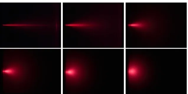
Volumetric scattering effects are important for making real-istic computer graphics images of many materials like skin, fruits, milk, clouds, and smoke. In these cases, we cannot make the common assumption that light propagates without scattering in straight lines. Indeed, the multiple scattering of light in participating media is important for many qualitative effects [Boh87a,Boh87b] like glows around light sources in foggy weather, or subsurface scattering in human skin, or the spreading of a beam in a scattering medium, as shown in Figure1.
Light transport, including multiple scattering in arbi-trary scattering media, can be accurately computed by solv-ing the radiative transfer equation [Cha60,Ish78]. Volu-metric Monte Carlo and finite element techniques (volu-metric ray tracing and radiosity) have been used by many researchers [RT87,LBC94,Max94,BSS93,PM93,JC98]. However, volumetric multiple scattering effects are notori-ously difficult to simulate. Solution times with the fastest Monte Carlo approach range anywhere from a few hours to a few days. For this reason, these effects are not usually present in computer graphics imagery. Thus, one must look for simpler approximations and models.
This paper describes a practical approach for computing lighting and volumetric effects in spatially varying inhomo-geneous scattering media, taking directionally-varying
light-ing effects into account. While simulatlight-ing multiple scatter-ing directly is computationally very expensive, the observ-able qualitative properties are simple—the incident radiance distribution is blurred and attenuated. There is spatial and an-gular spreading of incident illumination inside the material. This spreading can be expressed as a point-spread function (PSF) that formally measures the spreading of incident radi-ance in a given medium. Intuitively, the point spread func-tion tells us how the spatial and angular characteristics of light are changed due to scattering events inside the mate-rial. This enables us to formalize the light transport in vol-umes as a convolution of incident illumination and the PSF of the medium. Our approach uses the mathematical path in-tegration framework [PAS03,Tes87] to describe effects of multiple scattering in terms of spatial and angular blurring, thus avoiding costly direct numerical simulation.
The main observable consequences of multiple scattering in volumetric media are spatial and angular spreading of the incident light distribution. We characterize different types of spreading and focus on spatial spreading. We give a simple expression for the spatial spreading width of a collimated beam and compare it with Monte Carlo simulations. Once the PSF of the medium is known, we present a practical ren-dering algorithm using the PSF to compute effects of multi-ple scattering. We separate the practical rendering algorithm and its underlying principles from the mathematical details.
Figure 1:Effects of multiple scattering. Collimated light source (laser beam) is shone into a container filled with water. Milk has been added to water to add scattering particles. The photographs show effects of multiple scattering with increasing concentration of scattering particles. The effects of multiple scattering are visible as spatial and angular broadening of the laser beam.
The rendering algorithm can therefore be implemented with-out relying on heavy mathematics.
1.1. Overview
A volumetric medium acts as a point spread function that changes spatial, angular and temporal characteristics of the incident radiance (light field). What an observer sees is therefore a convolution between the incident illumination and the point spread function of the medium. The goal is to express the PSF of the medium in terms of basic optical properties (scattering coefficients and phase function) and then show how it can be efficiently used in a rendering al-gorithm. While the underlying mathematics behind detailed derivations may not be trivial, the final algorithm is quite simple:
1. Given a medium and incident illumination, find how much light is available for redistribution due to multiple scattering. This consists of computing the reduced inten-sity of light due to simple attenuation.
2. Apply the point spread function to the light volume. This is done by blurring the light volume with kernels of dif-ferent sizes and storing the light volume at various levels of detail.
3. During the rendering stage, at every point in the volume we compute how much spreading (blurring) occurs due to multiple scattering and we simply look up the result from the blurred representation of the light volume.
2. Related Work
The radiative transfer equations and their approximations have been extensively studied in many fields. We only men-tion recent practical methods in computer graphics. The in-terested reader is referred to a survey by Perez et al. [PPS97] for detailed classification of global illumination algorithms in participating media. Pharr and Hanrahan [PH00] also pro-vide an extensive list of existing methods.
One simple approximation is to only consider single scat-tering, as done by Ebert and Parent [EP90], Sakas [Sak90],
Max [Max86], Nakamae et al. [NKON90], and Nishita et al. [NDN96]. However, they cannot easily reproduce impor-tant qualitative effects due to multiple scattering like glows around light sources, or subsurface scattering.
Another approach is to use the diffusion approximation, first introduced in graphics by Stam [Sta95], following con-ceptually similar work by Kajiya and von Herzen [KH84]. More recently, Jensen et al. [JMLH01] (also Koenderink and van Doorn [KvD01]) applied it to subsurface scattering, de-riving a simple analytic formula. This provides a practical approach to a problem that had previously required an im-mense amount of computation [HK93,DEJ∗99]. However, the diffusion approximation is valid only for optically dense homogeneous media, where one can assume the angular dis-tribution of radiance is nearly uniform. It is also technically valid only for infinite plane-parallel media. Further, the ap-proach of Jensen et al. [JMLH01] is specialized to subsur-face effects on objects, and cannot be easily extended to volumes. Our method can be seen as analogous to the dif-fusion point-spread function for general media, where we handle spreading of light explicitly in arbitrary volumes. We can therefore handle spatially varying general materials, and highly directional effects.
In the context of subsurface scattering, fast integration techniques, bearing some similarity to our approach have been developed. For example, Jensen and Buhler [JB02] ex-tended the diffusion approximation to be computationally more efficient by precomputing and storing illumination in a hierarchical grid. Lensch et al. [LGB∗02] implemented this method in graphics hardware. The expensive illumination sampling is alleviated by a simple lookup in the hierarchi-cal grid. Our integration framework can be thought of as ex-tending these ideas to general spatially varying media, with strong directional effects.
Most recently, Narasimhan and Nayar [NN03] solved the spherical radiative transfer equations to derive a general for-mula for the PSF due to an isotropic point source in a spher-ical medium. Their formula applies to general homogeneous materials, and does not assume optically dense media, un-like diffusion. Their application was to the inverse prob-lem of estimating weather conditions from the glow around light sources. While the direct solution of the radiative trans-fer equations is impressive (something which our approach does not explicitly do), the result is practically limited by its restriction to homogeneous isotropic media. By contrast, our rendering algorithm allows for spatially varying partic-ipating media, and our framework accounts for anisotropic sources and visibility effects in real scenes.
The idea of using point-spread functions has been ex-plored in areas other than graphics, using statistical and other complex mathematical machinery. Stotts [Sto78] described the pulse stretching in ocean water. Given the starting point and a plane some distance away from the pulse origin, Stotts characterized stretching in terms of extra path lengths the
photons travel due to scattering. McLean et al. [MCH87] used a Monte Carlo method to track individual rays. They could compute the density of photons arriving at a fixed plane some distance away from the origin from all direc-tions and times. The results agreed well with computadirec-tions done by Stotts [Sto78]. Lutomirski et al. [LCH95] extended the statistical analysis of Stotts. They provide exact statisti-cal formulations for spatial, angular and temporal spread-ing. Additional studies of beam spreading were done by Ishimaru [Ish79] and McLean and Voss [MV91] who com-pared theoretical results with experimental measurements. Gordon [Gor94] rigorously derived equivalence of the point and beam spread functions from the radiative transfer equa-tion. McLean et al. [MFW98] described an analytical model for the beam spread function and validated their model with Monte Carlo computations. They also give a comparison with many other analytic models.
Our expression for the point spread function and the blur-ring width stems from the formulation of light transport as a sum over all paths [Tes87]. However, the derivation itself is quite different and it does not rely on heavy mathematics of path integration [APRN04].
3. Point Spread Function
A point spread function (PSF) measures the spreading of incident radiance in a given medium. Intuitively, the point spread function tells us how the spatial and angular charac-teristics of light are changed due to scattering events inside the material. For example, on a foggy day, a street light has a distinct glow around it. The diameter of the glow is deter-mined by the point spread function of the medium which in turn is a function of the optical properties of the medium. There are different types of spreading that occur as a con-sequence of the multiple scattering. We discuss these differ-ent types of spreading with focus on spatial spreading that is particularly relevant for computer graphics applications. We give a simple expression for the blurring width in the medium and compare it with a Monte Carlo experiment.
3.1. Effects of Multiple Scattering
If we shine a laser beam pulse into a scattering medium, the pulse undergoes a series of absorption and scattering events. The effects of multiple scattering result in significant changes to the pulse:
1. Spatial spreading. The pulse cross-section broadens as it propagates through media, as shown in Figure1. We in-corporate this effect into our algorithm.
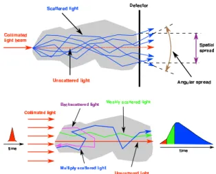
2. Angular spreading. The angular divergence of a narrow pulse gets larger as it travels through the medium. We do not currently incorporate such effects into the algorithm but provide necessary mathematical results for doing so with a procedure similar to that used for spatial blurring. 3. Temporal spreading. Scattered photons of the pulse stay behind the original unscattered photons since they have
Figure 2:Beam spreading in scattering media due to multiple scat-tering.
to take longer paths. The direct consequence is that pulse becomes longer as it travels through the medium. While this effect is very important in many fields such as re-mote sensing [WM99], it is of little interest for computer graphics which deals with stationary solutions of light transport. We will, however, see that explicit treatment of time (or distance) dependence is very useful as an in-termediate step.
Figure2illustrates spatial, angular and temporal spreading due to multiple scattering. Many of the subtle appearance effects of scattering materials are a direct consequence of beam spreading due to multiple scattering. As we see, it is straightforward to qualitatively understand beam spreading and stretching in the scattering media, but direct simulation of multiple scattering and therefore of spreading (blurring) is computationally expensive. The quantitative analysis of spatial and angular spreading we present could provide more insight into the appearance of scattering materials and could lead to more efficient and simpler rendering algorithms.
3.2. Spreading Width
The width of the beam spread in a medium depends on the amount of scattering in the medium. As shown in Figure1, the width of the beam is directly proportional to the number of scattering events in the medium. Assuming that scattering paths comprising the beam have Gaussian distribution, we derived the width of the beam spread of a collimated light beam at distance S as a function of optical properties of the medium (absorption coefficient a, scattering coefficient b, and mean square scattering anglehθ2i). We state the final result for the beam width:
w2(S) =1 2 2a 3S+ 16α bS3 −1 = hθ 2ibS3 16(1+S2/12l2), (1) with l being a diffusive path length l2=1/(abhθ2i) and α=1/(2hθ2i). A detailed derivation of the expression for
width using the path integration framework is available in a companion document [APRN04].
In a similar fashion to equation 1, one can express the angular spreading of light. In extreme cases, like the diffu-sion approximation for optically dense media, the angular distribution of light becomes nearly uniform. We currently do not explicitly consider angular blur in our approach, but an analogous expression for angular spreading is presented in [APRN04].
It is clear from equation1that the spread width is mono-tonically increasing with the distance S in the medium. The beam width also increases with the number of scattering events b. The more scattering events occur in the medium, the more the beam is spread. This can be seen in Figure1
where the width of the laser beam is much wider with in-creased concentration b of scattering particles. The beam spreading retains the directionality of the incident collimated beam until some distance s where the transition to diffusion regime occurs. At this point the light field is essentially dif-fuse and has no directionality that was present upon enter-ing the medium. This effect can also be seen in Figure1
where in the liquid with large number of scattering parti-cles (i.e. larger scattering coefficient b), light distribution quickly becomes diffuse. The beam spread width also grows faster with larger mean square scattering anglehθ2i. The more forward-peaked the phase function is, the slower the increase in the beam spread width. As expected, in the ab-sence of scattering, the beam spread width is zero and the beam is only attenuated due to absorption. The beam spread width expression also does not have an upper bound. At first glance this seems bothersome, but as we show later, the at-tenuation increases at an even faster rate.
McLean et al. [MFW98] summarize different expressions for spreading width in the medium. Our particular expres-sion in equation1has the same functional form as many other expressions with a different constant factor. Due to dif-ferent assumptions and methods, most derivations differ in the constant factor [MFW98]. Being relatively simple, our approach provides an expression for spatial blurring that is easy to evaluate. Rigorous approaches typically do not pro-vide a general closed form solution and only special cases, discussed below, can be evaluated. When we use these spe-cial cases to compare our results against these more so-phisticated theoretical methods, we find the accuracy of our method to be sufficient given the needs of computer graphics applications. This lends more solid ground to our approach.
Limiting Cases. For long paths (S l), the square
of the spatial width grows linearly with distance S along the path: w2= 34hθ2ibSl2. For another special case of no absorption (l =∞), the width is w2 =bhθ2iS3/16. For these limiting cases, using a much more rigorous deriva-tion, Tessendorf [Tes87] obtained the spatial width of w2=
bhθ2iS3/24 for case of no absorption and w2=bhθ2iSl2/2 with absorption. In comparison with Tessendorf, we obtain
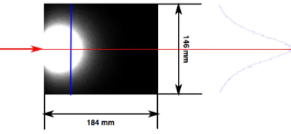
Figure 3:Monte Carlo simulation of a scattering medium. Density estimation of photons yields energy distribution in the medium. A slice through the volume taken at the laser plane (horizontal slice at the height at which photons were injected into the medium) is shown for a particular configuration. Dimensions of the simulation domain are shown as well as an actual slice through the volume. A vertical profile at some distance from the source is shown.
a correct functional dependence on both S and medium pa-rameters, but are off by a constant factor of 3/2. This dis-crepancy can be offset by multiplying our expression by a constant correction factor (in this case the correction factor is 2/3).
Absorption Effects. Note that unlike many comparable
formulations for the beam spread, our expression does have dependence on absorption in the medium. Intuitively, if ab-sorption is included, some light gets absorbed and conse-quently the spread of the beam is narrower than with scatter-ing only. This is consistent with observations that scatterscatter-ing redistributes light in all directions while absorption has just the opposite effect and tries to keep the beam collimated to minimize attenuation. For many materials of practical inter-est (e.g. clouds, water, snow), the absorption is often orders of magnitude smaller than the scattering.
3.3. Monte Carlo Comparison
To check spatial spread width predictions from the model, we compare blurring widths with Monte Carlo simulations. Scattering of a laser beam entering participating media was chosen for this testing since it provides the closest real-life analogy with the idea of a single ray. A simulation was per-formed by shooting 30 million photons into the medium and storing their energies at the position of each scattering event. Energy density estimation is done for the photons satisfying the necessary boundary conditions, in this case those with propagation direction within a small angle of the horizontal axis. A 2D slice through the simulation volume in the plane of the laser beam produces images of the type shown in Fig-ure3. A single vertical column in this image is also shown. The shape of this function can be directly compared with our expressions for spatial spreading of the beam.
Monte Carlo simulation was preferred to the real exper-imental curves because it is much easier to obtain the in-formation we need for the most direct comparison with the theory. Direct numerical comparison between actual experi-ment and Monte Carlo simulation and our model is very dif-ficult because exact optical properties for real materials are
Figure 4:Top left plot shows the average case normalized inten-sity profile compared to a Gaussian with corresponding theoretical width. Other plots show spatial spread widths for different scattering coefficients b as a function of distance along the beam. The scatter-ing medium was simulated usscatter-ing the followscatter-ing parameters: g=0.9 (hθ2i=0.24), a=0.0003mm−1.
rarely available. To validate Monte Carlo simulation results we, in turn, use them to create side views of the propagat-ing beam from outside the container and compare them with real photographs shown on Figure1. Profiles of such images were found to be very similar in shape.
Normalized cross-sections of the beam at different dis-tances from the entry point along with those predicted by the model were plotted. An example is shown in Figure4. While a significant portion of the profile is well approx-imated by a Gaussian, the figure also demonstrates that a wider non-Gaussian component not captured by our model is also present. Since this component has low magnitude compared with the main profile, we believe it will not sig-nificantly affect rendered images. A more accurate model would certainly be needed for applications where such de-tails of scattering are important. Figure4shows our average case—some curve shapes agree better with our predictions while others deviate more.
We extracted Full Width at Half Maximum (FWHM) of the beam cross-section as the function of distance from the entry point for several Monte Carlo simulations using differ-ent scattering coefficidiffer-ent b, while other values were fixed to their typical values. The results are shown in Figure4along with corresponding theoretical predictions. Noticeable blur-ring starts only after the beam travels some distance in the medium. We therefore compute blurring width by plugging in a shifted length value into our expressions which corre-sponds to a horizontal offset of calculated curves. A value of 8/b for the amount of shift gives good agreement with the experiment.
To study beam attenuation (discussed in more detail in Section4.5), we plot the dependence of light energy
den-Figure 5:Laser beam attenuation. Left: beam attenuation compar-ison between Monte Carlo simulation, Beer-Lambert exponential attenuation law, and modified exponential attenuation. Right: log-scale plot of beam attenuation.
sity along the beam axis from the distance to the beam en-try point (Figure5). We found that for the first several or-ders of magnitude, the attenuation is well described by the Beer-Lambert exponential attenuation law. The effective at-tenuation coefficient, however, is noticeably lower than our simple exp(−cs)prediction and deviation is increasing for denser media reaching about 0.45c for the densest medium we used. The attenuation coefficient given by diffusion ap-proximation does even worse job due to inapplicability of this approximation to the clearly direction-dependent case we study. Obtaining a better expression for attenuation is left as an important area of future research.
4. Mathematical Details
In this section, we introduce the mathematical preliminaries of the radiative transfer equation and path integration, nec-essary for relating the traditional light transport equation to a less commonly used convolution formulation. We provide some intuition behind the point spread function and how it relates to traditional ray tracing.
Readers more interested in implementation may wish to skip to Section5, that will use the point spread function for a practical algorithm to compute effects of multiple scatter-ing.
4.1. Radiative Transfer Equation
Optical properties of volumetric materials can be character-ized by densityρ(x), their scattering and absorption coeffi-cients b(x)and a(x), the extinction coefficient c(x) =a(x) +
b(x), and the phase function P(x,~ω,~ω0). The phase function P describes the probability of light coming from incident di-rection~ωscattering into direction~ω0at point x. The phase function is normalized,R
4πP(~ω,~ω0)dω0=1 and only de-pends on the phase angle cosθ=~ω·~ω0. The mean cosine g of the scattering angle is defined as g=R
4πP(~ω,~ω0)(~ω·~ω0)dω0 and the average square of the scattering anglehθ2iis
hθ2 i=2π Zπ 0 θ 2 P(~ω,~ω0)sinθdθ. (2) The most general case of light transport in arbitrary media is described by the time-dependent radiative transport
equa-(a) No scattering (b) Single scattering
Figure 6:Green’s propagator for the light transport equation can be related to marching along a ray and computing effects of attenu-ation operator Gnoscatterand single-scattering operator Gsingle. tion [Cha60,Ish78],
∂ ∂s+~ω· ∇+c(x) L(s,x,~ω) = b(x) Z 4π P(~ω,~ω0)L(s,x,~ω0dΩ0) +Q(s,x,~ω), (3) where we have expressed time t in units of length s, with s=vt. As compared to the standard time-independent equa-tion, we have introduced the term∂/∂s on the left-hand side. Q(s,x,~ω)is the source term, accounting for emitted illumi-nation from light sources.
From the general theory of linear integral equa-tions [BG70], it is known that the solution of equation3can be expressed as a convolution of the initial source radiance distribution Q=L0(x0,~ω0)with a Green’s function or prop-agator (evolution operator) G(s,x,x0,~ω,~ω0):
L(s,x,~ω) = Z
G(s,x,x0,~ω,~ω0)L0(x0,~ω0)dx0d~ω0. (4)
Physically, the Green propagator G(s,x,x0,~ω,~ω0) repre-sents radiance at point x in direction~ωat time s due to light emitted at time zero by a point light source located at x0 shin-ing in direction~ω0. Mathematically, it is the solution of the homogeneous version of equation 3(i.e. with source term set to zero) with initial condition expressed using the Dirac delta functionδas
G(s=0,x,~ω,x0,~ω0) =δ(x−x0)δ(~ω−~ω0). (5)
4.2. Green’s propagator and relation to raytracing
In the absence of scattering (b=0), the solution for the com-plete propagator G is almost trivial:
G(s,x,~ω,x0,~ω0)≡Gnoscatter(s,x,~ω,x0,~ω0) = δ(x−~ωs−x0)δ(~ω−~ω0)×exp − Zs 0 c(x−~ω(s−s0))ds0 . (6) Here the light travels in a straight line and is attenuated by the absorption coefficient a(x) =c(x). One can see that in this case, the formulation using the propagator is equiva-lent to simple raytracing (Figure6). This simple attenuation model is quite popular in computer graphics and it is often part of popular APIs like OpenGL (fog attenuation).
We can also write the propagator G to include an arbi-trary number of scattering events. For example, single scat-tering propagator Gsingleincludes light that has been scat-tered only once and the light that has not been scatscat-tered at all (as above). To formalize it, we note that propagation from starting position and direction(x0,~ω0)to final position and direction(x,~ω)requires three steps. First, light is attenuated over distance s0to an intermediate point x00. Second, the light scatters at point x00from initial direction~ω0to final direction ~ω. Only a fraction that is determined by the phase function P of the incident radiance scatters into the new direction. Third, light is further attenuated from the intermediate point
x00to the final point x0. To include all possible intermediate points where a scattering event occurs, the propagator Gsingle is given by integration over all intermediate points:
Gsingle(s,x,~ω,x0,~ω0) =Gnoscatter(s,x,~ω,x0,~ω0) + Zs 0 ds0 Z |x00−x0|=s0 Z S2 Gnoscatter(s−s 0,x,~ω,x00,~ω000)×b(x00)(7) Z S2P(x 00,~ω00,~ω000)Gnoscatter(s0,x00,~ω00,x0,~ω0)dω00dω000dx00. This expression again directly corresponds to the standard single scattering ray marching algorithm commonly used in computer graphics. Marching along the viewing ray and sending shadow rays (that are also attenuated) toward a light source corresponds to the three steps discussed above (Fig-ure6).
We could further rewrite the propagator to include higher order of scattering events by recursively expanding the prop-agator. But, as demonstrated by equation7, the expression would quickly become unmanageably complex due to addi-tional angular integrations that have to be performed to ac-count for higher orders of scattering. Therefore, it is often useful in practice to split the propagator G into two parts: un-scattered and single-un-scattered (or “direct”) light Gd=Gsingle and one for multiply scattered (or “indirect”) light Gsand solve them separately:
G(s,x,~ω,x0,~ω0) =Gd(s,x,~ω,x0,~ω0) +Gs(s,x,~ω,x0,~ω0) (8) The initial condition for the scattered light propagator Gsis straightforward, because there is no multiply scattered light in the beginning:
Gs(s=0,x,~ω,x0,~ω0) =0 (9) We will use existing techniques for computing direct lighting described by Gd. Our main goal in this work will be to efficiently deal with propagator Gs(multiply-scattered light) that could lead to faster rendering algorithms for par-ticipating media.
4.3. Path Integral Formulation
The path integral (PI) approach provides a particular way to express the propagator G(s,x,~ω,x0,~ω0). It is based on the simple observation that the full process of energy transfer from one point to another can be thought of as a sum over
transfer events taking place along many different paths con-necting points x and x0, each subject to boundary conditions restricting path directions at these points to~ω and~ω0, re-spectively. The full propagator is then just an integral of in-dividual path contributions over all such paths. This object is called the path integral. One can further notice that the in-tensity of light traveling along each path will be only dimin-ishing due to absorption and scattering events along the path. This is because in-scattering into the path, which is generally treated as a process increasing light intensity, in a particular direction will be due to photons traveling a different path in the medium (we ignore here exact backscattering which can return photons exactly to the same path). Therefore, if we introduce effective attenuationτalong the path, we can write the individual path contribution (weight) as exp(−τ), and the complete propagator as
G∼
Z
exp(−τ(path))Dx, (10) where the attenuationτis analogous to the classical action A along the path, with exp(−τ(path))∼exp(−A(path)).
Because the integration is performed over the infinite-dimensional path space using highly non-intuitive differ-ential measure Dx defined for it, the mathematics of path integrals is exceptionally complex [FH65,LRT82]. Tessendorf [Tes89] derived a path integral expression for the propagator G in homogeneous materials. Interested read-ers are referred to his further work [Tes91,Tes92] for de-tailed derivations of the path integral formulation. Using much simpler tools, one can still obtain some useful re-sults [PAS03] of the PI theory, which we will present here without detailed derivations.
First, part of path weight or action due to multiple scatter-ing in the integral in equation10can be shown to be propor-tional to:
exp(−A(path))∼
exp − Z s 0 " a(~γP(s0)) + α b(~γP(s0)) dθ ds0 2# ds0 ! , (11) where~γ(s)is a path length parameterized path, dθ/ds is its curvature, andα=1/4(1−g) =1/(2hθ2i), wherehθ2iis the mean square scattering angle. Integration is performed along the path.
One can find a path which maximizes this expression (i.e. has minimal attenuation or action among all possible paths). We call it the most probable path (MPP). For the important special case of homogeneous media under boundary condi-tions when path direccondi-tions are specified at both ends, one can determine the shape of MPP of given length analyti-cally with the standard Euler-Lagrange minimization proce-dure [Fox87]. The result is a “uniformly turning” path of constant curvature which is changing its direction at a con-stant rate.
We further assume that only a small fraction of paths
Figure 7: Once we find a set of most probable paths for given initial conditions, we compute contributions along those paths and some neighborhood around these paths. All other paths are ignored because they are deemed not important. In practice, we do not even consider the full set of MPPs, but rather a subset of those which are the easiest to treat.
“around” the MPP contribute significantly to the integral and will restrict the integral to account for the contribu-tion of these important paths only. Formally, this constitutes a Wentzel-Kramer-Brillouin (WKB) expansion [LRT82] of the path integral while physically and visually it accounts for the fact that blurring of the radiance distribution is the most notable characteristic of participating media. The basic idea of our approach, using the most probable path, and a neighborhood around it, is shown in Figure7.
4.4. Surrounding Path Contribution
In computer graphics, a boundary condition of particular in-terest is a single-sided one, which requires the path to start at a particular point in space with particular initial direction (an example is the eye position and primary viewing ray direc-tion) but applies no additional restrictions on the second end of the path. The path will usually terminate once it reaches an object (or a light source) in the scene. Suppose we found the MPP for this boundary condition and computed its con-tribution. We would now like to approximate the complete path integral by taking into account only the contribution of “surrounding” paths. This operation formally constitutes a WKB expansion of the integral.
If we parameterize the family of nearby paths using some vector of parameters~ξ(with~ξ=0 at the MPP), the path in-tegral can be written as an inin-tegral over these parameters. Note that because A in equation11has the global minimum at the MPP, its expansion in terms of parameters~ξwill start from square terms. That is, if there is only one parameterξ, a simple Taylor series is,
A(ξ) = A(0) +1 2ξ
2∂2A ∂ξ2 +. . ., exp(−A(path)) ∼ exp(−A(MPP))exp −1
2ξ 2∂2A ∂ξ2 ! , (12) where the linear term in the top equation is omitted because A(0)is a minimum, and A(0)corresponds to the action for the most probable path. Note that the bottom equation has a Gaussian form, giving weights to nearby paths according to
their “distance” from the MPP. If~ξis now a vector, we may write the propagator in equation10as
G∼exp(−A(MPP)) Z
ξexp(−(ξ∇ξ)
2
A/2)dξ. (13) The first term here is the MPP contribution and the integral is over re-parameterized path space. Although integration space is still infinite-dimensional, we can use this expression to estimate some important properties of the radiance distri-bution by writing out the expansion of A for some family of nearby paths in terms of relevant parameters while keeping others fixed. In particular, we will be interested in radiation blurring along the path, which can be measured by the spa-tial width of contributing paths.
4.5. Full Propagator
So far we considered different parts of multiply-scattered light propagator Gs as suited our needs. We now put ev-erything together and write the full approximate expression which will be directly used by the rendering algorithm. To obtain full energy transfer expression, we multiply the con-tribution of each path by its probability and sum over all paths. Note that from statistical point of view, this is just the expected value of “standard” single path attenuation exp(−Rs
0c(~γ(s0))ds0)over the pdf of paths given by equa-tion11. We can therefore write Gsas
Gs(s,x,~ω,x0,~ω0) = Z exp − Zs 0 c(~γ(s0))ds0 Cexp(−A(~γ(s0)))Dx (14) The first factor simply states that light which scatters out of the path (or absorbed along it) is lost as far as the given path is concerned and is analogous to Gnoscatter present in the expression for Gsingle, equation7. The second factor is due to accounting for probability of the specific sequence of scattering events (and absence of any absorption ones) which forced this particular path and not any other to be chosen and C is a normalization constant.
An expression for multiply scattered radiance is obtained using general equation4. Singly scattered (per unit length) radiance bL0 serves as the source Q for multiply scattered light, leading to Ls(s,x,~ω) = Z x0,~ω0 Z exp − Zs 0 c(~γ(s0))ds0 Cexp(−A(~γ(s0)))Dxb(x0)L0(x0,~ω0)dx0d~ω0 (15) We will now replace integral over complete path space with that over only paths surrounding the MPP, treating the first term in equation14as approximately the same for all such paths and take it out of the path integral. The second term can be expressed by equation12and exp(−A(MPP)) is also taken out of the path integral. The rest of the path integral gives simply the fraction of all paths which satisfy boundary conditions regardless of the specific path shape
(but adjusted for absorption to avoid double-counting since this is already included in the first term in equation14). For simplicity, we consider here only directional light sources and assume that single scattered light distribution is strongly forward peaked, ignoring angular spreading introduced by single scattering event. This means that path fraction is di-rectly given by the multiply-scattered phase function PMS which gives the probability of light being scattered by a given angle after given number of scattering events. Only the integration over the support of the Gaussian remains:
L(s,x,~ω) =exp − Z s 0 c(MPPs(s0))ds0 exp(−Ac(MPPs)) ×PMS(~ω−~ω0) Z plane⊥MPPgauss(x 0,w(s))b(x0)L0(x0,~ω0)dx(16)0
where gauss(x0,w(s))is a Gaussian of width w(s)given by expression1applied at position x0and Acrepresents the cur-vature part of the action function. Parameter s emphasizes that MPPsis constructed for given total length s. Explicit in-tegration over complete(x0,~ω0)-space present in the original expression is replaced by integration over its much reduced subset selected by the set of MPPs we consider. This is the key to efficiency of algorithms based on WKB expansion of the path integral. For arbitrary light sources, directional integration will remain and can be performed using similar procedures and expressions for angular blurring [APRN04].
INHOMOGENEOUS MEDIA. The final step is to recall
that in computer graphics we need a time-independent so-lution given by integration of expression 16 over all path lengths s. We also note that since only integrals along paths are used, the result does not depend on whether the medium is homogeneous or not (but, in general, the set of MPPs will). It is useful therefore to write final expressions using the total number of scattering events along the path`=R
b(~γ(s0))ds0: L(x,~ω) = Z `d`exp(−(c/b)`(MPP`))exp(−Ac(MPP`)) ×PMS(`,~ω−~ω0)Z plane⊥MPP gauss(x0,w(`))L0(x0,~ω0)dx0, (17) Multiply-scattered phase function in WKB approximation is given by Tessendorf and Wasson [TW94] as PMS(`,θ,) = (1/N)P(θ/p
`/(1−exp(−`))) with new normalization constant N introduced to ensure thatR
PMS(`,θ)dω=1. We can also re-parameterize our (2/3)-corrected expression1for blurring width as
w2= hθ
2i` S2
24(1+hθ2i(a/b)`2/12). (18) As will be clear from our algorithm, we will be avoiding con-structing curved MPPs which was shown to be quite compli-cated [PAS03]. Under such conditions, keeping the curva-ture term in Ac(MPP)in its exact form is an overkill and we can simplify it toR α β dθ ds0 2 ds0≈α(∆θ)2/`where∆θis the total angle change along the path. This completes the deriva-tion. In section5we will describe the procedure we use to efficiently implement calculation suggested by equation17.
Algorithm 1Preprocessing
function PreprocessVolume(Volume V) for each light source Si
Li= ComputeLightAttenuationVolume( V , Si) BuildVolumePyramid( Li)
function ComputeLightAttenuationVolume(Volume V, Light S) for each voxel xiin V
// Compute transmittance T from voxel xito // light source S (xlight) – see Figure8. T = exp( - c * Distance(xi, xlight)) Store Li= T * LightIntensity( S ) in voxel xi function BuildVolumePyramid(Light Volume LV) for each level l (from 1 to log2(size)) in LV
Resample level l−1 to half the size
Apply Gaussian filter with widthσto downsampled volume
5. Rendering Algorithm
Our implementation sacrifices the accuracy of computation for efficiency by making a number of further simplifications to deal with already simplified but still rather complex equa-tion16. We believe that since the main observable conse-quence of multiple scattering is blurring, it is not crucial to accurately reproduce the result of such a process as long as its most general characteristics (for example, the degree of blurring with the distance to the observer) are captured. A process which results in loss of detail should not incur a dra-matic computational penalty as is the case with most existing rendering algorithms. The pseudocode for the rendering al-gorithm is summarized in Alal-gorithm 2.
As aPRECOMPUTATION STEP, we first compute the at-tenuated light volume for every light source (function Com-puteLightAttenuation in Algorithm 1). From every voxel xi in the volume, we send rays towards a light source (xlight), compute attenuation along the ray and store the intensity in the voxel. We currently compute a separate light volume for each light source. The purpose of this precomputation is to build an efficient data structure such that we can quickly lookup how much light is available for redistribution at any point in the volume. We also build a hierarchical represen-tation of this data structure (function BuildVolumePyramid in Algorithm 1). This hierarchy allows us to get lighting in-formation at different scales. It is built by applying a set of Gaussian filters with different standard deviationsσto the attenuated light volume. The standard deviationσ can be chosen based on the optical properties of the medium to bet-ter cover the expected range of blurring widths w (from 0 to a user specified maximum width). The filter width for every level is stored with the rest of the data. We use iterative filter-ing to accelerate the construction process. The blurred light can be stored at full resolution but it is wasteful to do so, be-cause detail is removed by Gaussian blurring. After blurring we also resample the volume with a tent filter to produce a lower level stored in a pyramid. Therefore, the hierarchy
Figure 8:To speed up multiple scattering computation we approx-imate a true curved path with two line segments and compute the blur width that occurred along this path. We then spatially blur the incident radiance and apply proper attenuation to compute the con-tribution of paths within this cone to multiple scattering.
is essentially a three-dimensional mip-map. There are var-ius data structures that can holding blurred lighting infor-mation. Our particular implementation is a variation of the deep shadow map [LV00]. For a reasonably sized volumes (1283voxels), creation of the light pyramid takes under 10 seconds.
DURING RENDERING, we sum up contributions along light paths. Although the true light path is curved, we instead approximate true path with two linear segments as shown on Figure8. We refer to computation steps in Algorithm 2. We start by stepping into the media along the viewing ray by some distance s1(line 1) to arrive at point x1. We then con-struct a line segment from x1to the exit point xlightin the di-rection of a light source. This segment has length s2(line 2) and its corresponding number of scattering events is`2(line 6). We then get the radiance at point x1 from our blurred light volume data structure. The level of the pyramid is cho-sen based on the blurring width given by equation1(line 8) for the total approximate length of the path S=s1+s2. At each level we have stored the blur width that we used during precomputation. We search through the widths in the light volume pyramid to find the corresponding level. If necessary, we interpolate between two different levels like in standard texture mip-mapping (line 9). The multiple scattering contri-bution has effectively been reduced to a simple table lookup. Thus far we have determined spatial spreading due to multi-ple scattering, but have not yet accounted for attenuation. We multiply spatially spread radiance by the necessary attenua-tion given by remaining terms in equaattenua-tion16: phase function (line 11), path curvature (line 12), and attenuation (line 13). To find the next sampling point, we project the blur width onto the viewing ray along the light direction to determine the next sampling point as shown on Figure9. This avoids counting the same light contribution more than once. Some moderate overlap still occurs but it can be controlled by in-creasing step size if it presents a problem. The side effect of this process is that the step size gets progressively larger as
Figure 9: To choose the next sampling point (red circle), we project a sphere with radius equal to the blur width along the line onto the viewing ray. This process is repeated until the ray exits the volume or entire ray has been covered by contributions due to mul-tiple scattering.
Algorithm 2Rendering algorithm summary
function L = MultipleScattering( Light Volume LV ) //α=1/4(1−g)
// PMS(theta, `) =N∗P(theta/ p
`/(1−exp(−`)))
// N - precomputed PMSnormalization for each sampling point xi
(1) s1=Distance(xi,xcamera) (2) s2=Distance(xi,xlight) (3) S=s1+s2
(4) d`=Distance(xi,xi−1)∗b
(5) Compute scattering number`1=`1+d`
//`2can be precomputed in ComputeLightAttenuationVolume (6) Compute scattering number`2
(7)`=`1+`2
(8) Compute blur width w= r
hθ2i`S2
24(1+hθ2i(a/b)`2/12)
// Lookup() returns precomputed attenuated radiance L // from the mip-map at point xiand blurring level w // Multiple scattering contribution has
// been reduced to a simple lookup in the table (9) L = Lookup(xi, LV, w)
(10) theta = arccos(~ω·~ω0)// scattering angle
(11) P = PMS(theta, `)// Multiple scattering phase function (12) C =α∗theta2/`// Path curvature
// Weight multiple scattering contribution (13) weight = exp( -(c/b)`) * exp( -C ) * P // Add multiple scattering contribution (15) Ltotal = Ltotal + L*weight return Ltotal
we march along the ray since the blur width is monotonically increasing with the distance.
For inhomogeneous media, the computational procedure is similar. The only difference is that due to spatial variation of optical properties, we need to integrate scattering coeffi-cient along the path:`=R
b(xstart+s0~ω)ds0. Since`along the path is expensive to compute during rendering, we com-pute and store`2(light part of the path) in another data struc-ture during preprocessing. This does not lead to any increase
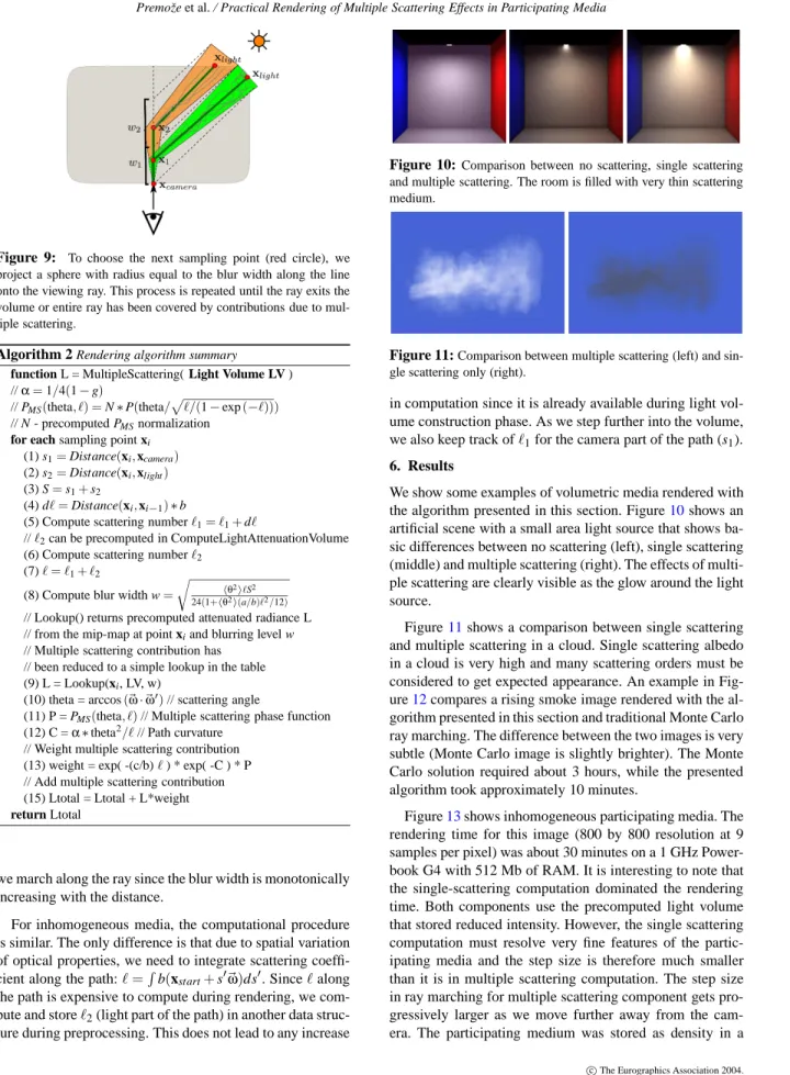
Figure 10:Comparison between no scattering, single scattering and multiple scattering. The room is filled with very thin scattering medium.
Figure 11:Comparison between multiple scattering (left) and sin-gle scattering only (right).
in computation since it is already available during light vol-ume construction phase. As we step further into the volvol-ume, we also keep track of`1for the camera part of the path (s1).
6. Results
We show some examples of volumetric media rendered with the algorithm presented in this section. Figure10shows an artificial scene with a small area light source that shows ba-sic differences between no scattering (left), single scattering (middle) and multiple scattering (right). The effects of multi-ple scattering are clearly visible as the glow around the light source.
Figure11shows a comparison between single scattering and multiple scattering in a cloud. Single scattering albedo in a cloud is very high and many scattering orders must be considered to get expected appearance. An example in Fig-ure12compares a rising smoke image rendered with the al-gorithm presented in this section and traditional Monte Carlo ray marching. The difference between the two images is very subtle (Monte Carlo image is slightly brighter). The Monte Carlo solution required about 3 hours, while the presented algorithm took approximately 10 minutes.
Figure13shows inhomogeneous participating media. The rendering time for this image (800 by 800 resolution at 9 samples per pixel) was about 30 minutes on a 1 GHz Power-book G4 with 512 Mb of RAM. It is interesting to note that the single-scattering computation dominated the rendering time. Both components use the precomputed light volume that stored reduced intensity. However, the single scattering computation must resolve very fine features of the partic-ipating media and the step size is therefore much smaller than it is in multiple scattering computation. The step size in ray marching for multiple scattering component gets pro-gressively larger as we move further away from the cam-era. The participating medium was stored as density in a
Figure 12: Rising smoke column rendered with our algorithm (left) and reference image rendered with Monte Carlo raytracing (right).
Figure 13:Cornell box with inhomogeneous participating media. Effects of multiple scattering are clearly visible as the glow around the light source that cannot be captured by single scattering compu-tation only.
volume grid containing 1283 voxels. The scattering coef-ficients are then computed from density by multiplying it by scattering cross-sections of the volume: a(x) =Cabsρ(x) and b(x) =Cscaρ(x), where Cabs is the absorption cross-scattering, Cscais the scattering cross-section, andρ(x)is the density of the medium at point x. This requires 8 Mb of stor-age. The light volume pyramid required 32 Mb, and the pre-computed value of`2required an additional 8 Mb. While the storage requirements are moderate, they are not insignificant for large volumes. Monte Carlo methods with standard vari-ance reduction techniques (e.g. importvari-ance sampling, Rus-sian roulette, etc.) took almost 12 hours to compute, but it required less memory (8 Mb). Figure14shows multiple scat-tering in homogeneous participating medium illuminated by a spotlight.
Figure 14: Multiple scattering in homogeneous participating medium.
7. Discussion and Future Work
We have presented a practical technique for rendering effects of multiple scattering in volumetric media. We avoid direct numerical simulation of multiple scattering by taking advan-tage of spatial spreading. At the heart of our method is the expression for blurring width and the point spread function derived from a path integral analysis of light transport. While the PSF is derived under simple assumptions, effectively cal-culating the path width for spreading of a beam in a homo-geneous medium, it can be applied to inhomohomo-geneous media as well. The expression is reasonably accurate, as shown by comparison to both previous theoretical results, and Monte Carlo simulations. Since we are primarly interested in qual-itative effects of multiple scattering and not numerical accu-racy, this approximation is reasonable in practice. The main benefit is that the qualitative features of multiple scattering, such as spatial blurring of incident radiance, are computed more efficiently than previous methods. While the mathe-matics of the derivation are somewhat involved, the practical implementation is relatively simple. Further computational savings are obtained by using a progressively larger step size in ray marching since the blur size monotonically in-creases with distance. The net result is a practical algorithm that captures the characteristic effects of multiple scattering in a fraction of the time required by Monte Carlo simulation methods.
There are disadvantages to our approach, that form in-teresting directions of future work. From a theoretical per-spective, we consider only the overall statistics of the phase function, not its particular shape. This and other approxima-tions result in some quantitative differences with respect to Monte Carlo simulations. Furthermore, the computation of multiply scattered light attenuation in our algorithm is not straightforward, and is worth investigating further. From a
practical perspective, the main disadvantage of the current implementation is that we precompute the light attenuation volume for each light source. While this is simply an opti-mization or time-space tradeoff, it can become quite expen-sive for a large number of light sources. We would benefit from a more efficient data structure for the lighting volume, that stored the incident lighting distribution at each point in a compact representation like spherical harmonics.
In summary, multiple scattering effects like spatial blur-ring give rise to some of the most distinctive features in vol-umes and participating media. Previous approaches have in-volved very expensive Monte Carlo simulations. We have shown that the same qualitative effects can be obtained in a ray marching algorithm using a point spread function that blurs incident illumination.
Acknowledgements
We would like to thank Jerry Tessendorf for helpful discus-sions of the path integral formulation. This work was sup-ported in part by grants from the National Science Founda-tion (CCF #0305322 on Real-Time VisualizaFounda-tion and Ren-dering of Complex Scenes) and Intel Corporation (Real-Time Interaction and Rendering with Complex Illumination and Materials).
References
[APRN04] ASHIKHMINM., PREMOŽES., RAMAMOORTHIR., NAYARS.: Blurring of Light due to Multiple Scattering by the Medium: a Path Integral Approach. Technical report CUCS-017-04, Columbia University, April 2004.3,4,8 [BG70] BELLG. I., GLASSTONES.: Nuclear Reactor Theory. Van Nostrand
Rein-hold, New York, 1970.6
[Boh87a] BOHRENC. F.: Clouds in a glass of beer. John Wiley and Sons, 1987.1 [Boh87b] BOHRENC. F.: Multiple scattering of light and some of its observable
con-sequences. American Journal of Physics 55, 6 (June 1987), 524–533.1 [BSS93] BLASIP., SAECB. L., SCHLICKC.: A rendering algorithm for discrete
volume density objects. Computer Graphics Forum 12, 3 (1993), 201–210. 1
[Cha60] CHANDRASEKARS.: Radiative Transfer. Dover, New York, 1960. 1,6 [DEJ∗99] DORSEYJ., EDELMANA., JENSENH., LEGAKISJ., PEDERSENH.:
Mod-eling and rendering of weathered stone. In Proceedings of SIGGRAPH (1999), pp. 225–234.2
[EP90] EBERTD., PARENTR.: Rendering and animation of gaseous phenomena by combining fast volume and scanline a-buffer techniques. In Proceedings of SIGGRAPH (1990), pp. 357–366.2
[FH65] FEYNMANR. P., HIBBSA. R.: Quantum mechanics and path integrals. McGraw-Hill Higher Education, 1965.7
[Fox87] FOXC.: An Introduction to the Calculus of Variations. Dover, New York, 1987.7
[Gor94] GORDONH. R.: Equivalence of the point and beam spread functions of scatterin g media: A formal demonstration. Applied Optics 33, 6 (February 1994), 1120–1122.3
[HK93] HANRAHANP., KRUEGERW.: Reflection from layered surfaces due to sub-surface scattering. In Proceedings of SIGGRAPH (August 1993), pp. 165– 174.2
[Ish78] ISHIMARUA.: Wave Propagation and Scattering in Random Media. Volume 1: Single Scattering and Transport Theory. Academic Press, 1978.1,6 [Ish79] ISHIMARUA.: Pulse propagation, scattering, and diffusion in scatterers and
turbulence. Radio Science 14 (1979), 269–276.3
[JB02] JENSENH. W., BUHLERJ.: A rapid hierarchical rendering technique for translucent materials. ACM Transactions on Graphics 21, 3 (July 2002), 576– 581.2
[JC98] JENSENH. W., CHRISTENSENP. H.: Efficient simulation of light transport in scenes with participating media using photon maps. In Proceedings of SIGGRAPH (July 1998), pp. 311–320.1
[JMLH01] JENSENH., MARSCHNERS., LEVOYM., HANRAHANP.: A practical model for subsurface light transport. In Proceedings of SIGGRAPH (2001), pp. 511–518. 2
[KH84] KAJIYAJ., HERZENB.: Ray tracing volume densities. In Proceedings of SIGGRAPH (1984), pp. 165–174.2
[KvD01] KOENDERINKJ. J.,VANDOORNA. J.: Shading in the case of translucent objects. In Proc. SPIE Vol. 4299 Human Vision and Electronic Imaging VI (2001), Rogowitz B. E., Pappas T. N., (Eds.), pp. 312–320. 2
[LBC94] LANGUENOUE., BOUATOUCHK., CHELLEM.: Global illumination in presence of participation media with general properties. In Proceedings of Eurographics Rendering Workshop (1994), pp. 69–85.1
[LCH95] LUTOMIRSKIR. F., CIERVOA. P., HALLG. J.: Moments of multiple scat-tering. Applied Optics 34, 30 (October 1995), 7125–7136.3
[LGB∗02] LENSCHH. P. A., GOESELEM., BEKAERTP., KAUTZJ., MAGNORM. A., LANGJ., SEIDELH. P.: Interactive rendering of translucent objects. In Proceedings of Pacific Graphics (2002).2
[LRT82] LANGOUCHEF., ROEKAERTSD., TIRAPEGUIE.: Functional Integration and Semiclassical Expansions. D. Reidel Publishing Company, 1982.7 [LV00] LOKOVICT., VEACHE.: Deep shadow maps. In Proceedings of ACM
SIG-GRAPH (July 2000), pp. 385–392.9
[Max86] MAXN.: Atmospheric illumination and shadows. In Proceedings of SIG-GRAPH (1986), pp. 117–124.2
[Max94] MAXN.: Efficient light propagation for multiple anisotropic volume scat-tering. In Proceedings of Eurographics Rendering Workshop (1994), pp. 87– 104.1
[MCH87] MCLEANJ. W., CRAWFORDD. R., HINDMANC. L.: Limits of small angle scattering theory. Applied Optics 26 (1987), 2053–2054. 3
[MFW98] MCLEANJ. W., FREEMANJ. D., WALKERR. E.: Beam spread function with time dispersion. Applied Optics-LP 37, 21 (July 1998), 4701–4711. 3, 4
[MV91] MCLEANJ. W., VOSSK. J.: Point spread function in ocean water: Com-parison between theory and experiment. Applied Optics 30, 15 (May 1991), 2027–2030.3
[NDN96] NISHITAT., DOBASHIY., NAKAMAEE.: Display of clouds taking into account multiple anisotropic scattering and sky light. In Proceedings of SIG-GRAPH (1996), pp. 379–386.2
[NKON90] NAKAMAEE., KANEDAK., OKAMOTOT., NISHITAT.: A lighting model aiming at drive simulators. In Proceedings of SIGGRAPH (1990), pp. 395– 404.2
[NN03] NARASIMHANS., NAYARS.: Shedding light on the weather. In Computer Vision and Pattern Recognition (2003). 2
[PAS03] PREMOŽES., ASHIKHMINM., SHIRLEYP.: Path integration for light trans-port in volumetric materials. In Proceedings of the Eurographics Symposium on Rendering (2003). 1,7,8
[PH00] PHARRM., HANRAHANP.: Monte Carlo evaluation of non-linear scattering equations for subsurface reflection. In Proceedings of SIGGRAPH (2000), pp. 75–84. 2
[PM93] PATTANAIKS., MUDURS.: Computation of global illumination in a par-ticipating medium by Monte Carlo simulation. Journal of Visualization and Computer Animation 4, 3 (1993), 133–152.1
[PPS97] PEREZF., PUEYOZ., SILLIONF.: Global illumination techniques for the simulation of participating media. In Proceedings of Eurographics Rendering Workshop (1997), pp. 309–320. 2
[RT87] RUSHMEIERH., TORRANCEK.: The zonal method for calculating light intensities in the presence of a participating medium. In Proceedings of SIG-GRAPH (1987), pp. 293–302.1
[Sak90] SAKASG.: Fast rendering of arbitrary distributed volume densities. In Euro-graphics 90 (1990), pp. 519–530. 2
[Sta95] STAMJ.: Multiple scattering as a diffusion process. In Proceedings of Euro-graphics Rendering Workshop (1995), pp. 41–50.2
[Sto78] STOTTSL. B.: Closed form expression for optical pulse broadening in mul-tiple -scattering media. Applied Optics 17 (1978), 504–505. 2,3 [Tes87] TESSENDORFJ.: Radiative transfer as a sum over paths. Phys. Rev. A 35
(1987), 872–878. 1,3,4
[Tes89] TESSENDORFJ.: Time-dependent radiative transfer and pulse evolution. J. Opt. Soc. Am. A, 6 (1989), 280–297.7
[Tes91] TESSENDORFJ.: The Underwater Solar Light Field: Analytical Model from a WKB Evaluation. In SPIE Underwater Imaging, Photography, and Visibility (1991), Spinrad R. W., (Ed.), vol. 1537, pp. 10–20. 7
[Tes92] TESSENDORFJ.: Measures of temporal pulse stretching. In SPIE Ocean Optics XI (1992), Gilbert G. D., (Ed.), vol. 1750, pp. 407–418.7 [TW94] TESSENDORFJ., WASSOND.: Impact of multiple scattering on simulated
infrared cloud scene images. In Proceedings SPIE. Characterization and propagation of sources and backgrounds (1994), vol. 2223, pp. 462–473. 8 [WM99] WALKERR. E., MCLEANJ. W.: Lidar equations for turbid media with pulse

![Discours de M. Gaston E. Thorn, President de la Commission des Communautes europeennes. Troisieme conference des Ministres europeens responsables de affaires culturelles, Luxembourg, 5-7 mai 1981 = Speech [on cultural affairs] by Gaston Thorn, President o](data:image/gif;base64,R0lGODlhAQABAIAAAP///wAAACH5BAEAAAAALAAAAAABAAEAAAICRAEAOw==)