Asymptotic Behavior of Heterogeneous TCP Flows
and RED Gateway
Peerapol Tinnakornsrisuphap
, Member, IEEE,
and Richard J. La
, Member, IEEE
Abstract—We introduce a stochastic model of a bottleneck ECN/RED gateway under a large number of heterogeneous TCP flows, i.e., flows with diverse round-trip delays and session dynamics. We investigate the asymptotic behavior of the system and show that as the number of flows becomes large, the buffer dynamics and aggregate traffic simplify and can be accurately described by simple stochastic recursions independent of the number of flows, resulting in a scalable model. Based on the Central Limit analysis in the paper, we identify the sources of fluctuations in queue size and describe the relationship between the system parameters such as the marking function and variance of queue size. A closed-form approximation for the mean queue size as a function of system parameters is provided from a simple steady-state analysis. Numerical examples are provided to validate our results.
Index Terms—Congestion control, modeling, stochastic systems.
I. INTRODUCTION
W
ITH THE GROWING size and popularity of the Internet as a medium for exchanging information and conducting business, there has been growing interest in modeling and under-standing Internet traffic. Accurate modeling of Internet traffic is also important from the perspective of deploying differenti-ated services since it is likely that best-effort traffic will com-prise a significant portion of the Internet traffic in the foresee-able future.Today’s Internet traffic consists of many heterogeneous traffic sources, the majority of which utilize the Transmission Control Protocol (TCP) congestion control mechanism [8]. Some applications, such as File Transfer Protocol (FTP), are relatively long-lived, while others are typically short-lived, e.g., Web browsing. Characterizing and modeling TCP traffic yield an understanding of the interactions between the transport layer (TCP) and the network layer.
To this end, researchers have proposed a number of dif-ferent models, from detailed single flow models to predict the throughput of a single flow as a function of round-trip delay and packet loss probability [1], [10], [12] to linearized and nonlinear fluid models motivated by a control theoretic view-point [6], [15]. As a result, the behavior of a single long-lived TCP flow is relatively well understood. However, despite these
Manuscript received September 13, 2004; approved by IEEE/ACM TRANSACTIONS ONNETWORKINGEditor S. Low.
P. Tinnakornsrisuphap is with the Systems Engineering Group, Corporate Re-search and Development, Qualcomm, Inc., San Diego, CA 92121 USA (e-mail: [email protected]).
R. J. La is with the Department of Electrical and Computer Engi-neering, University of Maryland, College Park, MD 20742 USA (e-mail: [email protected]).
Digital Object Identifier 10.1109/TNET.2005.863453
efforts, there remain several aspects of TCP that are not well understood, especially in the context of designing good active queue management (AQM) mechanisms that will interact with many TCP flows.
The introduction of AQM mechanisms adds additional com-plexity to accurate modeling of the interaction of TCP flows with the network layer. The problem is further compounded by the heterogeneous round-trip delays of flows. In addition, much of modeling emphasis in the past was placed on understanding the behavior of long-lived TCP flows [12] and the role of session dynamics (connection arrivals and departures) has been largely ignored in modeling the interaction of TCP flows with the net-work layer, i.e., drop-tail gateways and AQM mechanisms.
Accurate modeling of individual TCP flows requires modeling of complex dynamics rising from the additive-in-crease/multiplicative-decrease (AIMD) mechanism of TCP protocol, session dynamics, and heterogeneous round-trip delays in conjunction with the underlying network layer. As the size of state space explodes with the number of sessions, this represents a major obstacle to modeling the interaction of many TCP flows in a realistic setting. For the same reason, even numerical experiments become computationally prohibitive, and fail to provide an insight into the complex dynamics.
The existing literature on TCP traffic modeling usually skirts these major obstacles by relying on ad hoc assumptions, which causes the model to be accurate only in certain regimes. Hollot et al.model short-lived TCP flows as exponential pulses, i.e., time-shifted, increasing exponential functions of limited dura-tions, whose interarrival times are exponentially distributed, i.e., Poisson process [7]. The statistics of these exponential pulses can be characterized through a time-reversal of a well-known class of processes calledshot-noise processes. This model as-sumes that the short-lived flows last only a few round-trip times and do not experience packet drops or marks, thereby implicitly assuming that congestion level is relatively low. Furthermore, flows are always in either congestion avoidance (long-lived con-nections) or slow start (short-lived concon-nections), and do not tran-sition from one to the other. In other words, the session dy-namics, where connections arrive and leave the network after transfers are completed, are not explicitly modeled. A similar approach to modeling short-lived flows is also taken in [11].
At the other end of the spectrum, Kherani and Kumar [9] suggest that as the capacity of a bottleneck link serving TCP flows withhomogeneousround-trip times (RTTs) becomes very small, this queue can be accurately described as a processor sharing queue. When the capacity is large, however, this pro-cessor sharing model becomes less accurate as newly arrived TCP flows cannot fully utilize their allocated bandwidth. In fact,
in the large capacity regime these short-lived flows may termi-nate even before they can increase their transmission rates to fully utilize their share of bandwidth.
The shortcomings of these models suggest a need for aunified model that is accurate inallregimes, instead of being restricted to a specific regime. Recently, there has been an increasing in-terest inmacroscalemodeling of TCP flows [2], [16], [20]. Un-like in microscale models where each individual TCP flow is modeled in detail, macroscale models can be developed by sys-tematically applying limit theorems to derive limiting traffic models. Since the number of connections that share a bottle-neck link inside a network is likely to be large, especially in the core network or on a transcontinental link, such a macroscale model promises a potential to provide an accurate and yet scal-able model without having to introduce any ad hoc assumptions. In this paper, we present a stochastic model of a RED gateway [5] serving many TCP flows. While we only consider RED for the AQM mechanism since it is the first and most widely deployed AQM mechanism, many of the conclusions drawn from the analytical results are also applicable to many probabilistic AQMs. The model explicitly incorporates: 1) complete packet-level operations of TCP; 2) a probabilistic packet marking mechanism in RED; 3) heterogeneous RTTs of TCP flows; and 4) session-layer dynamics, i.e., connection arrivals and departures. Using this detailed model, we provide various asymptotics and Central Limit analysis. Our results reveal several interesting behaviors of the network dynamics, which are summarized in Section II. A preliminary steady-state result is also presented, and illustrates how the distribution of file sizes and round-trip delays of TCP flows affect the steady-state marking probability at the RED gateway.
This paper is organized as follows. An overview of the re-sults in the paper is presented in Section II. The model and the dynamics of network, transport, and session layers are de-scribed in Section III. The asymptotic results are presented in Section IV, followed by a steady-state analysis in Section V. Sec-tion VI gives a comparison with previously proposed models. Central limit theorem complementing the asymptotic results is presented in Section VII. Numerical examples and NS-2 simu-lation results are provided in Section VIII. We conclude in Sec-tion IX.
Some words on the notation in use: Equivalence in law or in distribution between random variables (rvs) is denoted by . The indicator function of an event is given by , and we use (resp. ) to denote convergence in probability (resp. weak convergence or convergence in distribution) with going to infinity. For scalars and we write ,
, and . We write
to indicate the explicit dependence of the quantity on the number of sessions. An expectation of a rv with a distribu-tion funcdistribu-tion is given by either or . For simplicity,
we introduce the notation and for and
, respectively.
II. CONTRIBUTIONS
In this section, we summarize the main results obtained using our detailed stochastic model of TCP flows with a RED gateway. This model is described in detail in Section III.
A. Law of Large Numbers
We prove that the queue size per session and the per-ses-sion traffic arrival during a period converge to deterministic pro-cesses as the number of sessions increases. We refer to this result as a Law of Large Numbers (LLN).
Here the deterministic processes represent the average or ex-pected behavior of the system. We demonstrate that the recur-sion of the deterministic process depends only on the capacity of the bottleneck link and the expected traffic arrival. More-over, in a homogeneous RTT setting, this average traffic arrival rate (with a large number of flows) is closely related to the ex-pected arrival rate of a single flow utilizing the same TCP con-gestion control mechanism. In other words, the deterministic process behaves like a suitably scaled single TCP flow inter-acting with RED mechanism similar to the deterministic model used in a control theoretic analysis [6]. Therefore, this result provides a justification for the use of a deterministic feedback system model for studying the stability of RED mechanism with a large number of TCP flows. This limiting model is also shown to agree with the previously proposed models in [7], [9] and [11] in their respective regimes, i.e., when the capacity is very large or small.
In addition, our results show that the sessions become asymp-totically independent as the number of sessions becomes large, suggesting that the RED gateway does alleviate the synchro-nization problem among the connections observed with drop-tail gateways.
B. Steady-State Analysis
A simple steady-state analysis is also presented, and a closed-form approximation for the steady-state queue size is derived as a function of the file size and session idle period distributions. We demonstrate that the steady-state queue size can be approx-imated using only their first-order statistics.
C. Central Limit Theorem
While the deterministic processes from the LLN capture the expected behavior of the system, they cannot capture the random fluctuations caused by the probabilistic nature of RED. There-fore, we complement the LLN result with a Central Limit the-orem (CLT), which yields a distribution of the queue deviation from its mean derived from the deterministic process. There-fore, as the number of flows becomes large, the RED queue dy-namics can be accurately approximated by a sum of a determin-istic process and a stochastic process.
We also provide a formula for a distributional recursion of the queue size. Combined with the LLN, this formula can be used for network provisioning/dimensioning. Further, a closer inspection of the CLT results reveals that the sources of queue size fluctuation can be decomposed into: 1) protocol structure; 2) fluctuation in the feedback information; 3) binary nature of the feedback information; and 4) variation in the RTTs and file sizes. To the best of our knowledge, this is the first result of its kind that reveals the sources of random fluctuations due to the probabilistic marking mechanism as opposed to the deterministic fluctuations in the fluid models. These fluctuations
cannot be captured in a model without detailed packet-level operations.
Characterizing the sources of queue fluctuations is important for two reasons. First, although the stability of a RED system with TCP flows can be studied using a control theoretic ap-proach, the detailed performance of TCP flows also depends on many other factors including the delay jitter experienced by the packets, which is mostly determined by the fluctuations in the queue sizes at the bottleneck links. Furthermore, large queue fluctuations could lead to frequent empty queues and, hence, result in wasted resources. Second, identifying the sources of queue fluctuations will enable us to isolate each source and study their relative contributions to the overall fluctuations. This will help network engineers better understand the interaction of the RED mechanism with TCP and use this insight to design a more suitable AQM mechanism.
III. NETWORKMODEL
For each , let be the set
of sessions that share a bottleneck RED gateway. We assume that time is slotted into contiguous timeslots. Here the RTTs of TCP connections are approximated as integer multiples of timeslots, where a timeslot is a common divisor of the RTTs of TCP flows. For our analysis, we model three layers of dynamics—network, transport, and session layers—which interact with each other through mechanisms that will be specified shortly. At the lowest level, the network is simplified to be a single bottleneck router with an ECN/RED marking mechanism controlling the congestion level. The traffic injected into the network by a connection is controlled by a TCP congestion control mechanism at the transport layer, which reacts to the marks from the network. A TCP connection is initiated by a session when a file transfer request arrives. A session can be either active or idle. When a session is active, a file or an object is being transferred by a TCP connection. A busy period of a session is defined to be the period from the time when the session receives a file to transfer till the time at which the TCP connection is torn down after completion of file transfer and the session goes idle. The duration of an idle period is random and represents the idle time between consecutive file transfers. When a new file/object to be transferred arrives, the session becomes active again and sets up a new TCP connection. We now give detailed descriptions of the model for each layer and the interaction of these three layers. A. Heterogeneous Round-Trip Times
As mentioned earlier, we approximate the RTTs of TCP con-nections as integer multiples of timeslots, and any congestion control actions by TCP flows, i.e., window size updates, occur at the end of the round trip. The RTT of an active flow at time
is denoted by for some integer
.1We use to denote the number of
times-1AlthoughDdoes not include one in our model, it can be included at the
price of more cumbersome proofs. Moreover, this does not cause any loss of generality of the model.
lots that have elapsed since the last action by anactiveflow . Then, evolves according to
(1) where is the remaining workload (in packets) of ses-sion at the beginning of timeslot . The rv is greater than zero only if session is active in timeslot , and, hence, the last indicator function is one only if the session is active. This will be explained further in the next subsection.
Given , , and , we define
(2) in order to simplify our notation later.
Given collections of -valued rvs , and , we see that
otherwise. (3)
In other words, the value of is updated to only at the end of the round trip. Otherwise, the value of
remains to be since no action will be taken before the end of the round trip.
B. Session Dynamics
Each session in is either active or idle. An idle session at the beginning of timeslot has no packet to transmit in that timeslot. An idle session in timeslot becomes active at the beginning of timeslot with probability , where , independently of past events. In other words, the duration of an idle period isgeometricallydistributed with parameter (hence, with mean ). This attempts to capture the dynamics of connection arrivals, where the interar-rival times are reported to be exponentially distributed [14].2Let
be a collection of independent and identically distributed (i.i.d.) rvs uniformly distributed on [0, 1], and let be the indicator function of the event that a new file/object arrives in the timeslot for an idle session .
Let be a collection of i.i.d.
posi-tive, integer-valued rvs distributed according to a general
prob-ability mass function (pmf) . The
work-load of a new connection initiated by session that becomes active at the beginning of timeslot is given by . This workload represents thetotalnumber of TCP segments3the
connection will have to transmit before it is torn down. Thus, if
2Recall that an exponential rvXwith parametercan be approximated by
dXe, which is a geometric rv with parameterp = 1 0 e .
a given TCP connection is used to transfer more than one ob-ject, this workload variable represents the total number of TCP segments brought in by all these objects. The duration of a connection is defined to be the amount of time that elapses from the moment a new file request for the connection arrives, which initiates the three-way handshake in our model, until the time the connection is torn down at the end of timeslot in which the last packet of the file is transmitted.
Recall that denotes the remaining workload (ex-pressed in packets) of connection at the beginning of timeslot .4 If session is idle in timeslot , then
. The session dynamics described in this section is summarized through the following recursion:
(4) where denotes the number of packets injected into the network by connection at the beginning of timeslot . This is regulated by TCP and will be explained in the next sub-section.
When a new connection is set up by a session, its RTT is randomly selected. Under this assumption, the RTT of session in timeslot is given by
(5)
where the -valued rvs are i.i.d.
rvs that determine the RTT of newly arrived connections. The bound on the maximum RTT does not constrain the model be-cause actual TCP flows also cannot have RTTs larger than the maximum timeout value.
C. TCP Dynamics
For each , let be an integer-valued rv that en-codes the congestion window size (in packets) at the beginning of timeslot . We assume that the rv has a range where is a finite integer repre-senting the receiver advertised window size of the TCP connec-tion. The congestion window size of an idle session is assumed to be zero. When an idle session becomes active at the begin-ning of timeslot , the congestion window size of the new TCP connection is set to one at the beginning of timeslot
, where
is the RTT of the newly established connection determined by in (5), and the TCP sender transmits one packet. This models one round-trip delay for the three-way handshake of TCP. We now describe how the congestion window sizes of active connections evolve.
Each TCP sender transmits as many of the remaining data packets as allowed by its congestion window only at the end of the round trip. We simplify the packet transmission of a con-nection during a round trip and assume that all packets from the
4We refer to a TCP connection of an active sessioniby connectioniwhen
there is no confusion.
connection arrive in a single timeslot, rather than being spread out throughout the round trip. Such simplification can be justi-fied by the following reasons:
i) In the Internet, most of the packet arrivals at a bottle-neck are usually compressed together due to the “ACK compression” phenomenon [22], which leads to bursty arrivals at the bottlenecks. Hence, modeling the packet arrivals over an RTT as a batch arrival in a single timeslot tends to be more accurate than modeling them as smooth arrivals throughout an RTT.
ii) Aggregating a round-trip worth of packet arrivals into a single timeslot will result in burstier traffic from each connection. This will cause queue dynamics to fluctuate more than having a smooth arrival pattern. Therefore, the queue fluctuation in this model will provide an upper bound on the actual queue fluctuations with smoother packet arrival patterns.
iii) The information used for control action at the RED gate-ways is theaveragequeue size. Since the time constant of the exponential averaging mechanism of RED is ex-pected to be larger than the RTTs of TCP connections for the network stability [15], the difference in the av-erage queue size due to our bursty packet arrivals will be smoothed out. As a result, the control behavior in both cases should not differ significantly.
The number of packets transmitted by connection at the be-ginning of timeslot , denoted by , is given by
(6) where the indicator function is one only at the end of a round trip, and, hence, a connection transmits once per RTT.
A TCP connection operates in one of two different modes, namely slow start (SS) and congestion avoidance (CA). A new TCP connection starts in SS. While in SS, the congestion window size doubles every RTT until one or more packets are marked. If a mark is received, then the congestion window size is halved and TCP switches to CA. The congestion window size is limited by the receiver advertised window size . Hence, a connection in SS that is due to update its congestion window size in timeslot will update the congestion window size according to
(7)
where is an indicator function of the event that no marks have been received in the round trip preceding the
timeslot , i.e., if at least one packet
is marked in the previous round trip and
otherwise. The marking mechanism and evolution of will be explained in more detail in Section III-D.
In CA, the congestion window size in the next round trip is increased by one packet if no marks are received during the
current round trip, and if one or more packets are marked the congestion window is reduced by half. When a connection in CA is due to update its congestion window size in timeslot
, its congestion window size will be updated to
(8)
Since we only update the congestion window size at the end of each round trip, we use the short representation defined in (2) to retain the value of the congestion window size until the end of a round trip at which time it is updated. If connection is in SS in timeslot , its congestion window size
in timeslot will be given by
(9) where is given in (7), if the connection remains active in timeslot . Similarly, if connection is in CA in timeslot , its congestion window
in timeslot will be
(10)
where is given in (8).
Let the {0, 1}-valued rvs encode the state of TCP connections, with the interpretation that
(resp. ) if connection is in CA (resp. in SS) at the beginning of timeslot . Combining (9) and (10), we see that the complete recursion of the congestion window size described in this section can be written as
(11) The first indicator function in (11) resets the congestion window size to zero when session runs out of data to transmit and re-turns to an idle state.
Finally, the evolution of is given by
(12) This equation can be interpreted as follows. Connection is in SS in timeslot if either: 1) there is no packet left to transmit (so the connection resets) at the beginning of the next timeslot or 2) the connection was active and in SS in timeslot and received no mark in the timeslot. Equa-tion (12) assumes that a new TCP connecEqua-tion in SS is ready to be set up one timeslot after the previous connection is torn down upon finishing its workload. It also implicitly assumes that the
SS/CA state is updated in the next timeslot following transmis-sion. However, the window size is updated one RTT after trans-mission according to (11) using the appropriate SS/CA state as in the correct operation of TCP.
D. Network Dynamics
In this subsection, we explain how packets are marked to pro-vide the congestion notification to the active TCP connections. The capacity of the bottleneck link is packets/timeslot for some positive constant . The buffer size is assumed to be infinite so that no packets are dropped due to buffer overflow. Thus, congestion control is achieved solely through the random marking algorithm of the RED gateway.
Let denote the number of packets queued in the buffer at the beginning of timeslot . Connection injects packets into the network, and they are put in the buffer at the beginning of timeslot . Let the rv
(13) denote the aggregate number of packets offered to the network by all sessions at the beginning of timeslot . Hence, packets are available for transmission during that timeslot. Since the bottleneck link has a capacity of
packets/timeslot, packets will not
be served during timeslot and will remain in the buffer, and their transmission is deferred to subsequent timeslots. The number of packets in the buffer at the beginning of timeslot
, , is therefore given by
(14) where the last equality makes use of (13) and (6).
The average queue size is computed utilizing an expo-nentially weighted moving average (EWMA) filter with param-eter . This parameter determines the time constant of the averaging mechanism. The average queue size
at the beginning of timeslot is given by
Each incoming packet into the router in timeslot is marked with a probability , which is a function of the average queue length at the beginning of the timeslot
. We represent this event using {0, 1}-valued rvs , , with the interpretation that
(resp. ) if the th packet from connection is marked (resp. not marked) in the RED buffer. To do so we intro-duce a collection of i.i.d. [0, 1]-uniformrvs
that are assumed to be indepen-dent of other rvs. The process by which packets are marked is
as follows. For each and , we define the marking rvs
The indicator function of the event that no packets from con-nection in timeslot are marked can then be written as
While this information is available in the next timeslot, it is used one RTT later to update the congestion window size according to (11). Using the short representation in (2), the rv
evolves according to
Notice that in the subscript of in (2) is replaced by to delay the update of rv so that the congestion window size (given by (9) and (10)) evolves based on the markings in the previous round trip. For example, if is updated in
timeslot then is updated in timeslot
and its value will be used in the timeslot
to determine the new congestion window size. IV. THEASYMPTOTICS
The first main result of this paper consists of the asymptotics for the normalized queue size as the number of sessions be-comes large. For convenience, we denote the vector of state vari-ables for session in timeslot by
The rv takes a value in the discrete set
This result is discussed under the following Assumptions (A1) and (A2):
(A1) There exists a continuous function
such that for each ,
(A2) For each , and , the initial
conditions of rvs in (1), (4), (5), (11), (12), and (14) are given by
and
Assumption (A1) is a structural condition. Since we are inter-ested in the dynamics when there exists flows in the system, is just a surrogate function representing the average contribu-tion that each flow has on the marking probability. On the other hand, (A2) is made essentially for technical convenience as it
implies that for each , and , the rvs
areexchangeable. Assumption (A2) can be omitted but at the expense of a more cumbersome discussion. Theorem 1: Assume that (A1) and (A2) hold. Then, for each , and , there exist (nonrandom) con-stants and and a -valued random vector
such that the following holds:
(i) The following convergences take place:
and
(ii) For any bounded function , we have
(15) (iii) For any integer , the random vectors become asymptotically inde-pendent as becomes large, with
(16)
for any , .
In addition, with initial conditions
and , we have the
fol-lowing recursion:
(17) and
(18) where
The distribution of , , can be calculated re-cursively starting with .
A proof of Theorem 1 and the complete distributional recur-sion of are provided in [17].
From Claim (ii) in Theorem 1, it is straightforward to see that
(19) as the congestion window size is always bounded by .
A. Discussion
Theorem 1 tells us that, for large , the queue size at time , , can be approximated by with determined via a simple deterministic recursion that is independent of the number of sessions. The offered traffic into the network during the timeslot, , can also be approximated by . These approximations become more accurate as the number of sessions becomes large, and the computational complexity does not depend on . The limiting model is therefore “scal-able” as it does not suffer from the explosion of state space, nor does it require any ad hoc assumptions.
Claim (iii) in Theorem 1 also suggests that the dependency among the sessions becomes negligible with a large number of sessions, and, hence, RED breaks the global synchronization when the number of sessions is large, which is one of the design goals of RED [5].
The Weak Law of Large Numbers also provides justification for the analysis of the TCP/RED interaction through a deterministic feedback system when there exists a large number of flows. More specifically, the recursion of the asymptotic (or average) queue, i.e., , depends only on the capacity of the queue and the expected amount of traffic injected into the network in each timeslot, i.e., . This is similar to many of the existing models which analyze the dynamics of TCP and AQM mechanisms as deterministic feedback systems with delay(s). If we simplify the model to consider only persistent TCP flows (as in [20]), the recursion for the limiting number of packets injected into the network is also closely related to the recursion of a single traffic flow, i.e., at any time they both have the same conditional expectation given the same state in the previous timeslot and marking/dropping probability. This resembles the deterministic model used for stability analysis of the RED mechanism with TCP flows [6].
Although the sequence is
a time-homogeneous Markov chain, we do not address the convergence of the Markov chain to steady-state as , for complications arise due the fact that the first two components are degenerate (i.e., deterministic). However, if the system is configured so that the limiting queue is asymptotically stable in the sense that for some , then clearly , and consequently, the marking probability converges to that corresponding to . Once the marking probability converges, it is easy to show that can be modeled as an aperiodic, irreducible, and positively recurrent Markov chain, and, hence, for some -valued
rv .
V. STEADY-STATEREGIME
Using the results from the previous section, we carry out a simple steady-state analysis. In order to facilitate our further analysis, we introduce the following assumptions.
(A3) The sequence
ad-mits a steady-state in the sense that
for some triple where is a constant
and is a -valued rv.
(A4) We assume that , where is the work-load distribution.
(A5) We assume that when an active connection finishes its last packet transmission, it waits an additional RTT before re-setting its window size to zero.5
It is easily seen that Assumption (A3) immediately implies that the steady-state marking probability is . We want to find the steady-state queue level as a fixed-point solution to
Since the window size and the workload are both zero when a session is idle, we have
active active
active active
active (20)
where the last equality follows from the following result. Its proof is given in [17].
Lemma 1: Assuming (A1)–(A5), the rvs and
are conditionally independent given that the con-nection is active.
The probability active that a session is active in steady-state is given by
active connection duration connection duration
by elementary arguments from renewal theory. First, we can rewrite
active
active active
Conditioning on the event that , it is easy to see that active
Our original model outlined in Section III does not assume (A5), and, hence, the above equality does not hold. However, this dis-crepancy will cause only a marginal difference under (A4).
Assumption (A4) suggests that a connection typically lasts many RTTs. Consequently, we have
active Therefore,
active
5Although this assumption alters our model slightly, the results presented in
this paper can be proved essentially in the same way. In addition, it will have only a marginal effect under Assumption (A4) thatE[F ] E[W ]. Here, we assume that the connection is active until the end of the last round trip, and the definition of the duration of a connection is appropriately modified to include the last round-trip time from the definition in Section III-B.
Let be the initial workload with distribution and be the RTT of a connection. The conditional expected value of a connection duration given its initial workload size and round-trip delay depends on the detailed dynamics of rv , and is difficult to model accurately. Instead, we approximate it as
connection duration
where is the mean throughput of a TCP connec-tion (in packets/timeslot) with RTT of and packet marking probability of . Since theaveragenumber of round trips required to complete a transfer is large under Assumption (A4), this is a reasonable assumption. We validate this assumption using numerical studies in [18]. Here we approximate the average throughput of a TCP connection by the well-known throughput formula
where is some constant in the interval [1, 8/3] (see [20] for analysis confirming this throughput formula for the model with persistent flows).
This implies that
connection duration
Since the initial workload and the RTT are independent, we
have connection duration .
Therefore,
active
Finally, in order to compute (20), we need to calculate active , which can be approximated by active under Assumption (A4), i.e., :
active
active active
(21)
where the second equality follows from active Combining (20) and (21), we get
If , it is necessary that . After some
simple algebra, we can show
If is invertible, then
(22)
Note that we can approximate the steady-state marking proba-bility and the average queue size using only the mean values of the round-trip delay and incoming workload distributions. Nu-merical examples validating the analysis are given in [18]. This simple formula can be used as a guideline on how to design the feedback probability function to control the queue size at the steady-state, given the system parameters.
VI. COMPARISON TOOTHERMODELS
We briefly consider the resulting model from Theorem 1 when is either very large or very small under the following assumption.
(A1c) The marking function in Assump-tion (A1) is monotonically increasing with and
.
First, suppose that . In this case, it is easy to see that for all , and, hence, the marking probability per flow also converges to zero from (A1c) for all . Therefore, each incoming flow will always operate in SS, and the resulting input traffic into the network can be approximated by the superposition of flows that arrive according to a Poisson process, each of which brings a random amount of workload and doubles its window size every round trip. Thus, the aggregate input traffic is similar to the time-reversed shot-noise processes, in agreement with [7] and [11].
On the other hand, if , the queue will start building up, whence . Thus, for large , all TCP flows (including incoming TCP flows) will experience marking prob-ability close to one from Assumption (A1c). This implies that the congestion window size converges to one and each connec-tion can transmit only one packet per round trip. Since the bottle-neck router will transmit packets nonselectively, any active flow will receive roughly equal throughput and, hence, the queue be-havior approaches that of processor sharing as claimed in [9], assuming identical RTTs among all flows.
VII. CENTRALLIMITTHEOREM
In this section we complement the Law of Large Numbers results in Theorem 1 with a Central Limit theorem (CLT). The analysis is carried out under the same model in Section III. How-ever, we need to strengthen Assumption (A1) and introduce an additional assumption.
(A1b) Assumption (A1) holds with mapping
, which is continuously differentiable, i.e., its derivative exists and is continuous.
(A6) The workload of a new TCP connection is bounded, i.e., there exists an integer such that for and
.6
Fix . The following quantity plays a crucial role in the analysis:
(23) We can interpret as the asymptotic residual capacity per session in the timeslot . Now we define a collection of rvs that is integral to the analysis. For each , and
, let
and
Theorem 2: Assume (A1b), (A2), and (A6) hold. Then, for
each , there exists an -valued rv
such that the convergence (24) holds. Moreover, the distributional recursions
(25)
and
(26) hold, where
(27)
The distribution of the rvs , , , can be
calculated recursively starting with .
Finally, for any , the rv is Gaussian if
for all .7
A proof of Theorem 2 and the complete distributional recur-sion of are provided in [17].
From the last statement of Theorem 2, a necessary condition for not to be Gaussian is for some . This is,
6The limitX can be lifted with a more complicated analysis. However,
such a restriction is still necessary for the numerical calculation of the CLT on a computer.
7Here we interpret a constant as a Gaussian rv with variance of zero.
however, a technical artifact of the limiting regime as in practice it is unlikely that the real-valued residual capacity would attain theexactvalue of zero. Therefore, the distribution of the RED buffer at any fixed time for large can be well approximated by a Gaussian rv with a mean of (from Theorem 1) in practice.
A. Discussion
While Theorem 1 suggests that as the number of sessions be-comes large, the aggregate queue behavior can be well approx-imated by a deterministic process, Theorem 2 tells us how the fluctuations in the queue and average queue sizes behave around the expected behavior given by the deterministic process. These two results combined give us an accurate model of the queue dynamics when the number of sessions is large, which is of the form
where the calculations of and are independent of the number of sessions.
The CLT analysis also reveals the sources of (random) fluc-tuations in the queue size. As a byproduct of the proof of The-orem 2, the distributional recursion of , ,
, is derived in the proof of Theorem 2 [17]. Combining this with (27), we find that the fluctuation in the traffic arrival
consists of four components:8
(i) Fluctuation caused by the discrepancy between the feedback information from RED to TCP sources and the limiting feedback informa-tion : This uncertainty in feedback information can be explained by the following lemma (also known as theDelta Method[21]). First define
Lemma 2 If is differentiable with a continuous derivative at , then the
conver-gence implies
.
Note that as the slope of the feedback function increases, the magnitude of fluctuation due to this component in-creases as well. This verifies the observation that the magnitude of queue size oscillation at RED gateways in-creases with the slope of marking probability function of RED mechanism [20].
(ii) Binary nature of feedback information: A TCP source updates its congestion window size based on whether a transmitted packet has been marked or not. This binary nature of feedback information poses limited feedback information granularity, and causes a fluctuation in the
8The rvL(t + 1) represents the fluctuation in packet arrivals and appears in
the fluctuation of the queue sizeL (t + 2)(ifK(t + 1) 0) through the recursion in (25).
queue size. This fluctuation can be well approximated by a Gaussian rv.
(iii) Fluctuation caused by the arrival of new TCP connec-tions and the random idle periods and workload: The larger the workload and idle period variances are, the larger the magnitude of this fluctuation is. This part of the fluctuation can also be described by a Gaussian rv. (iv) Fluctuation caused by the structure of protocols: The
structure of the protocols determines how the rvs dis-cussed in (i)–(iii) at time are combined and propagate to time . The resulting rv captures the overall fluc-tuation in the arriving traffic (and subsequently in the queue).
Components (ii) and (iv) are due to the protocols and cannot be mitigated without a major modification to the protocols. Component (iii) depends on users behavior, and, hence, is beyond the control of the network. Thus, network designers can only manipulate the slope of the packet marking function to control oscillation of queue size. Although reducing the slope of the marking function can decrease the magnitude of fluctuation, it also increases the average queue size as suggested by (22).
If the protocol suite (i.e., TCP and ECN/RED) can be mod-ified, then we can further reduce the magnitude of queue fluc-tuation caused by coarse feedback granularity [component (ii)]. One simple scheme to improve the feedback information gran-ularity is to increase the number of feedback information bits in the ECN mechanism. Given that the improved feedback infor-mation is properly utilized, the magnitude of queue fluctuation will be reduced. Multi-level ECN (MECN) [4] is an example of such a scheme. It results in reduced oscillations in the queue size at the expense of an increased signaling overhead.
VIII. SIMULATIONS
In this section, we provide numerical examples to validate the results presented in Section VII. Using these examples, we will investigate the relative contribution from various sources [com-ponents (i)–(iv) in Section VII-A] to the random fluctuations in the queue size. Simulation results for the Law of Large Num-bers established in Section IV are provided in [18].
We have shown in Section VII that the random fluctuations in the queue size can be approximated by Gaussian rvs when the number of flows is large. In other words, for any , and large
for some zero-mean Gaussian rvs . This result tells us that the sample standard deviation (SD) of the normalized queue fluctuation at steady-state should decrease with the rate for large values of . This will be demonstrated using both Monte Carlo simulations of the model described in Section III and NS-2 simulations.
While Theorem II identifies different sources of the random queue fluctuations, it does not provide a clear quantitative pic-ture on the relative contributions of these components as the numerical recursions rising from Theorem II are complicated.
Therefore, we resort to numerical studies for the answers. Quan-tifying the relative contributions will help us better understand the causes of (unexpected) fluctuations in the queue size and de-sign better AQM mechanisms.
In this section, we carry out the simulation under various set-tings and compare the sample SDs of the normalized queue. We first run the simulation with persistent TCP flows (without ses-sion dynamics, i.e., the workload size is infinite), and then com-pare the SD of the normalized queue size with the results from simulations with session dynamics where the workload brought in by a connection is given by a geometric distribution. Then, we vary the slope of the marking function to study the impact of the slope on the magnitude of the queue oscillation—component (i) in Section VII-A. Finally, we run the simulation with different workload distributions to understand their effects on the queue oscillations. Note that components (ii) and (iv) are parts of the protocol and cannot be isolated without introducing new pro-tocols, and, hence, their investigation is beyond a scope of this study.
A. Monte Carlo Simulation of the Model
This subsection presents numerical results from the Monte Carlo simulations of the model outlined in Section III. The system and control parameters are set as follows. The marking functions are chosen to be
if if otherwise
for some . We choose to be , , and
to change the slope of the marking function in order to investi-gate the effects of the Delta method.
The receiver advertised window size is set to 64. The exponential averaging parameter is set to 1. The random round-trip delay of a new connection is uniformly dis-tributed on the set . We take the average of 10 independent simulation runs; each run consists of 10 000 timeslots with the variables evolving from their initial values according to the dynamics outlined in Section III.
In all of our simulations, we have selected the system and con-trol parameters so that the queue behavior is stable and the nor-malized queue size oscillates around a small neighborhood of steady-state mean. We discard the first 1000 timeslots to remove the transient period and consider the last 9000 timeslots. In our simulations, the queue behavior appears to reach steady-state in the first 1000 timeslots. We compute the steady-state SD of the normalized queue size by averaging the sample queue size SDs of 10 simulation runs.
1) Effects of Session Dynamics: For the system with ses-sion dynamics, the normalized capacity per flow is set to be 0.6 packets/timeslot. The workload distribution is geometric
with , i.e., . The idle periods
of sessions are geometrically distributed with a mean of 100 timeslots. Under these parameters, the normalized queue size at steady-state is 5.1 packets/user for .
In order to quantify the effects of the session dynamics on the random queue fluctuations, we also simulate the system
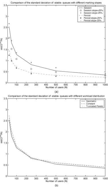
Fig. 1. Sample standard deviations of the normalized queue size from Monte Carlo simulations of the model. (a) Persistent flows versus session dynamics with different marking function slopes. (b) Different workload distributions.
with only persistent flows, i.e., flows with infinite workload. If the same parameter settings used with session dynamics are adopted, then the steady-state queue size becomes larger since all users are always active with persistent flows. As we are interested in the magnitude of queue oscillations (more specifi-cally, the SD of the queue oscillations), we need to maintain the same steady-state queue size to make a fair comparison with and without session dynamics. To this end, we adopt the same parameter settings used with session dynamics and increase the normalized capacity per user to 1.0 packet/user. This yields the same steady-state queue size of 5.1 packets/user for
.
Fig. 1(a) shows the simulation results comparing the sample SDs between these two setups. As expected from Theorem 2, the standard deviation decreases as for large values of in all of the simulations. It is clear from Fig. 1(a) that a major contribution to the random queue fluctuations comes from the session dynamics. Furthermore, as suggested earlier from the
Delta method, the magnitude of the queue fluctuations increases with the slope of the marking function. While the changes in the slope of the marking function have minimal effects on the SD in the system with only persistent flows (as long as the queue is stable), the SD of random queue fluctuations becomes much more sensitive to the slope of the marking function with session dynamics.
2) Effects of Different Workload Distributions: In this sub-section, we investigate the effects of different workload distribu-tions on the magnitude of random queue fluctuadistribu-tions. To this end we simulate the system with session dynamics under the same settings except for the workload distribution . We have set to be: 1) truncated Pareto and 2) constant workload in addition to the geometric distribution used in the previous subsection. We keep fixed at 400 packets for all distributions, and, hence, the steady-state queue size remains at 5.1 packets/user as the steady-state queue size depends only on the mean work-load as shown in (22). For truncated Pareto distribution,9 the
shape parameter is set to be 1.7 and the location parameter, i.e., the minimum size of the workload, is set to be 250 packets. For constant workload, a new connection has a fixed workload of 400 packets.
Fig. 1(b) shows the simulation results comparing the sample SDs with these workload distributions. Our results suggest that the workload distribution does not significantly alter the magni-tude of random queue fluctuations.
B. NS-2 Simulations
In this subsection, we verify the observations in the numer-ical examples in the previous subsection using a more realistic event-driven NS-2 simulator. In the simulations, we first grad-ually vary the number of sessions from 25 to 1000, and ob-serve the SD of the normalized queue fluctuations under similar setups as in the previous subsection.
The parameters used in the simulation with session dy-namics are given as follows. The bottleneck link capacity is Mb/s, and the buffer size is set to packets. The RED gateway with ECN option is configured with the marking function similar to the ones in Section VIII-A. Packet size is fixed to 1000 bytes, and the receiver advertised window size is set to 64 packets. The exponential averaging weight of the RED gateway is configured to be in order to have a similar time constant regardless of the number of users. A new connection generates a workload according to either a geometric, truncated Pareto, or constant distribution with the same mean of 400 packets. The rest of the parameters are set to similar values as in Section VIII-A. An idle period of a user be-tween two consecutive connections is exponentially distributed with a mean of 5 seconds. A connection terminates when it runs out of data to transfer. We also enable the drop_front_
9For Pareto distribution, the cumulative distribution function isF (x) = 1 0
(k=x) ,x k, where > 0is the shape parameter andk > 0is the location parameter, i.e., the minimum value of the rv with such distribution. With the shape parameter between(1; 2), the distribution is heavy-tailed, i.e., it has a finite mean but infinite variance. The truncated Pareto distribution limits the maximum value of the distribution and is often used to model the workload distribution of the objects transferred in the Internet for some 2 (1; 2)[3]. One can also specify the truncated Pareto distribution by specifying the shape, location, and the mean value.
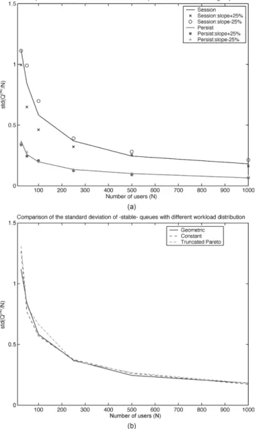
Fig. 2. Sample standard deviations of the normalized queue size from NS-2 simulations. (a) Persistent flows versus session dynamics with different marking function slopes. (b) Different workload distributions.
option of the RED mechanism so that the RED gateway marks the packet at the front of the queue rather than the packet that has just arrived. This reduces the feedback delay to the TCP senders. The round-trip propagation delays of the users are randomly selected uniformly from [50, 150] ms, with a mean of 100 ms. Under these parameters, the queue appears stable and the steady-state queue size is around 5 packets/user for
.
For the system with persistent TCP flows of infinite traffic, the same parameter values are adopted again, except for the ca-pacity being scaled up to Mb/s to maintain the same normalized steady-state queue size. In all of the simulations the queue is sampled every 100 ms, and the simulation time is 1000 seconds. We conduct 10 independent simulation runs for each setup. The sample SD is calculated by taking the average of 10 runs after discarding the first 100 seconds from each run, which is sufficient for the queue size to settle down to near steady-state. Fig. 2 shows the NS-2 simulation results. It is clear that the numerical results follow a similar trend as in the Monte Carlo
simulations of the model in the previous subsection. This sug-gests that our stochastic model captures the essential qualita-tive behavior of queue dynamics of an ECN/RED gateway. The SDs of the stochastic model from the Monte Carlo simulations are somewhat larger than those from the NS-2 simulation. This is partially an artifact of the discrete-time model as all packet transmissions from a connection in a RTT take place in a single timeslot in our model (as assumed in Section III). Furthermore, all the flows are synchronized at the timeslot level (at the be-ginning of each timeslot), whereas in the NS-2 simulations the flows are not synchronized with respect to any time scale and react to the marks from the RED gateway in an asynchronous manner (hence, the aggregate traffic is smoother).
C. Discussion
There are several observations one can make from both Monte Carlo and NS-2 simulations. First, it is clear that the arrivals and departures of connections (or simply session dynamics) are a major contributor to the random queue fluctuations. This is in part due to the aggressive behavior of the slow-start mechanism of TCP that causes bursty traffic arrival, combined with the fact that RED is not aimed at controlling short bursty flows by de-sign [5], [7]. Second, the magnitude of the random queue fluc-tuations isnotsensitive to the slope of the marking function. However, thestability of a system with TCP flows and RED gateway(s) is shown to be relatively sensitive to the slope of the system [6], [15], and, hence, a proper selection of the marking function is important from the viewpoint of maintaining a stable system. Third, oscillations caused by components (i), (ii), and (iv) are also significant. Hence, it may be possible to consid-erably reduce the queue oscillations by reducing these compo-nents through more fine-grained feedback information and/or a modification of TCP protocol.
Finally, the magnitudes of random fluctuations are not sensi-tive to the workload distribution. This observation may be some-what surprising at first as there are reports and analytical re-sults suggesting that heavy-tailed file size distributions (such as Pareto distribution) are a cause of the self-similar behavior of Internet traffic, leading to the heavy-tailed distribution of a bot-tleneck queue size (see [13] for examples). We note, however, that such observations are collected before AQM mechanisms such as RED are being widely-adopted, and the analytical re-sults suggesting the heavy-tailed distribution of queue size are carried out in the context of queue with infinite buffer and no in-teraction of TCP with an AQM mechanism. Our observation can be explained by the following arguments. In a stable TCP/AQM network, the AQM mechanism attempts to maintain a queue size around the stable operating point by regulating the TCP traffic. Hence, as long as there is sufficient TCP traffic, a stable network with an AQM mechanism will be able to successfully regulate the incoming traffic and, hence, the dynamics of the queue will not be sensitive to the workload distribution.
IX. CONCLUSION
In this paper, we have developed a scalable model of a RED gateway under a large number of TCP flows. We have demonstrated several interesting behaviors of the limiting
model. These results are further strengthened by our CLT results. They provide us with a scalable tool that can be utilized for network dimensioning without suffering from the curse of dimensionality. Furthermore, their proofs provide valuable insights into the queue behavior and help us design better AQM mechanisms. Our model is shown to be consistent with other previously proposed models in their respective regime. A formula for computing the average queue size in steady-state as a function of system parameters is derived and validated through numerical examples. The approach taken in this paper is extended to a generic probabilistic AQM mechanism and a congestion control mechanism in [19].
This research complements the control-theoretic studies of TCP/RED dynamics which derive sufficient conditions for the stability of the system that will ensure that the user rates and queue size asymptotically settle to equilibrium values. Under these sufficient conditions, Assumption (A3), i.e., , is reasonable. Therefore, the average behavior of such a complex stochastic feedback system at the equilibrium can be described using the LLNs, CLT, and the steady-state analysis when there is a large number of flows and the control parameters are set properly using the sufficient conditions for stability from the control-theoretic analyzes.
ACKNOWLEDGMENT
The authors would like to thank Prof. A. M. Makowski and Prof. S. H. Low for their helpful discussions and comments.
REFERENCES
[1] E. Altman, K. Avrachenkov, and C. Barakat, “TCP in presence of bursty losses,” inProc. ACM SIGMETRICS, Santa Clara, CA, 2000, pp. 124–133.
[2] F. Baccelli, D. R. McDonald, and J. Reynier, “A mean-field model for multiple TCP connections through a buffer implementing RED,” INRIA, Sophia Antipolis, France, Tech. Rep., Apr. 2002.
[3] M. E. Crovella and A. Bestavros, “Self-similarity in World Wide Web traffic: evidence and possible causes,” inProc. ACM SIGMETRICS, Philadelphia, PA, 1996, pp. 160–169.
[4] A. Durresi, M. Sridharan, C. Liu, M. Goyal, and R. Jain, “Multilevel early congestion notification,” inProc. 5th World Multiconf. Systemics, Cybernetics and Informatics, Orlando, FL, Jul. 2001, pp. 12–17. [5] S. Floyd and V. Jacobson, “Random early detection gateways for
con-gestion avoidance,”IEEE Trans. Netw., vol. 1, no. 4, pp. 397–413, Aug. 1993.
[6] C. V. Hollot, V. Misra, D. Towsley, and W.-B. Gong, “A control theoretic analysis of RED,” inProc. IEEE INFOCOM, Apr. 2001, pp. 1510–1519. [7] C. V. Hollot, Y. Liu, V. Misra, and D. Towsley, “Unresponsive flows and AQM performance,” inProc. IEEE INFOCOM, Apr. 2003, pp. 85–95. [8] V. Jacobson, “Congestion avoidance and control,” inProc. ACM
SIG-COMM, Aug. 1988, pp. 314–332.
[9] A. Kherani and A. Kumar, “Stochastic models for throughput analysis of randomly arriving elastic flows in the Internet,” inProc. IEEE IN-FOCOM, 2002, pp. 1014–1023.
[10] M. Mathis, J. Semske, J. Mahdavi, and T. Ott, “The macroscopic behavior of TCP congestion avoidance algorithm,”Comput. Commun. Rev., vol. 27, no. 3, pp. 67–82, Jul. 1997.
[11] M. Mellia, I. Stoica, and H. Zhang, “TCP model for short lived flows,”
IEEE Commun. Lett., vol. 6, no. 2, pp. 85–87, Feb. 2002.
[12] J. Padhye, V. Firoiu, D. Towsley, and J. Kurose, “Modeling TCP Reno performance: a simple model and its empirical validation,”IEEE/ACM Trans. Netw., vol. 8, no. 2, pp. 133–145, Apr. 2000.
[13] K. Park and W. Willinger, Eds.,Self-Similar Network Traffic and Perfor-mance Evaluation. New York: Wiley, 2000.
[14] V. Paxson and S. Floyd, “Wide area traffic: the failure of Poisson mod-eling,”IEEE/ACM Trans. Netw., vol. 3, no. 3, pp. 226–244, Jun. 1995. [15] P. Ranjan, E. H. Abed, and R. J. La, “Nonlinear instabilities in
TCP-RED,”IEEE/ACM Trans. Netw., vol. 12, no. 6, pp. 1079–1092, Dec. 2004.
[16] S. Shakkottai and R. Srikant, “How good are deterministic fluid models of Internet congestion control?,” inProc. IEEE INFOCOM, Jun. 2002, pp. 497–505.
[17] P. Tinnakornsrisuphap and R. J. La, “Asymptotic behavior of heteroge-neous TCP flows and RED gateways,” Inst. Syst. Res., Univ. Maryland, College Park, MD, Tech. Rep., 2003.
[18] P. Tinnakornsrisuphap and R. J. La, “Limiting model of ECN/RED under a large number of heterogeneous TCP flows,” Inst. Syst. Res., Univ. Maryland, College Park, MD, Tech. Rep., 2003.
[19] P. Tinnakornsrisuphap and R. J. La, “Characterization of queue fluctua-tions in probabilistic AQM mechanisms,”ACM SIGMETRICS Perform. Eval. Rev., pp. 283–294, Jun. 2004.
[20] P. Tinnakornsrisuphap and A. M. Makowski, “Limit behavior of ECN/RED gateways under a large number of TCP flows,” inProc. IEEE INFOCOM, Apr. 2003, pp. 873–883.
[21] A. W. van der Vaart,Asymptotic Statistics. Cambridge, U.K.: Cam-bridge Univ. Press, 1998.
[22] L. Zhang, S. Shenker, and D. Clark, “Observations on the dynamics of a congestion control algorithm: the effects of two-way traffic,” inProc. ACM SIGCOMM, Sep. 1991, pp. 133–145.
Peerapol Tinnakornsrisuphap (S’98–M’05) received the B.Eng. degree from Chulalongkorn University, Thailand, the M.S. degree from the University of Wisconsin-Madison, and the Ph.D. degree from the University of Maryland, College Park, in 1998, 2000, and 2004, respectively, all in electrical engineering.
He is a Senior Systems Engineer in Corporate Research and Development, Qualcomm, Inc., San Diego, CA. His research interests include resource allocation and congestion control in both wireline and wireless networks, end-to-end application performance, and queueing theory.
Richard J. La(S’98–M’01) received the B.S.E.E. degree from the University of Maryland, College Park, in 1994, and the M.S. and Ph.D. degrees in electrical engineering from the University of Cali-fornia at Berkeley in 1997 and 2000, respectively.
From 2000 to 2001, he was a Senior Engineer in the Mathematics of Communication Networks group at Motorola. Since August 2001, he has been on the faculty of the Department of Electrical and Computer Engineering, University of Maryland, College Park. His research interests include resource allocation in communication networks and application of game theory.
Dr. La is a recipient of a National Science Foundation (NSF) CAREER Award.