Anomaly Detection using a Convolutional Winner-Take-All Autoencoder

Anomaly Detection using a Convolutional

Winner-Take-All Autoencoder

We propose a method for video anomaly detection using a winner-take-all convolu-tional autoencoder that has recently been shown to give competitive results in learning for classification task. The method builds on state of the art approaches to anomaly detection using a convolutional autoencoder and a one-class SVM to build a model of normality. The key novelties are (1) using the motion-feature encoding extracted from a convolutional autoencoder as input to a one-class SVM rather than exploiting reconstruc-tion error of the convolureconstruc-tional autoencoder, and (2) introducing a spatial winner-take-all step after the final encoding layer during training to introduce a high degree of sparsity. We demonstrate an improvement in performance over the state of the art on UCSD and Avenue (CUHK) datasets.

1

Introduction

Anomaly detection in video surveillance has received increasing attention in recent years due to the growing importance of public security and safety [2,5,8,15, 21]. The wide range of application contexts, complexity of dynamic scenes and variability in anomalous behaviours makes anomaly detection a challenging task. It motivates the search for more effective methods for both feature representation and normality modelling.

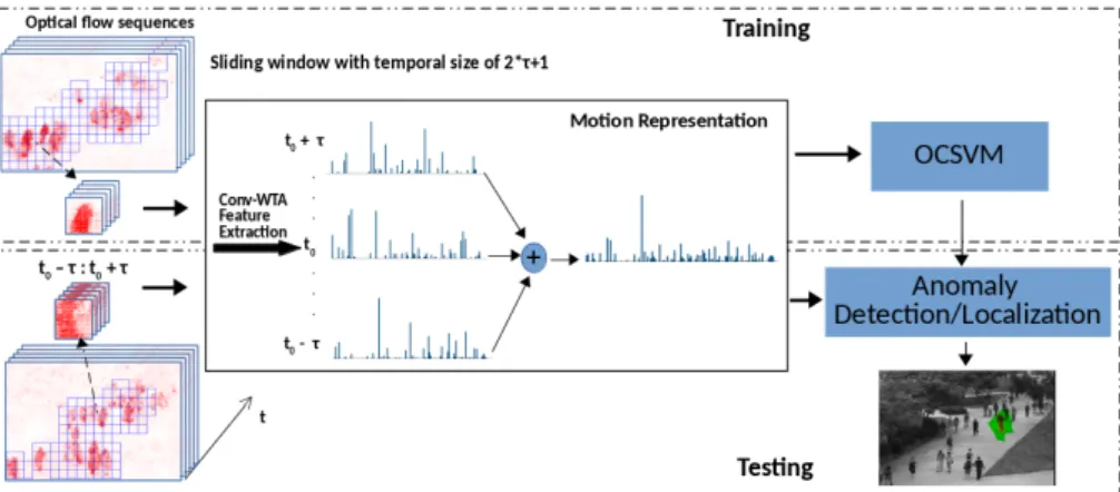
In this paper, we use a convolutional autoencoder and one-class SVM approach (Fig.

1) for anomaly detection. We demonstrate a significant improvement on state of the art performance by introducing a winner-take-all sparsity constraint on the autoencoder that has been used previously for object recognition [16]. We also use local normality modelling in which the field of view is partitioned into regions and one-class SVM is independently used within each region. Moreover, we only use optical flow data as input, instead of the combination of optical flow and appearance that has been used previously [8,21].

The rest of the paper is organised as follows. In Sect. 2 we review related work on anomaly detection using both motion features and deep architectures. In Sect. 3we outline our method, starting with the extraction of foreground patches (Sect. 3.1) and the genera-tion of a robust mogenera-tion-feature representagenera-tion (Sect. 3.2and3.3). These motion features are then used for anomaly detection with a one-class SVM (Sect. 3.4). Performance eval-uation is covered in Sect. 4and compared to the state of the art. Our experiments on two

c

2017. The copyright of this document resides with its authors. It may be distributed unchanged freely in print or electronic forms.

Figure 1: Overview of the method using a spatial sparsity Convolutional Winner-Take-All autoencoder for anomaly detection.

challenging datasets (UCSD [15] and Avenue [14]) show that our deep motion feature repre-sentation outperforms that of [8,21] and is competitive with the state of the art hand-crafted representations [5,14,20].

2

Related work

Most video based anomaly detection approaches involve a feature extraction step followed by model building. The model is often based on hand-crafted features extracted from low-level appearance and motion cues, such as colour, texture, and optical flow. Any occurrence that is an outlier with respect to the learnt model is regarded as an anomaly. Many different motion representations using dense optical flow or some other form of spatio-temporal gra-dients [2,11,17] have been proposed. In particular, the probability of optical flow patterns in local regions can be learnt using histograms [2]. Using the same low-level feature, Kim and Grauman [11] model local optical flow patterns with a mixture of probabilistic Princi-pal Component Analysis (MPPCA) models, and infer probability functions over the whole optical flow field using a Markov Random Field (MRF). Mehranet al. [15] also concen-trate on learning a representation which jointly models appearance and motion in crowded scenes and use it to detect both temporal and spatial anomalies. Also focusing on motion representation, Siqiet al. [20] propose a Spatially Localized Histogram of Optical Flow (SL-HOF) descriptor to encode the structure and local motion information of foreground objects in video. The authors show that this descriptor combined with one-class SVM modelling outperforms other common video descriptors (MHOF [5], 3D Gradient [14], 3D HOG, 3D HOF+HOG). All of these methods can do both anomaly detection and localization. Anoma-lous behaviour of crowds can also be detected by modelling the normal interactions between individuals using a social force model [17,19]

Several methods use reconstruction error as a metric for anomaly detection [5,14]. This follows the intuition that a normal event is likely to generate sparse reconstruction coeffi-cients with a small error, while the abnormal event generates a dense representation with a large reconstruction error. To detect anomalies at different scales and locations, Conget al. [5] propose several spatial-temporal structures, represented by a normalized Multi-scale

Histogram of Optical Flow. Their method can be extended to online event detection by an incremental self-update mechanism. However, the disadvantage of sparse coding is that an optimization step is required in both training and testing phases. A similar idea is found in [14], where the processing cost was decreased significantly using Sparse Combination Learning (SCL). Instead of coding sparsity using a whole dictionary, they code it directly as a set of possible combinations of basis vectors. Each combination corresponds to a set of dictionary atoms. With the learnt sparse combinations, for each testing feature, they only need to find the most suitable combination by evaluating the least squares error under the upper bound. This learning combination on 3D gradient features reaches a high detection rate.

Recently, deep learning architectures have been successfully used to tackle various com-puter vision tasks, such as object classification [10,12], object detection and semantic seg-mentation [7]. Inspired by these successes, Xuet al. [21] build a deep network based on a stacked de-noising autoencoder to learn appearance and motion features for anomaly detec-tion. Three feature learning pipelines for appearance representation, motion representation and joint appearance-motion representation are used. The third pipeline combines image pixels with optical flow to learn a joint representation. For abnormality detection, the late fusion is used to combine the abnormality scores predicted by three one-class SVM clas-sifiers on three learnt feature representations. Hasanet al. [8] compute a regularity score from a reconstruction error and use it as a metric for anomaly detection. However, a fully connected autoencoder and a fully convolutional autoencoder are used instead of the sparse coding method [5,14]. The learnt autoencoder reconstructs a normal motion with low error and creates higher reconstruction error for an irregular motion. The authors train their mod-els on multiple datasets and show that this generalises well to other datasets. However, this method does not localize an anomaly in a frame.

In this paper, we use a convolutional autoencoder to learn local flow features, but instead of applying across the whole field of view (FoV) [8], we apply within fixed-size windows onto the FoV. In [8], max-pooling is used to force compression of the flow field. With smaller windows, we are able to use Winner-Take-All (WTA) to produce a sparse (and com-pressive) representation as in [16]. This sparse representation promotes the emergence of distinct flow-features during training. Our motivation was to see whether the competitive performance using WTA obtained in [16] could be replicated for anomaly detection. Sim-ilar to [21], we use an autoencoder with fixed-size windows onto the FoV, coupled with a One-Class SVM (OCSVM) for anomaly detection. However, their autoencoder is fully con-nected and therefore learns larger flow features. By using a convolutional autoencoder within the window, coupled with a sparsity operator (WTA), we learn smaller generic flow-features that are potentially more discriminative for the OCSVM.

3

Our method

3.1

Extracting foreground patches

In common with recent approaches to anomaly detection [5,11,20], we look for anomalies via dense optical flow fieldsVt _{computed from successive pairs of video frames [13]. We}

assume that anomalies will only be found where there is non-zero optical flow in the image plane. Thus, we do not attempt to detect anomalous appearances of static objects. Patches are extracted by a moving window (48×48 for training the auto-encoder; 24×24 for training the

(a) (b)

Figure 2: Foreground patches extraction using a sliding window and thresholding of accumu-lated optical flow squared magnitude. (a) Video frame at timet. (b) Map of flow magnitude (from framestandt+1) with overlapping foreground patches superimposed; the red square delineates a single 24×24 foreground patch.

Figure 3: The architecture for a Conv-WTA autoencoder with spatial sparsity for learning motion representations.

one-class SVMs and in testing) with 50% overlap. Those patches with accumulated optical flow squared magnitude above a fixed threshold (empirically set at 10 in our experiments) are foregrounded for further processing; other patches are discarded. Figure2depicts the result of extracting foreground patches. This process is designed to eliminate most of the background, thereby reducing the computational cost of further processing.

3.2

Convolutional Winner-Take-All autoencoder

The Convolutional Winner-Take-All Autoencoder (Conv-WTA) [16] is a non-symmetric au-toencoder that learns hierarchical sparse representations in an unsupervised fashion. The encoder typically consists of a stack of several ReLU convolutional layers with small filters and the decoder is a linear deconvolutional layer of larger size. A deep encoder with small filters incorporates more non-linearity and effectively regularises a larger filter (e.g 11×11) by expressing as a decomposition of smaller filters (e.g. 5×5) [18]. Like [16], we use an autoencoder with three encoding layers and a single decoding layer (Fig. 3), giving a pipeline of tensorsHl_×Wl_×Cl_{, with the input layer being an input foreground patchPof}

optical flow vectors of sizeH0×W0×C0, whereC0=2. Zero-padding is implemented in all convolutional layers, so that each feature map has the same size as the input.

Given a training set withNforeground patches{Pn}_nN=1, the weightsWland biasesblof

each layerlare learnt by minimising the regularised least squares reconstruction error: 1 2N N

∑

∑

(a) (b)

Figure 4: Learnt deconvolutional filters of Conv-WTA trained on the UCSD Ped1 and Ped2 optical flow foreground patches: (a) visualisation of 128 filters, where flow-vector angle and magnitude is represented by hue and saturation [3] of 128 filters and (b) displacement vector visualisation of four filters (the 1st(top-left), the 6th(top-right), the 7th(bottom-left) and the 12th(bottom-right) filter in the first row of (a)).

wherek.kF denotes the Frobenius norm, ˆPnis the reconstruction of a patchPn. The

regu-larization termλ is a hyper-parameter used to balance the importance of the reconstruction

error and the weight regularization.

In the feedforward phase, after computing the encoding tensors3(x,y,c)(i.e. the output of f3in Fig.3), a spatial sparsity mapping is applied:

g_s3(x,y,c)=

(

s3(x,y,c), ifs3(x,y,c) =maxx0_,y0(s3(x0,y0,c))

0, otherwise (2)

where(x,y,c)are the row, column and channel indices of an element in the tensor. The resultgs3(x,y,c)has only one non-zero value for each channel. Thus, the level of sparsity is

determined by the number of feature maps (C3for the third layer). Only the non-zero hidden units are used in back-propagating the error during training.

3.3

Max pooling and temporal averaging for motion feature

representation

After training the autoencoder, the output of the third layer can be used as a feature represen-tation. C3non-zero activations in the encoding tensor correspond to deconvolutional filters (shown in Fig.4) which contribute in the reconstruction of each optical flow patch. Using the full output tensor of sizeH3×W3×C3as a motion feature representation preserves all of the information, but is very large. Therefore, we extract a sparse and compressed motion feature representation by turning off spatial sparsity and applyingmax-poolingon the last ReLU feature maps, over the spatial regionp×pwith stridep(denoted as Conv-WTA Feature Ex-traction in Fig.1). The max-pooling is only used following training of the autoencoder with WTA. Thus we benefit from the sparse representation that WTA promotes, whilst still reduc-ing the dimensionality of the codreduc-ing so that it is tractable for the OCSVM. Crucially, WTA preserves the location of the maximum response in each filter, which is critical to success-fully decoding and training the autoencoder to reduce reconstruction error. The location of the maximum response is less critical for anomaly detection and hence max-pooling, which greatly reduces dimensionality, is sufficient once training is complete.

Figure 5: Frame-level and pixel-level evaluation on the UCSD Ped1. The legend for the pixel-level (right) is the same as for the frame-level (left).

Figure 6: Frame-level and pixel-level evaluation on the UCSD Ped2.

To stabilise the output for eachH0×W0×C0foreground patch extracted at timet, we compute the motion feature representation at the same patch location over a temporal win-dow{t−τ:t+τ} (τ=2 in all experiments) and average the outputs. This gives a final

smoothed motion feature representation as output for each input foreground patch.

3.4

One class SVM modelling

One class SVM (OCSVM or unsupervised SVM) is a widely used method for outlier detec-tion. Given the final feature-based representations{d_i}M

i=1forM normal foreground optical

flow patches, we use OCSVM for learning a normality model. In the testing phase, the anomaly score of a foreground patch is calculated. For training the OCSVM, the meta-parameterν∈(0,1]determines the upper bound on the fraction of outliers and the lower

bound on the number of training examples used as support vectors. We employ a Gaus-sian kernelk(d,d0) =e−γkd−d0k2 for the SVM, in whichdandd0are the final feature-based representations of foreground patches.

In order to capture variations in normal flow patterns over the image plane, we divide the field of view intoI×Jregions. A separate OCSVM is learnt from the foreground patches located in each region. In testing, abnormality scores for each patch are generated from the OCSVM corresponding to the region within which that patch lies.

Method Ped1 Ped2 Frame level (%) Pixel level (%) Frame level (%) Pixel level (%) EER AUC EER AUC EER AUC EER AUC Sparse Coding [5] 19 86 54 46.1 - - - -Mixture Dynamic Texture [15] 25 81.8 55 44 25 85 55

-MPPCA [11] 40 59 82 - 30 77 -

-Social Force Model [17] 31 67.5 79 - 42 63 - -SCL [14] 15 91.8 40.9 63.8 - - - -SL-HOF [20] 18 87.5 35 64.4 9 95.1 19 81 AMDN [21] 16 92.1 40.1 67.2 17 90.8 - -Conv-AE [8] 27.9 81 - - 21.7 90 - -Conv-WTA + SVM[1×1] 27.9 81.3 46.8 56 8.9 96.6 16.9 89.3 Conv-WTA + SVM[6×9] 14.8 91.6 35.8 66.1 9.5 95 18.4 83.9 Conv-WTA + SVM[12×18] 15.9 91.9 35.7 68.7 11.2 92.8 21.2 80.9

Table 1: Performance comparison on UCSD Ped1 and Ped2.

4

Experimental evaluation

Dataset and Evaluation measures. We use two datasets (UCSD and Avenue) in our eval-uation. The UCSD dataset [15] contains two subsets of video clips, each corresponding to a different scene. The first one, denoted as Ped1, contains clips of 158×238 pixels and depicts a scene where groups of people walk toward and away from the camera. This subset contains 34 normal video clips and 36 video clips containing one or more anomalies for test-ing. The second, denoted as Ped2, has spatial resolution of 240×360 and contains scenes with pedestrian movement parallel to the camera plane. This contains 16 normal video clips, together with 12 test video clips. For our experiments on the UCSD dataset, we use ground-truth annotations from [15]. The Avenue dataset [14] contains 16 training videos and 21 testing videos. In total there are 15,328 training frames and 15,324 testing frames, all with resolution 360×640.

We evaluate the method using the frame-level and pixel-level criteria proposed by Weixin

et al. [15]. An algorithm classifies frames into those that contain an anomaly and those that do not. For both criteria, these predictions are compared with ground-truth to give the equal error rate (EER) and area under the curve (AUC) of the resulting ROC curve (TPR versus FPR) generated by varying an acceptance threshold. For a predicted anomalous frame to be correct, the pixel-level criterion [15] additionally requires that a ground-truth map of anomalous pixels is more than 40% covered by a map of predicted anomalous pixels. This criterion is well founded when the map of abnormal pixels is constrained to arise through thresholding a map of abnormality scores, as in [15]; otherwise it can be circumvented by setting every pixel in a frame as anomalous, when just one pixel is predicted to be anomalous - the frame-level score is not affected and the pixel-level criterion is always satisfied. In order to use the pixel-level criterion, we output a map of abnormality scores by bilinear interpolation of patch scores and evaluate our proposed method using this.

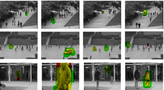
Figure 7: Detection results on the UCSD Ped1 (first row), the Ped2 (second row) and the Avenue dataset (third row). Our method detects the anomalies of a biker, skater, car and wheelchair on the UCSD dataset. Moreover, running, loitering, throwing object and jump-ing on the Avenue dataset are also detected. Pixels that have been correctly predicted as anomalous are shown in yellow; anomalous pixels that have been missed are shown in red, and pixels that have been incorrectly predicted as anomalous are shown in green.

Convolutional WTA autoencoder architecture and parameters. The Conv-WTA au-toencoder architecture is 128conv5-128conv5-128conv5-128deconv11 with a stride of 1, zero-padding of 2 in each convolutional layer and cropping of 5 in the deconvolutional layer. We train our model on 3×105foreground optical flow patches of size 48×48 extracted from the UCSD dataset, using stochastic gradient descent with batch sizeNb=100, momentum

of 0.9 and weight decayλ=5×10−4 [12]. The weights in each layer are initialized from a

zero-mean Gaussian distribution whose standard deviation is calculated from the number of input channels and the spatial filter size of the layer [9]. This is a robust initialization method that particularly considers the rectifier nonlinearities. The biases are initialized to zero. A fixed value for the learning rateα =10−4is used following the first iteration. We use the MatConvNet toolbox [1], augmented to perform WTA.

One class SVM model. The LIBSVM library (version 3.22) [4] was employed for our experiments. The parameterν is chosen from the range{2−12,2−11, . . . ,20}andγ (in the

Gaussian kernel) is from the range{2−12,2−11, . . . ,212}. Both parameters are selected by 10-fold cross validation on training data containing only normal activities.

For the UCSD dataset, we resize the frame resolution to 156×240. We evaluate perfor-mance with three subdivisions of the field of view: [1×1],[6×9]and[12×18]. The first of these is equivalent to operating over the entire field of view. For the Avenue dataset, we resize the frame resolution to 120×156 which is close to one scale used in [14]. Here we evaluate performance with three different subdivisions of the field of view: [1×1],[4×6]

and[8×12]. In both cases, the sub-divisions are chosen to divide at pixel boundaries. 10-fold cross validation is used once on each dataset for the SVM[1×1]model to select values for the parameters to be used in all experiments (ν=2−9andγ=2−7).

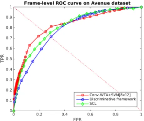
Figure 8: Frame-level comparison on the Avenue dataset.

Method Frame level (%) Pixel level (%)

EER AUC EER AUC

SCL [14]* - 80.9 - -Discriminative framework [6] - 78.3 - -Conv-AE [8] 25.1 70.2 - -Conv-WTA + SVM[1×1] 28.2 78.1 50 50.7 Conv-WTA + SVM[4×6] 26.5 81 45.7 54.2 Conv-WTA + SVM[8×12] 24.2 82.1 45.2 55

Table 2: Performance comparison on the Avenue dataset. (* the results from [6] replicated SCL method [14])

Comparison with the state of the art. In this section, we compare the proposed frame-work with state of the art methods on the UCSD and Avenue datasets. Each method is compared on both ROC curves (Fig.5,6and8) and the EER/AUC metric (Tables1,2). Our method achieves a significantly better EER and AUC result on Ped2 with SVM[1×1](Table

1) and on Avenue with SVM[8×12](Table2), where there is greater variation in depth. Moreover, the method obtains comparable results with SVM[6×9]on Ped1 (Table1).

As can be seen from Table1, a finer sub-division gives better results on Ped1, whereas the best results are obtained for no sub-division on Ped2 (i.e.[1×1]). This may be explained by the greater variation in scale in Ped1 than in Ped2, leading to substantial variations in the patterns of motion as an object moves in depth through the scene. It may also be due to ‘contextual’ anomalies such as a pedestrian walking over grass that occupies only a portion of the scene. Finally, it is worth noting that a finer sub-division results in less training data for each one-class SVM, which may result in unexpected results where there is inadequate training data. Figure7displays some detection results on the UCSD and the Avenue datasets.

Varying max-pooling size. Max-pooling is used after training the autoencoder with WTA. Thus, we benefit from the sparse representation that WTA promotes and the dimensionality reduction of the coding for OCSVM. In this section, we evaluate the impact use of max-pooling by varying the max-max-pooling area on Ped1 (Table3). We use the encoding part of the Conv-WTA autoencoder (removing zero-padding in convolutional layers and turning off spatial sparsity) to extract motion features from foreground patches of size 24×24. Then max-pooling is applied on the last ReLU tensor of size 12×12×128 with different area and

p=12 1×1×128 [6×9] 15.5 91.3 34.4 65.7 [12×18] 16.2 91.5 35.5 67.7 p=6 2×2×128 [1×1] 27.9 81.3 46.8 56 [6×9] 14.8 91.6 35.8 66.1 [12×18] 15.9 91.9 35.7 68.7 p=4 3×3×128 [1×1] 27.9 80.8 46.8 55.4 [6×9] 15.3 91.1 38.6 63.2 [12×18] 16.7 91.4 38.1 65.9

Table 3: Performance comparison on UCSD Ped1 with different kernel sizes and strides of max-pooling and different subdivisions.

stride. Table3shows a comparison on Ped1. The results are better with max-pooling size

p=6. This size is used for comparing our results with the state of the art on the UCSD dataset (Table1). We use max-pooling size p=12 for evaluating our frame-work on the Avenue dataset.

5

Conclusions

We present a framework that use a deep spatial sparsity Conv-WTA autoencoder to learn a motion feature representation for anomaly detection. The temporal fusion on feature space gives a robust feature representation. Moreover, the combination of this motion feature rep-resentation with a local application of one-class SVM gives competitive performance on two challenging datasets in comparison to existing state-of-the-art methods. There is potential to improve results further by adding an appearance channel alongside the optical flow chan-nel, and also capturing longer-term motion patterns using a recurrent convolutional network following on from the Conv-WTA encoding, and replacing our temporal smoothing.

References

[1] Matconvnet: Cnns for matlab.http://www.vlfeat.org/matconvnet/. [2] Amit Adam, Ehud Rivlin, Ilan Shimshoni, and Daviv Reinitz. Robust real-time unusual

event detection using multiple fixed-location monitors. IEEE transactions on pattern analysis and machine intelligence, 30(3):555–560, 2008.

[3] Simon Baker, Daniel Scharstein, JP Lewis, Stefan Roth, Michael J Black, and Richard Szeliski. A database and evaluation methodology for optical flow. International Jour-nal of Computer Vision, 92(1):1–31, 2011.

[4] Chih-Chung Chang and Chih-Jen Lin. Libsvm: a library for support vector machines.

[5] Yang Cong, Junsong Yuan, and Ji Liu. Sparse reconstruction cost for abnormal event detection. InComputer Vision and Pattern Recognition (CVPR), 2011 IEEE Confer-ence on, pages 3449–3456. IEEE, 2011.

[6] Allison Del Giorno, J Andrew Bagnell, and Martial Hebert. A discriminative frame-work for anomaly detection in large videos. InEuropean Conference on Computer Vision, pages 334–349. Springer, 2016.

[7] Ross Girshick, Jeff Donahue, Trevor Darrell, and Jitendra Malik. Rich feature hierar-chies for accurate object detection and semantic segmentation. InProceedings of the IEEE conference on computer vision and pattern recognition, pages 580–587, 2014. [8] Mahmudul Hasan, Jonghyun Choi, Jan Neumann, Amit K Roy-Chowdhury, and

Larry S Davis. Learning temporal regularity in video sequences. InProceedings of the IEEE Conference on Computer Vision and Pattern Recognition, pages 733–742, 2016.

[9] Kaiming He, Xiangyu Zhang, Shaoqing Ren, and Jian Sun. Delving deep into rectifiers: Surpassing human-level performance on imagenet classification. InProceedings of the IEEE international conference on computer vision, pages 1026–1034, 2015.

[10] Fu Jie Huang, Y-Lan Boureau, Yann LeCun, et al. Unsupervised learning of invariant feature hierarchies with applications to object recognition. InComputer Vision and Pattern Recognition, 2007. CVPR’07. IEEE Conference on, pages 1–8. IEEE, 2007. [11] Jaechul Kim and Kristen Grauman. Observe locally, infer globally: a space-time mrf

for detecting abnormal activities with incremental updates. InComputer Vision and Pattern Recognition, 2009. CVPR 2009. IEEE Conference on, pages 2921–2928. IEEE, 2009.

[12] Alex Krizhevsky, Ilya Sutskever, and Geoffrey E Hinton. Imagenet classification with deep convolutional neural networks. InAdvances in neural information processing systems, pages 1097–1105, 2012.

[13] Ce Liu. Beyond pixels: exploring new representations and applications for motion analysis. PhD thesis, Citeseer, 2009.

[14] Cewu Lu, Jianping Shi, and Jiaya Jia. Abnormal event detection at 150 fps in matlab. In

Proceedings of the IEEE International Conference on Computer Vision, pages 2720– 2727, 2013.

[15] Vijay Mahadevan, Weixin Li, Viral Bhalodia, and Nuno Vasconcelos. Anomaly detec-tion in crowded scenes. InComputer Vision and Pattern Recognition (CVPR), 2010 IEEE Conference on, pages 1975–1981. IEEE, 2010.

[16] Alireza Makhzani and Brendan J Frey. Winner-take-all autoencoders. InAdvances in Neural Information Processing Systems, pages 2791–2799, 2015.

[17] Ramin Mehran, Alexis Oyama, and Mubarak Shah. Abnormal crowd behavior de-tection using social force model. InComputer Vision and Pattern Recognition, 2009. CVPR 2009. IEEE Conference on, pages 935–942. IEEE, 2009.

International Conference on, pages 830–837. IEEE, 2011.

[20] Siqi Wang, En Zhu, Jianping Yin, and Fatih Porikli. Anomaly detection in crowded scenes by sl-hof descriptor and foreground classification.

[21] Dan Xu, Elisa Ricci, Yan Yan, Jingkuan Song, and Nicu Sebe. Learning deep rep-resentations of appearance and motion for anomalous event detection. arXiv preprint arXiv:1510.01553, 2015.