Universidade de São Paulo
2015-07
Effectiveness of random search in SVM
hyper-parameter tuning
International Joint Conference on Neural Network, 2015, Killarney.
http://www.producao.usp.br/handle/BDPI/49443
Downloaded from: Biblioteca Digital da Produção Intelectual - BDPI, Universidade de São Paulo
Biblioteca Digital da Produção Intelectual - BDPI
Effectiveness of Random Search in
SVM hyper-parameter tuning
Rafael G. Mantovani *, Andre L. D. Rossi t, Joaquin Vanschoren t, Bernd Bischl § and Andre C. P. L. F. de Carvalho * * Universidade de Sao Paulo (USP), Sao Carlos - SP, Brazil
Email: {rgmantov.andre}@icmc.usp.br
t Universidade Estadual Paulista (UNESP), Itapeva - SP, Brazil Email: [email protected]
t Eindhoven University of Technology (TV/e), Eindhoven, The Netherlands Email: [email protected]
§ Ludwig-Maximilians-University Munich, Germany Email: [email protected] Abstract-Classification is one of the most common machine
learning tasks. SVMs have been frequently applied to this task. In general, the values chosen for the hyper-parameters of SVMs affect the performance of their induced predictive models. Several studies use optimization techniques to find a set of hyper-parameter values that induces classifiers with good predictive performance. This paper investigates the hypothesis that a simple Random Search method is sufficient to adjust the hyper-parameters of SVMs. A set of experiments compared the performance of five tuning techniques: three meta-heuristics commonly used, Random Search and Grid Search. The experi mental results show that the predictive performance of models using Random Search is equivalent to those obtained using meta heuristics and Grid Search, but with a lower computational cost.
I. INTRODUCTION
Classification is one of the most common machine learning tasks, on Support Vector Machines (SVMs) have been suc cessfully used [1]. Despite their good predictive performance, SVMs are sensitive to the values of their hyper-parameters. Several studies investigate the use of optimization techniques to adjust these hyper-parameters in classification tasks [2] [4]. Most of these techniques investigate the employment of sophisticated meta-heuristics (MTHs), which usually present high computational costs.
Recent studies suggest that a less complex optimization technique, such as a Random Search (RS) may be sufficient for SVM hyper-parameters optimization [5]. SVMs have relatively few hyper-parameters, associated with the kernel functions chosen. Thus, this optimization is a problem of low dimen sionality that could be addressed by simple techniques. These few hyper-parameters are often dependent on each other [6], allowing the existence of a optimal region instead of a single global optimal solution. As a result, a simple method that perform few evaluations may efficiently find a good solution. In this study, we investigate the use of the RS method for adjusting the hyper-parameters of SVMs. We perform several experiments to see how RS affects the predictive performance of the induced SVM models. We expect that the models induced by SVMs tuned by a simple technique, like RS, can
978-1-4799-1959-8/15/$31.00 @2015 IEEE
have a predictive accuracy similar to models induced by more sophisticated techniques, such as MTHs. We also compare RS with another simple optimization technique with a higher computational cost: Grid Search (GS).
The experiments used a large number of data sets, and compared RS with three meta-heuristics conunonly used SVM hyper-parameter tuning: Genetic Algorithm (GA) [7], Particle Swarm Optimization (PSO) [8] and Estimation of Distribution Algorithms (EDA) [9]; and another optimization technique that uses a very simple heuristic, Grid Search (GS), as used by [10]. This paper is structured as follows: section II contextualizes the hyper-parameter tuning problem and cites some techniques explored by related work. Section III presents our experimental methodology and steps covered to evaluate these techniques. The results are discussed in section IV. The last section presents our conclusions and future work.
II. HYPER-PARAMETER TUNING
Obtaining a suitable configuration for the hyper-parameters of a ML algorithm requires specific knowledge, intuition and, often, trial and error. The tuning of these hyper-parameters is usually treated as an optimization problem [11], whose objec tive function captures the predictive performance of the model induced by the algorithm. For a given data set D, the optimal hyper-parameter configuration maximizes the performance of this algorithm in D. A common performance measure used in this context is the predictive accuracy. The tuning task has many aspects that can make it difficult:
• Hyper-parameter values that lead to a model with high predictive performance for a given data set may not lead to good results for other data sets;
• Hyper-parameter values often depend on each other. Hence, optimizing hyper-parameters independently is not a reasonable strategy;
• Evaluation of a specific hyper-parameter configura tion, let alone many, can be very time consuming. Many deterministic and probabilistic approaches have been proposed for the optimization of hyper-parameters of
classifi-cation algorithms [12]. Among the deterministic approaches, GS is one of the most used due to its simplicity and good results in previous studies. However, GS is an exhaustive search method that requires a discretization of the hyper parameters space. Some authors have explored more robust deterministic approaches [S]. Nevertheless, GS is still the most used method in the literature, since its computational demands can be satisfied in several cases [3].
For optimization of many hyper-parameters in large data sets, GS becomes computationally infeasible. In these sce narios, probabilistic optimization methods, such as GAs, are generally preferred. Some studies employ GAs to optimize hyper-parameters of Artificial Neural Networks (ANNs) or SVMs [13]. Other authors explored the use of Pattern Search (PS) [14] or techniques based on gradient descent [IS]. Several automated tools are also available in the literature, such as methods based on local search (ParamILS [16]), estimation of distributions (REVAC [17]) and Bayesian optimization (Auto Weka [18]).
In [S], the authors use RS to tune Deep Belief Net works (DBNs), comparing RS with grid methods. The authors showed empirically and theoretically that RS are more effi cient for hyper-parameter optimization than trials on a grid. Their experiments performed had tuned over 20 DBN hyper parameters. Other recent works use a collaborative solution
[19], or combine optimization techniques for tuning algorithms in computer vision problems [20].
A complete survey of RS methods for optimization prob lems can be found in [21]. The author reports several studies using RS algorithms (pure and adaptive) to solve discrete and continuous optimization problems. Theoretical results regard ing the convergence of these methods to a global optimum are also summarized. A limitation pointed out is that strong convergence to a global optimum requires strong assumptions on the structure of the problem.
III. MATERIALS AND MET HODS
As previously mentioned, we aim to investigate when a simple but faster technique, such as RS, should be used instead of a more sophisticated, but slower, approach for tuning SVM hyper-parameters. We employed simple search strategies (RS, GS) and MTHs (GA, PSO, EDA) to tune SVM hyper parameters for 70 different data sets. The accuracy was used to assess the predictive performance of the induced models and also to guide the search of the optimization techniques.
In this paper, we consider only the Gaussian kernel for SVMs. The choice of this kernel is due to its flexibility in different problems compared to other kernels [22]. Therefore, the simple search strategies and the MTHs have to tune the parameter cost (C) and gamma (,). The former is a parameter of the SVMs and the latter is the a parameter of the Gaussian kernel. Table I shows the range of values for C and, explored in this work [23].
In the MTHs, each individual is a pair of real values for
C and ,. The accuracy obtained by SVMs was used as the fitness value for all optimization techniques. Higher fitness values indicate more promising hyper-parameter values.
TABLE I. SY M HYPER-PARAMETERS RANGE VALUES INVESTIGATED
[23] . Hyper-parameter cost (C) gamma (,,) A. Experimental methodology Maximum
A few experimental methodologies to repeatedly select and assess regression and classification models can be found in the literature [24]. When a rigorous model comparison/evaluation is required, a nested cross-validation (N-CV) methodology is usually recommended to assess the performance of models. In this experimental methodology, each data set is divided into
kl partitions and each of these partitions is further divided into k2 partitions. The inner partition is used for assessing the average validation accuracy of each possible combination of values for C and, hyper-parameters (fitness value). The test accuracy is assessed for the data in the outer loop by using the best individual returned by the tuning technique for the inner loop.
This design minimizes the bias of the data when induc ing models, but has a high computational cost, since each technique is executed kl x k2 times to obtain a performance estimate. If data are divided into 10-folds in two loops, 100 models are induced to evaluate a single data set. The N CV design is used in a theoretical scenario, and may not be practical in real tasks, especially with hyper-parameter tuning. Thus, it is interesting to explore alternatives to minimize the bias in data sampling, and being faster than the N-CV.
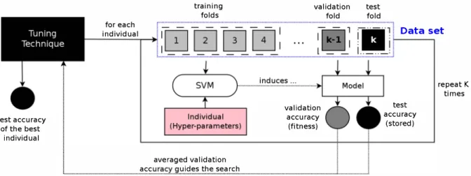
An alternative is to induce models in a single cross validation step (S-CV) separating data into training, validation and test partitions. The S-CV methodology is depicted in Figure 1. Whenever a tuning technique is executed, the data set is divided into k stratified partitions. SVM is trained with k -2
partitions (training folds) for each candidate solution found by the technique. One partition is separated to validate the model (validation fold) and the remaining partition is separated to test it (test fold).
The test and validation accuracies are assessed through the model induced with the training partitions and the hyper parameters values found by the optimization technique. This process is repeated for all k permutations in S-Cv. The average validation accuracy is then used as the fitness value of an individual of the MTHs, which will guide the search process. In the end, the individual with the highest validation accuracy is returned (with its hyper-parameters values), and the technique performance is the average test accuracy of this individual. We used this S-CV experimental methodology in this paper.
B. Data sets
Seventy data sets from the VCI repository [2S] were used in the experiments. All of them were preprocessed and standardized with f..l = 0 e (J = 1 internally when running in
SVMs, since this can reduce the time to find support vectors. This internal data normalization is performed by package 'el071' (R interface for 'LIBSVM' library), employed here to train SVMs.
test accuracy of the best individual for each individual acc training folds averaged validation uides the search . . . . . . . . . .
validation test validation accuracy (fitness) fold fold Data set test accuracy (stored) repeat K times
Fig. 1. Single cross-validation (S-CV) experimental methodology for hyper-parameter tuning.
In terms of data complexity, data sets may be categorized in two classes of problems:
• Low complexity: a data set that has less than 50 attributes. Most of the datasets are in this category
(65 of 70);
• High complexity: a data set that has 50 or more attributes. Only 5 of the all data sets are included here. The average number of features per data sets is 15, with a standard deviation of 17. As such, it should be noted that, in this work, optimization techniques are assigning solutions to problems of relatively low complexity.
C. Tuning techniques
The MTHs, namely GA, PSO and EDA were implemented in R using packages available on CRANI: "GA", "pso", and "copulaedas", respectively. The parameter values for GA and PSO were the same used in [23].
The GA uses: a uniform random mutation operator with a rate value of 0.05; a selection method by tournament (with k=3); and a local arithmetic crossover methodology. The chosen EDA was a Gaussian Copula EDA (GCEDA) with the default parameters provided by the package. GCEDA assumes that there are dependence relationship between variables.
The simpler search techniques, GS and RS, were im plemented. Moreover, we compared SVMs with the hyper parameter default values (DF) provided by the package 'e1071'
[26]. Each technique was run 30 times for each data set, because all techniques are stochastic (except GS). For each candidate solution, we calculated the mean validation and test predictive accuracy, together with the standard deviation.
IV. EXPERIMENT S
The first step in the experiments was the definition of how many hyper-parameter settings should be analyzed by the techniques. As such, we investigated whether increasing the number of evaluations (individuals in the case of MTHs) leads to a higher accuracy of the induced models.
I http://cran.r-project.org/
TABLE II. SV M HYPER-PARAMETERS SCENARIOS INVESTIGATED.
Scenario Evaluations Pop Size Generations
sc-200 200 20 10
sc-2.Sk 2S00 100 2S sc-Sk SOOO 100 50 sc-IOk 10000 100 100
Since we just want a simpler estimate, we used only 22 data sets (a heterogeneous control group) and the GA. Four combinations of numbers of individuals in the population and maximum number of generations were considered, which are illustrated in Table II.
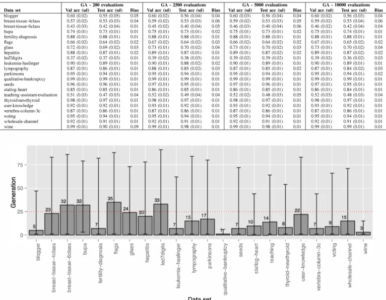
The experimental results are summarized in Table III. The first column presents the data sets used in this experiment. The next columns are the validation and test accuracies for each combination, including the bias (the difference between these accuracies). These values are averaged over 30 runs, with the standard deviation in parenthesis.
According to these results, the evaluation of a larger num ber of individuals with more generations did not improve the predictive accuracy. Similar accuracy values (both validation and test) were obtained in all combinations, with a low standard deviation associated with the induced models. The biases calculated are also very small even in combinations with fewer evaluations. A possible reason is the small number of hyper-parameters in this study and the simple landscape of the solutions. Therefore, we decided to use the smallest number of evaluations in the next experiment.
A. Comparison of tuning strategies
In order to illustrate the behaviour of the tuning in these different scenarios, we generated graphics for all data sets from control group. Figure 3 show graphics of the 'led7digit' data set. These pictures illustrate the area covered by the GA for the SVM hyper-parameter search space, and the histogram of the accuracies of the induced models during the search process.
Figures left-sided (3a, 3c, 3e, 3g) show the heat map of the individuals found during the GA execution. Each point represents a solution in the hyper-parameter space. Red points represent better predictive accuracy, while yellow represent lower accuracy. The black point represents hyper-parameter
Data set blogger breast-tissue-4c1ass breast-tissue-6c1ass bupa fertility-diagnosis flags glass hepatitis led7digits leukemia-haslinger Iympography parkinsons qualitative-bankruptc y seeds statlog-heart teaching- assistant-evaluation thyroid-newthyroid user-knowledge veI1ebra-c olumn-3c voting wholesale-channel wine 75 -Q; Cl 8' :c .� r- �--I (J) gj (j ,. CD " gj
1
gj � .0TABLE III. SY M ACCURACIES OF THE INDUCED MODELS OBTAINED IN EACH SCENARIO. GA -200 evaluations GA -2500 evaluations GA -5000 evaluations
Val ace (sd) 0.60 (0.02) 0.57 (0.02) 0.43 (0.03) 0.74 (0.01) 0.88 (0.01) 0.66 (0.02) 0.72 (0.01) 0.88 (0.01) 0.37 (0.02) 0.90 (0.01) 0.87 (0.01) 0.95 (0.01) 0.99 (0.01) 0.96 (0.01) 0.85 (0.01) 0.51 (0.03) 0.98 (0.01) 0.92 (0.01) 0.87 (0.01) 0.95 (0.01) 0.92 (0.01) 0.99 (0.01) 32 32 .. . . .. .. I (J) OS gj 0. " (j .0 co I CD " gj
1
gj � .0Test ace (sd) Bias Val ace (sd) Test ace (sd) Bias Val ace (sd) Test ace (sd)
... 7 r-0.55 (0.05) 0.05 0.60 (0.02) 0.53 (0.03) 0.04 0.59 (0.02) 0.42 (0.04) 0.01 0.45 (0.02) 0.73 (0.01) 0.01 0.75 (0.01) 0.88 (0.01) 0.01 0.88 (0.01) 0.64 (0.02) 0.02 0.67 (0.02) 0.69 (0.02) 0.03 0.73 (0.01) 0.87 (0.01) 0.02 0.89 (0.01) 0.37 (0.03) 0.01 0.39 (0.02) 0.89 (0.01) 0.01 0.90 (0.01) 0.86 (0.01) 0.01 0.88 (0.01) 0.94 (0.01) 0.01 0.95 (0.01) 0.99 (0.01) 0.01 0.99 (0.01) 0.96 (0.01) 0.01 0.97 (0.01) 0.85 (0.01) 0.01 0.86 (0.01) 0.47 (0.03) 0.04 0.52 (0.02) 0.97 (0.01) 0.01 0.98 (0.01) 0.92 (0.01) 0.01 0.93 (0.01) 0.86 (0.01) 0.01 0.87 (0.01) 0.94 (0.01) 0.01 0.95 (0.01) 0.91 (0.01) 0.01 0.92 (0.01) 0.90 (0.01) 0.09 0.99 (0.01) 35 33 --r- r-24 . . .. .. . .� �" 20"' . . .. ... ---,
�J[D
I I I (J) (J) (J) (J) !!l '0;�
gj E 'c, 0 Oi c: c;, '5 Cl 0. r--OS CD �'9
.r: � :.e .l!! 0.56 (0.04) 0.53 (0.03) 0.40 (0.04) 0.73 (0.01) 0.88 (0.01) 0.64 (0.02) 0.70 (0.02) 0.87 (0.01) 0.38 (0.03) 0.88 (0.02) 0.85 (0.02) 0.94 (0.01) 0.99 (0.01) 0.95 (0.01) 0.85 (0.01) 0.49 (0.04) 0.97 (0.01) 0.92 (0.01) 0.86 (0.01) 0.94 (0.01) 0.91 (0.01) 0.98 (0.01) ... . . ... . ... 15 7 17 0.04 0.06 0.05 0.02 0.01 0.03 0.04 0.01 0.01 0.02 0.03 0.01 0.01 0.01 0.01 0.04 0.01 0.01 0.01 0.01 0.01 0.01 · · · 1 · · 0.60 (0.03) 0.59 (0.02) 0.46 (0.03) 0.75 (0.01) 0.88 (0.01) 0.66 (0.02) 0.73 (0.01) 0.89 (0.01) 0.39 (0.02) 0.90 (0.01) 0.87 (0.01) 0.95 (0.01) 0.99 (0.01) 0.97 (0.01) 0.86 (0.01) 0.52 (0.02) 0.98 (0.01) 0.93 (0.01) 0.87 (0.01) 0.95 (0.01) 0.92 (0.01) 0.99 (0.01) 7 0.56 (0.04) 0.53 (0.03) 0.40 (0.04) 0.73 (0.01) 0.88 (0.01) 0.64 (0.02) 0.70 (0.02) 0.87 (0.02) 0.39 (0.02) 0.89 (0.01) 0.85 (0.01) 0.94 (0.01) 0.99 (0.01) 0.96 (0.01) 0.85 (0.01) 0.48 (0.03) 0.97 (0.01) 0.92 (0.01) 0.86 (0.01) 0.94 (0.01) 0.91 (0.01) 0.98 (0.01) . . . . r-nl. l
...!L
�,�
I I I I I Q; ,., Cl .r:�
c: � OS 8' .r: 0. � E 'E CD � "'" " � (J) ,., (J) t:: Cl -c c: " -g OS c:'[
0 a CD :2 (J) 5l .r: c: " aJ .r: .l2 I :;; c: Cl .l!l j iii os .Q CD 0. .0 I 19 c: I CD '" -c .� 'e Oi ,., .... £ 1i! " C" Data setFig. 2. Average generation that the best solution was found by data set
GA -10000 evaluations
Bias Val ace (sd) Test ace (sd)
0.04 0.60 (0.02) 0.56 (0.03) 0.05 0.59 (0.02) 0.53 (0.04) 0.06 0.46 (0.02) 0.42 (0.04) 0.02 0.75 (0.01) 0.74 (0.01) 0.01 0.88 (0.01) 0.88 (0.01) 0.02 0.67 (0.01) 0.65 (0.02) 0.03 0.73 (0.01) 0.70 (0.02) 0.02 0.89 (0.01) 0.87 (0.02) 0.01 0.39 (0.02) 0.36 (0.02) 0.01 0.90 (0.01) 0.89 (0.01) 0.02 0.87 (0.01) 0.84 (0.02) 0.01 0.95 (0.01) 0.94 (0.01) 0.01 0.99 (0.01) 0.99 (0.01) 0.01 0.97 (0.01) 0.95 (0.01) 0.01 0.86 (0.01) 0.84 (0.01) 0.05 0.52 (0.03) 0.48 (0.03) 0.01 0.98 (0.01) 0.97 (0.01) 0.01 0.93 (0.01) 0.92 (0.01) 0.01 0.87 (0.01) 0.86 (0.01) 0.01 0.95 (0.01) 0.94 (0.01) 0.01 0.92 (0.01) 0.91 (0.01) 0.01 0.99 (0.01) 0.99 (0.01) 22
1
15db
I I I I CD " Cl Qi CD Cl (') c: c: c: -g c: I ., S! c: os .��
E " .r: 'f .2�
CD .!. 0; 5l .0 os � (J) " CD .r: 0 t:: ;: � Bias 0.04 0.06 0.04 0.01 0.01 0.02 0.04 0.02 0.03 0.01 0.03 0.02 0.01 0.01 0.01 0.04 0.01 0.01 0.01 0.01 0.01 0.01default values. We can see that increasing the number of evaluations is possible to have a better idea of the search space and where the best solutions to the problem are located.
In Figure 2 are depicted the average generation where the best solutions were found by GA in the scenario with 10 thousand evaluations. The figure shows the values for each data set in the control group. It may be observed that, in some cases, the GA quickly found good solutions (about 3 to 5 generations). In other data sets, GA spent around 30 iterations to find the best solutions. However, most data sets can have a good convergence up to 25 generations (indicated by the dashed line). Therefore, we have chosen a maximum of 25 iterations for the tuning tasks.
The graphics on the right (3b, 3d, 3f, 3h) depict the accuracies obtained in validation and test sets. Bars in pink indicate the amount of individuals of the test set that reached a certain level of accuracy. The light blue bars denote those from the validation set. The region in gray is where the two distributions overlap. The more overlap, the lower the bias technique to estimate the performance of models in both evaluation sets.
When increasing the number of evaluations, the distribu tions of the accuracies tend to overlap and the bias in a S-CV decreases. However, there is a greater number of points that achieve the same accuracy. This can be observed mainly in executions up to 2000 evaluations. This behaviour can be seen by both the density of dots in the heatmaps and the amount of individuals with the same accuracy in histograms.
To perform well, EDAs need a population with at least
100 individuals [9]. So, we set the initial population of all optimization techniques to 100 individuals. Doing this leads to a total of at most 25 x 100 = 2500 evaluations of hyper
parameter values during the search. This value is in line with what was done in [1], where the authors executed a Genetic Prograrmning algorithm to adjust SVM hyper-parameters with a budget of 2000 evaluations.
0-� -5-� -10- -15- 0-� -5-� -10- -15- 0-� -5-� -10- -15- 0-� -5-� -10- -15-SVM hyper-parameters space 10 cost
(a) GA heatmap with 200 evaluations SVM hyper-parameters space
10
cost
(C) GA heatmap with 2500 evaluations
SVM hyper-parameters space
10
cost
(e) GA heatmap with 5000 evaluations SVM hyper-parameters space 10 cost 15 15 15 15 0.3 0.2 0.1 fitness 0.4 0.3 0.2 0.1 0.3 0.2 0.1 fitness 0.4 0.3 0.2 0.1 600-
400-�
��
20 0- 6000- 200 0- 15000-� 10000-iii ��
500 030000 - 10000-led7digit dataset accuracies distribution
0.1 0.2 , 0.3 , Individuals Accuracies accuracy test validation 0.4
(b) Distributions of accuracies with 200 evaluations
led7digit dataset accuracies distribution
0.1 0.2 , 0.3 ,
Individuals Accuracies 0.4
accuracy test validation
(d) Distributions of accuracies with 2500 evaluations
led7digit dataset accuracies distribution
0.1 0.2 , 0.3 ,
Individuals Accuracies 0.4
accuracy
test validation
(f) Distributions of accuracies with 5000 evaluations
led7digit dataset accuracies distribution
, , accuracy test validation 0.0 0.1 0.2 0.3 0.4 Individuals Accuracies
(g) GA heatmap with 10000 evaluations (h) Distributions of accuracies with 10000 evaluations Fig. 3. Heat maps of tuning techniques when searching for solutions. Data set: 'Zed7digits'
1.00 - 0.75->. u � :::l 80.50 -« 1i5 � 0.25- 0.001.00 ->.
0.75-�
:::l�
0.50-1i5 � 0.25- 0.001.00 0.75 ->.�
:::l U .::t 0.50-1i5 � 0.25 -0.00-I
I
Data set Data setFig. 4. Accuracy improvement via the tuning techniques for each data set.
technique
.
df.PSO
.
eda rs gs.
ga technique df pso eda rs gs ga technique df pso eda rs gs gaB. SVM hyper-parameter tuning
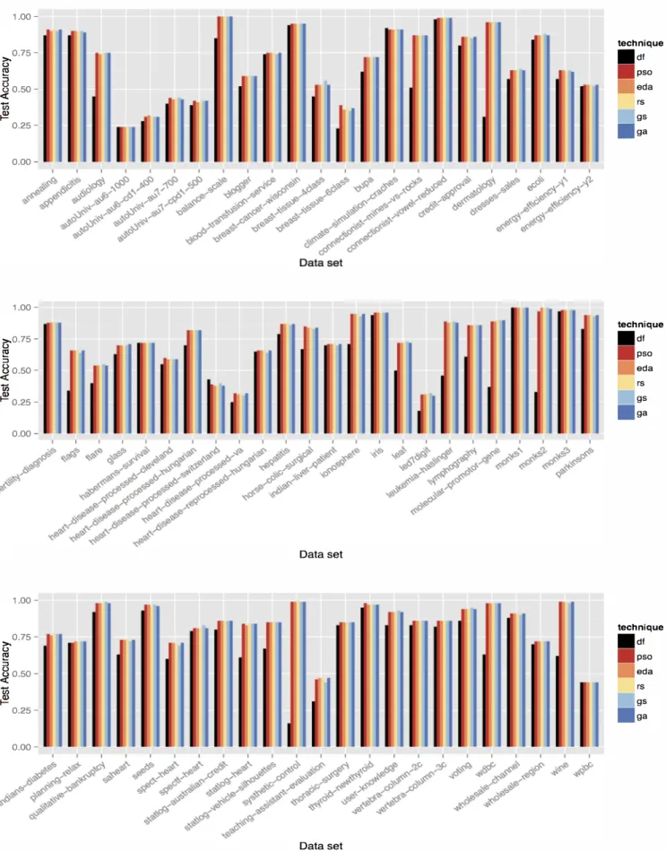
Based on the previous results, the parameter tuning tech niques were applied to each data set using the S-CV method ology. The maximum number of evaluations for each opti mization technique was fixed to 2500. Figure 4 summarizes the results for 70 data sets. The first bar shows the predictive accuracy when default values are used. Subsequent columns show the improvement in predictive performance when the tuning techniques are applied. Larger bars indicate a gain in performance. Results are averaged over 30 executions.
It should be noted that there are some cases where the tuning does not provide significant improvements. This oc cured in the data sets monks}, iris, and others originating from simple classification tasks. The data sets wpbc and
habermans-survival have shown no improvement. However, in most data sets the adjustment improves the performance of the models. The most characteristic cases are perhaps the data sets
audiology, leukemia-haslinger, statlog-heart and wine.
TABLE IV. WIN-TIE-Loss OF THE OPTIMIZATION TECHNIQUES FOR
70 DATA SETS.
Technique Win Tie Loss
GA 1 44 25 pso 3 47 20 EDA I 4 1 28 RS 2 44 24 GS 2 43 25 OF 2 4 64
These results also allow us to observe that no technique was the best on all data sets. Table IV corroborates this showing a high number of ties between the techniques. The experiments have shown that, in general, the DF values are good initial values for the SVM hyper-parameters, but in most cases tuning the hyper-parameters resulted in a substantial improvement in the accuracy of the induced models.
Additionally, we observe that a considerable number of tuning steps lead to good solutions (compared with DF) and allow RS to obtain an average accuracy similar to the MTHs. The comparison of the results obtained by GS compared to those obtained by RS allows us to observe that the latter is able to generate models that are better than the former with the same number of evaluations, a behavior already observed in the literature with other classifiers [5].
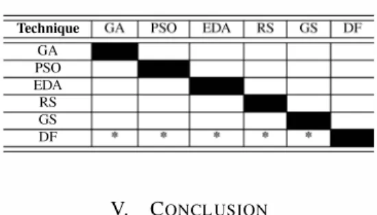
The Friedman statistical test with the Nemenyi post-hoc test and confidence level of 95% was applied for the exper imental results to compare the predictive performance of the optimization effect for all data sets. Table V presents when significant differences occurred. An asterisk means that the technique in the line is statistical different from the technique in the column with 95% confidence. According to the test, all the tuning techniques found better hyper-parameter values than the default values (DF). They also showed no difference in the predictive performance between the tuning techniques. These results support the claim that, for SVMs, a simple and faster technique such as RS is able to obtain similar results compared to more sophisticated techniques (e.g. MTH), and traditional techniques (e.g. GS). These results could be due to the low dimensional space Gust 2 hyper-parameters) and with a higher hyper-space the RS might no be so effective.
TABLE V. FRIEDMAN-NEMENYI TEST RESULT
Technique GA pso EDA RS GS OF V. CONCLUSION
This work investigated the use of the Random Search (RS) method for adjusting hyper-parameters of Support Vector Machines (SVMs). Experiments were carried out with MTHs, RS and GS over 70 data sets from VCI, mostly of low dimensionality. The experiments corroborated our hypothesis for the datasets and techniques used: RS, a simple tuning technique hyper-parameter values, can generate SVM models with predictive accuracy similar to the models generated by meta-heuristics.
RS also obtained better solutions than DF, and as good as GS. It must be observed that statistical tests showed no signif icant difference between the MTHs and the other techniques for the optimization of SVM hyper-parameters.
As future work, we intend to add pre- and post-processing hyper-parameters that may increase the complexity of the tun ing problem being addressed, and expand the experiments to include harder problems (datasets), and other ML algorithms, mainly those with a larger number of hyper-parameters. We also aim to build on, and make all our experiments available in OpenML [27], [28] for reproducibility and further study.
ACKNOWLEDGMENT
The authors would like to thank CAPES, CNPq and FAPESP (Brazilian Agencies) for the financial support.
REFERENCES
[l] P. Koch, B. Bisch!, O. Flasch, T. Bartz-Beielstein, C. Weihs, and W. Ko nen, "Tuning and evolution of support vector kernels," Evolutionary Intelligence, vol. 5, no. 3, pp. 153-170, 2012.
[2] S. Ali and K. A. Smith-Miles, "A meta-learning approach to automatic kernel selection for support vector machines," Neurocomp., vol. 70, no. 13, pp. 173-186, 2006.
[3] I. Braga, L. P. do Carmo, C. C. Benatti, and M. C. Monard, "A note on parameter selection for support vector machines," in Advances in Soft Computing and Its Applications, ser. LNCC, F. Castro, A. Gelbukh, and M. Gonzalez, Eds. Springer Berlin Heidelberg, 2013, vol. 8266, pp. 233-244.
[4] c. Soares, P. B. Brazdil, and P. Kuba, "A meta-learning method to select the kernel width in support vector regression," Machine Learning,
vol. 54, no. 3, pp. 195-209, 2004.
[5] 1. Bergstra and Y. Bengio, "Random search for hyper-parameter opti mization," 1. Mach. Learn. Res., vol. 13, pp. 281-305, Mar. 2012. [6] A. Ben-Hur and 1. Weston, in Data Mining Techniques for the Life
Sciences, ser. Methods in Molecular Biology. Humana Press, 2010, vol. 609, pp. 223-239.
[7] D. Goldberg, Genetic Algorithms in Search, Optimization and Machine Learning. Addison Wesley, 1989.
[8] 1. Kennedy, "Particle swarms: optimization based on sociocognition," in Recent Development in Biologically Inspired Computing, L. Castro and F. V. Zuben, Eds. Idea Group, 2005, pp. 235-269.
[9] M. Hauschild and M. Pelikan, "An introduction and survey of estimation of distribution algorithms," Swarm and Evolutionary Computation,
vol. 1, no. 3, pp. III - 128, 201l.
[10] c.-w. Hsu and c.-J. Lin, "A comparison of methods for multiclass support vector machines," Neural Networks, IEEE Transactions on,
vol. 13, no. 2, pp. 415-425, Mar 2002.
[11] F. Hutter, H. H. Hoos, and T. Stlitzle, "Automatic algorithm config uration based on local search," in Proceedings of the 22nd national conference on Artificial intelligence - Volume 2, ser. AAAI'07. AAAI Press, 2007, pp. 1152-1157.
[I2] N.-E. Ayat, M. Cheriet, and C. Y. Suen, "Optimization of the svm kernels using an empirical error minimization scheme," in Proceedings of the First Internat. Workshop on Pattern Recog. with SVMs.
[13] F. Friedrichs and C. Igel, "Evolutionary tuning of multiple svm param eters," Neurocomput., vol. 64, pp. 107-117, 2005.
[14] T. Eitrich and B. Lang, "Efficient optimization of support vector machine learning parameters for unbalanced datasets," Journal of Compo and Applied Mathematics, vol. 196, no. 2, pp. 425-436, 2006. [I5] O. Chapelle, Y. Vapnik, O. Bousquet, and S. Mukherjee, "Choosing
multiple parameters for support vector machines," Machine Learning,
vol. 46, no. 1-3, pp. 131-159, Mar. 2002.
[16] F. Hutter, H. Hoos, K. Ley ton-Brown, and T. Sttitzle, "Paramils: an automatic algorithm con- figuration framewor," Journal of Artificial Intelligence Research, no. 36, pp. 267-306, 2009.
[17] Y. Nannen and A. E. Eiben, "Relevance estimation and value calibration of evolutionary algorithm parameters;' in Proc. of the 20th Intern. Joint Conf. on Art. Intelligence, ser. !JCAr07, 2007, pp. 975-980. [18] C. Thornton, F. Hutter, H. H. Hoos, and K. Ley ton-Brown, "Auto
WEKA: Combined selection and hyperparameter optimization of clas sification algorithms," in Proc. of KDD-2013, 2013, pp. 847-855. [19] R. Bardenet, M. Brendel, B. Kegl, and M. Sebag, "Collaborative hyper
parameter tuning," in Proceedings of the 30th International Conference on Machine Learning (ICML-13), S. Dasgupta and D. McaUester, Eds., vol. 28, no. 2. JMLR Workshop and Conference Proceedings, 2013, pp. 199-207.
[20] J. Bergstra, D. Yamins, and D. D. Cox, "Making a science of model search: Hyperparameter optimization in hundreds of dimensions for vision architectures," in Proc. 30th Intern. Conf. on Machine Learning,
2013, pp. 1-9.
[21] S. Andradottir, "A review of random search methods," in Handbook of Simulation Optimization, ser. International Series in Operations Research & Management Science, M. C. Fu, Ed. Springer New York, 2015, vol. 216, pp. 277-292.
[22] T. A. F. Gomes, R. B. C. Prudencio, C. Soares, A. L. D. Rossi, and nd Andre C. P. L. F. De Carvalho, "Combining meta-learning and search techniques to select parameters for support vector machines,"
Neurocomput., vol. 75, no. 1, pp. 3-13, Jan. 2012.
[23] A. L. D. Rossi and A. C. P. L. F. Carvalho, "Bio-inspired optimization techniques for svm parameter tuning," in Proceed. of 10th Brazilian Symp. on Neural Net. IEEE Computer Society, 2008, pp. 435-440. [24] D. Krstajic, L. 1. Buturovic, D. E. Leahy, and S. Thomas, "Cross
validation pitfalls when selecting and assessing regression and clas sification models." Journal of cheminformatics, vol. 6, no. 1, 2014. [25] K. Bache and M. Lichman, "VCI machine learning repository," 2013.
[Online]. Available: http://archive.ics.uci.edu/ml
[26] C.-c. Chang and c.-J. Lin, UBSVM: a Library for Support Vector Machines, 2001, software available at http://www.csie.ntu.edu.tw/ cjlin/Jibsvm.
[27] 1. Vanschoren, 1. N. van Rijn, B. Bischl, and L. Torgo, "OpenML: Net worked science in machine learning," SIGKDD Explorations, vol. 15, no. 2, pp. 49-60, 2013.
[28] J. van Rijn, B. Bischl, L. Torgo, B. Gao, Y. Vmaashankar, S. Fischer,
P. Winter, B. Wiswedel, M. Berthold, and J. Vanschoren, "OpenML: A collaborative science platform," in Proceedings of ECMLPKDD 2013,