Explaining Support Vector Machines: A Color Based Nomogram.

Explaining Support Vector Machines: A Color

Based Nomogram

Vanya Van Belle1,2*, Ben Van Calster3*, Sabine Van Huffel1,2, Johan A. K. Suykens1,2, Paulo Lisboa4

1 Department of Electrical Engineering (ESAT), STADIUS Center for Dynamical Systems, Signal Processing

and Data Analytics, KU Leuven, Leuven, Belgium, 2 iMinds Medical IT, Leuven, Belgium, 3 Department of Development and Regeneration, KU Leuven, Leuven, Belgium, 4 Department of Applied Mathematics, Liverpool John Moores University, Liverpool, United Kingdom

*[email protected](VVB);[email protected](BVC)

Abstract

Problem setting

Support vector machines (SVMs) are very popular tools for classification, regression and other problems. Due to the large choice of kernels they can be applied with, a large variety of data can be analysed using these tools. Machine learning thanks its popularity to the good performance of the resulting models. However, interpreting the models is far from obvious, especially when non-linear kernels are used. Hence, the methods are used as black boxes. As a consequence, the use of SVMs is less supported in areas where interpretability is important and where people are held responsible for the decisions made by models.

Objective

In this work, we investigate whether SVMs using linear, polynomial and RBF kernels can be explained such that interpretations for model-based decisions can be provided. We further indicate when SVMs can be explained and in which situations interpretation of SVMs is (hitherto) not possible. Here, explainability is defined as the ability to produce the final deci-sion based on a sum of contributions which depend on one single or at most two input variables.

Results

Our experiments on simulated and real-life data show that explainability of an SVM

depends on the chosen parameter values (degree of polynomial kernel, width of RBF kernel and regularization constant). When several combinations of parameter values yield the same cross-validation performance, combinations with a lower polynomial degree or a larger kernel width have a higher chance of being explainable.

a11111

OPEN ACCESS

Citation: Van Belle V, Van Calster B, Van Huffel S, Suykens JAK, Lisboa P (2016) Explaining Support Vector Machines: A Color Based Nomogram. PLoS ONE 11(10): e0164568. doi:10.1371/journal. pone.0164568

Editor: Santosh Patnaik, Roswell Park Cancer Institute, UNITED STATES

Received: February 1, 2016 Accepted: September 27, 2016 Published: October 10, 2016

Copyright:©2016 Van Belle et al. This is an open access article distributed under the terms of the Creative Commons Attribution License, which permits unrestricted use, distribution, and reproduction in any medium, provided the original author and source are credited.

Data Availability Statement: All data is available within the paper and repositories listed. The first two datasets used in the paper are available from the UCI Machine Learning Repository. The Iris dataset is accessible from:http://archive.ics.uci. edu/ml/datasets/IrisThe Pima dataset from:http:// archive.ics.uci.edu/ml/datasets/Pima+Indians +Diabetes. The credit risk dataset is available from http://archive.ics.uci.edu/ml/machine-learning-databases/statlog/german/.

Funding: V. Van Belle is a postdoctoral fellow of the Research foundation Flanders (FWO). This research was supported by: Center of Excellence

Conclusions

This work summarizes SVM classifiers obtained with linear, polynomial and RBF kernels in a single plot. Linear and polynomial kernels up to the second degree are represented exactly. For other kernels an indication of the reliability of the approximation is presented. The complete methodology is available as an R package and two apps and a movie are provided to illustrate the possibilities offered by the method.

Introduction

Support vector machines (SVMs) have proven to be good classifiers in all kinds of domains, including text classification [1], handwritten digit recognition [2], face recognition [3], bioin-formatics [4], among many others. Thanks to the large variety of possible kernels, the applica-tion areas of SVMs are widespread. However, although these methods generalize well to unseen data, decisions made based on non-linear SVM predictions are difficult to explain and as such are treated as black boxes. For clinical applications, information on how the risk of dis-ease is estimated from the inputs is crucial information to decide upon the optimal treatment strategy and to inform patients. Being able to discuss this information with patients might enable patients to change their behaviour, life style or therapy compliance. Interpretation is especially important for validation of the model inferences by subject area experts. The fact that machine learning techniques are not able to find their way into clinical practice might very well be related to the lack of acquiring this information.

Offering interpretation to SVMs is a topic of research with different perspectives [5]. Identi-fication of prototypes [6] (interpretability in dual space) offers an interpretation closely related to how doctors work: based on experience from previous patients (the prototypes) a decision is made for the current patient. A second view on interpretability (interpretability in the input space) intends to offer insights in how each input variable influences the decision. Some researchers worked on a combination of both [7] and identified prototypes dividing the input space into Voronoi sections, within which a linear decision boundary is created, offering inter-pretation w.r.t. the effect of the inputs in a local way. Other approaches try to visualize the deci-sion boundary in a two-dimendeci-sional plane [8], using techniques related to self-organizing maps [9]. The current work attempts to offer a global interpretation in the input space.

The literature describes several methods to extract rules from the SVM model (see [10,11] and references therein) in order to provide some interpretation of the decisions obtained from SVM classifiers. However these rules do not always yield user-friendly results, and when inputs are present in several rules, identifying how the decision will change depending on the value of an input is not straightforward.

Several authors have therefore tried to open the black box by attempts to visualize the effect of individual inputs to the output of the SVM. In [12], Principal Component Analysis is used on the kernel matrix. Biplots are used to visualize along which principal components the class separability is the largest. To visualize which original inputs contribute the most to the classi-fier, pseudosamples with only one input differing from zero are used to mark trajectories within the plane spanned by the two principal components identified before. Those inputs with the largest trajectories along the direction of largest class separability are the most impor-tant inputs. Although this approach enables to visualize which inputs are most relevant, it is not possible to indicate how the output of the classifier (i.e. the latent variable or the estimated probability) would change in case the value of one input would change.

(CoE): PFV/10/002 (OPTEC); iMinds Medical Information Technologies; Belgian Federal Science Policy Office: IUAP P7/19/ (DYSCO, ‘Dynamical systems, control and optimization’, 2012–2017); European Research Council: ERC Advanced Grant, (339804) BIOTENSORS. This paper reflects only the authors’ views and the Union is not liable for any use that may be made of the contained information. JS acknowledges support of ERC AdG A-DATADRIVE-B, FWO G.0377.12, G.088114N. The funders had no role in study design, data collection and analysis, decision to publish, or preparation of the manuscript.

Competing Interests: The authors have declared that no competing interests exist.

A second method to visualize and interpret SVMs was proposed by [13] for support vector regression. They propose to multiply the input matrix containing the inputs of all support vec-tors with the Lagrange multipliers to get the impact of each input. This approach is again able to identify the most important inputs, but is not able to indicate how the output of the SVM changes with changing inputs.

Other work consists in visualizing the discrimination of data cohorts by means of projec-tions guided by paths through the data (tours) [14–16]. Although these methods offer addi-tional insights, they do not quantify the impact of each feature on the prediction, which is the goal of the current work.

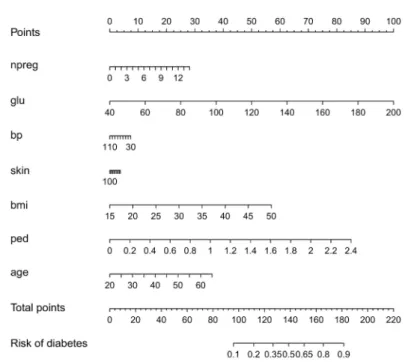
Standard statistical methods such as linear and logistic regression offer the advantage that they are interpretable in the sense that it is clear how a change in the value of one input vari-able will affect the predicted outcome. To further clarify the impact of the input varivari-ables, visualization techniques such as nomograms [17] can be used (seeFig 1). In short, a nomo-gram represents a linear model^y¼Pd_p¼1 wðpÞ_xðpÞ_{þb, withx}(p)_thepth_{input andw}(p)_the

cor-responding weight, by means of lines, the length of which is related to the range ofw(p)x(p)

observed in the training data. For each input value the contribution to the predicted outcome can instantly be read of from the plot. See Section Logistic regression models for more infor-mation. Straightforward extension of this technique to SVMs is not possible due to the fact that the SVMs are mainly used in combination with flexible kernels that can not be decom-posed into additive terms, each accounting for one single input variable. A possible extension

Fig 1. Visualization of the logistic regression model for the Pima dataset by means of a nomogram.

The contribution of each input variable x(p)_(f(p)_{= w}(p)_x(p)_{) to the linear predictor is shifted and rescaled such}

that each contribution has a minimal value of zero and the maximal value of all contributions is 100. Each input variable is represented by means of a scale and the value of the contribution can be found by drawing a vertical line from the input variable value to the points scale on top of the plot. Adding the contributions of all input variables results in the total points. These can be transformed into a risk estimate by drawing a vertical line from the total points scale to the risk scale. The importance of the inputs is represented by means of the length of the scales: variables with longer scales have a larger impact on the risk prediction.

of nomograms towards support vector machines [18] therefore focusses on the use of decom-poseble kernels [19]. The most restricting way of applying this approach is to define a kernel as the addition of subkernels that only depend on one single input. The use of a localized radial basis function kernel in [20] is only one example. The original work of [18] to represent SVMs by means of nomograms is less restrictive in the sense that kernels including interac-tions between two inputs are allowed. The idea behind these approaches is that by using a decomposible kernel, the latent variable of the SVM can be expressed as a sum of terms, depending on one input. As such, the SVM becomes a generalized additive model and can be visualized by means of a nomogram. In [18] non-linearities are visualized by drawing two-dimensional curves instead of straight lines in the nomogram, such that non-linearities can more easily be represented than when using a line. They also allow for interactions between two inputs, but, as with standard nomograms, they can only be represented after categoriza-tion of one of the two involved inputs.

In contrast with the approaches found in the literature, this work does not intend to adapt the kernel nor the SVM model formulation. This work takes the first steps in answering the question whether existing SVMs in combination with generally used kernels can be explained and visualized, in which circumstances this is possible and to which extent. Instead of adapting the kernel, the nomogram representation is altered to easily allow for non-linear and two-way interaction effects. This is achieved by replacing the lines by color bars with colors offering the same interpretation as the length of the lines in nomograms. It is indicated for which kernels and kernel parameters the representation by means of this color based nomogram is exact. In cases where the visualization is only approximate, additional graphs indicate why the approxi-mation is not sufficient and how this might be solved. The current approach is related to the work in [21,22], where a Taylor expansion of the RBF kernel is used to extract interpretable and visualizable components from an SVM with RBF kernel. In this work, the expansion is indicated for linear, polynomial and RBF kernels. Additionally, the expansion is used to visual-ize the working of an existing SVM, whereas in the previous work a new model was created after feature selection by means of iterativel1regularization of a parametric model with the

dif-ferent components as inputs.

The remainder of this work is structured as follows. First, a short introduction to SVM clas-sification is given. It is shown how a nomogram is built for logistic regression models and how an alternative color based nomogram for logistic regression was used in [23]. Next, it is

explained how to reformulate the SVM classifier in the same framework. Experiments on artifi-cial data illustrates the approach and indicates possible problems and solutions. Finally, real life datasets are used to illustrate the applicability on real examples. The work concludes with information on the available software and a discussion on the strengths and weaknesses of the study.

Methods

This section clarifies how an SVM can be explained by means of a color based nomogram. For generality, we start with a brief summary of an SVM classifier, followed by an introduction on the use of a nomogram to visualize logistic regression models.

In the remainder of this work,xiðpÞ m

will indicate themthpower of thepthinput variable of theithobservationxi.

SVM classifier

Suppose a datasetD¼ fxi;yig N

i¼1is a set ofNobservations with input variablesxi 2R d

and class labelsyi2{−1, 1}. The SVM classifier as defined by Vapnik [24] is formulated as

min w;b; 1 2w T_wþCX N i¼1 _i subject to y_i wT_φðx iÞ þb ð Þ 1 _i; 8 i¼1;. . .;N _i 0; 8 i¼1;. . .;N: 8 < : ð1Þ

To facilitate the classification, a feature mapφ() is used to transform the inputs into a higher dimensional feature space. The coefficients in this higher dimensional feature space are denoted byw2Rn_φ

. The trade-off between a smooth decision boundary and correct classifica-tion of the training data is made by means of the strictly positive regularizaclassifica-tion constantC.

The dual formulation of the problem stated inEq (1)is found by defining the Lagrangian and characterizing the saddle point and results in:

min a 1 2 XN i;j¼1 yiyjφðxiÞ T φðxjÞaiaj XN i¼1 a_i subject to XN i¼1 a_iyi ¼0 0a_i C; 8 i¼1;. . .;N: 8 > > > < > > > : ð2Þ

The power of SVMs lies in the fact that the feature map does not need to be defined explic-itly. An appropriate choice of a kernel functionK(x,z) for any two pointsxandzthat can be expressed as

Kðx;zÞ ¼φðxÞTφðzÞ;

makes it possible to use an implicit feature map.

A class label for a new pointxcan then be predicted as ^ y¼ sign X N i¼1 a_iyiKðxi;xÞ þb ! :

Here‘¼PN_i¼1a_iyiKðxi;xÞ þbis called the latent variable. In order to obtain probabilities, the sign() function can be replaced by a functionh(). In this work the latent variable will be converted into a risk estimate by using it as a single input in a logistic regression model with two parameters. This approach is known as Platt’s rule [25,26].

Visualization of risk prediction models

Logistic regression models. In statistics, regression models can be visualized using nomo-grams [17]. More recently color plots have been proposed [23] to represent contributions to the linear predictor (herePd_p¼1w

ðpÞ_xðpÞ_{þb) depending on only one or by extension maximally} two input variables. The nomogram for logistic regression (LR) builds on the fact that the model in its most basic form can be written as

^ p¼h X d p¼1 wðpÞ_xðpÞ_þb ! ; ð3Þ

whereh() is a link function (here the sigmoid function) transforming the linear predictor to a chance,w(p)is the coefficient corresponding to thepthinput variablex(p)andbis a constant. The contribution of each input variablex(p)to the linear predictor can thus be visualized by

plottingf(p)(x(p)) =w(p)x(p). In fact, for nomograms these terms are rescaled to start from 0 to a maximum of 100 points. Doing so makes clear that the range of the contributions is important. A wide range of the contributions for one input variable indicates that changing the value of this input, can have a large impact on the linear predictor and as such on the risk estimate.

Fig 1clarifies this approach for a logistic regression model trained on the Pima Indian diabetes dataset from the UCI repository [27]. The training data as provided in the R packageMASS

[28,29] was used to train the logistic regression model. The nomogram was generated using thermspackage [28,30]. To obtain the risk estimate for an observation, the points corre-sponding to each input variable are obtained by drawing a vertical line from this value up to the points scale on top of the plot. These points are added to obtain the total points, which are converted to a risk by means of the bottom two scales.

A similar approach using the methods proposed in [23] is illustrated inFig 2. Instead of scales, color bars are used, the color of which indicates the contribution of the input variable value. In this case, the contributions are shifted to make sure that the minimal contribution of each input is zero. The contributions are not rescaled. The importance of the inputs is clear from the color. The intenser the red color becomes within the color bar, the more impact this input has (similar to the length of the scales in the nomogram). To obtain a risk estimate for an observation, the procedure is as follows. For each input, find the color corresponding to the input’s value. This color is converted to a point by means of the color legend at the right.

Fig 2. Visualization of the logistic regression model for the Pima dataset by means of a color plot or color based nomogram. The contribution of each input variable x(p)(f(p)= w(p)x(p)) to the linear predictor is shifted such that each contribution has a minimal value of zero. To obtain a risk estimate for an observation, the color corresponding to the input’s value needs to be indicated. This color is converted to a point by means of the color legend at the right. Repeating this for each input and summing the resulting points, yields the score. This score is then converted into the risk estimate by means of the bottom most color bar. The importance of the inputs is represented by means of the redness of the color: variables with a higher intensity in red have a larger impact on the risk prediction.

Repeating this for each input and summing the resulting points, yields the score. This score is then converted into the risk estimate by means of the bottom most color bar. A more detailed explanation of how this color based nomogram is constructed from the risk prediction model is given inS1 Text.

From both approaches (nomogram and color-based plot) it is easily concluded that glucose, the pedigree function and bmi are the most influential inputs.

Support vector classifiers. Whether or not an SVM classifier can be interpreted in the same way as explained above and represented by similar graphs, depends on the choice of the kernel. A derivation for the linear, polynomial and RBF kernel is given here.

When using a linear kernelKlinðx;zÞ ¼

P_d p¼1x

ðpÞ_zðpÞ_{, the extension of the nomogram to an} SVM is easily made. The predicted risk is found as:

^ y¼h X N i¼1 a_iyiKðxi;xÞ þb ! ¼h X N i¼1 a_iyi Xd p¼1 xðpÞi xðpÞþb ! ;

such that the contribution of thepthinput variable to the linear predictor is defined as

fðpÞ _¼X N i¼1 a_iyix ðpÞ i xðpÞ:

This expansion enables to visualize an SVM model with a linear kernel using plots of the type presented inFig 2. Each contributionf(p)is then represented by a color bar. The points that are allocated to the value of an input are read off by means of the color legend. The score is obtained by addition of all points. The functionh() converting this score to a risk estimate is visualized by another color bar at the bottom of the graph. Examples of this type of representa-tion for SVM models are given in Secrepresenta-tion Results.

This approach can also be extended to other additive kernels [31] and ANOVA kernels [19,

24], in which kernels are expressed as a sum of subkernels, each of which depend on a restricted set of input variables. In cases were no more than two inputs are involved in each subkernel, the representation will be exact. Visualization of two-way interaction effects is done by the use of color plots instead of color bars. Examples of this approach are given in Section Results.

For the polynomial kernelKpoly(x,z) = (axTz+c)δ, withδa positive integer, an expansion

of the latent variable is found by use of the multinomial theorem [32]

ðxð1Þ þ þxðdÞ_Þd ¼ X k1þþkd¼d d k1;. . .;kd ! Y 1pd xðpÞkp : ð4Þ

The latent variable of the SVM classifier can then be written as: ‘ ¼X N i¼1 a_iyiKpolyðxi;xÞ þb ¼X N i¼1 a_iyiðaxTixþcÞ d þb¼X N i¼1 a_iyi a Xd p¼1 xiðpÞxðpÞþc !d þb ¼X N i¼1 a_iyi c d_þadX d p¼1 xðpÞi d xðpÞd_þX d p¼1 X kpþkc¼d d kp;kc 0 @ 1 A_ak_pxðpÞ i kpxðpÞkpckcþ 2 4 Xd p¼1 X q6¼p X kpþkq¼d kp;kq6¼d d kp;kq 0 @ 1 A _axðpÞ i xðpÞ k_p axðqÞi xðqÞ k_q þ Xd p¼1 X q6¼p X kpþkqþkc ¼d kp;kq;kc6¼d kpþkq6¼d kpþkc 6¼d k_qþk_c 6¼d d kp;kq;kc 0 @ 1 A _axðpÞ i xðpÞ kp axðqÞi xðqÞ kq ckc_þD 3 7 7 7 7 7 7 7 7 7 7 7 7 7 7 7 7 7 7 7 7 7 7 7 7 7 7 7 7 7 7 5 þb ¼X N i¼1 a_iyi b 0_þX d p¼1 gðpÞ _xðpÞ i ;xðpÞ þX d p¼1 X q6¼p gðp;qÞ _xðp;qÞ i ;xðp;qÞ þD ! þb ¼X d p¼1 fðpÞ _xðpÞ i ;xðpÞ þX d p¼1 X q6¼p fðp;qÞ _xðp;qÞ i ;xðp ;qÞ þb@_þD‘

Here, we definef(p) as the functional form of thepthinputx(p), i.e. the contribution to the latent variable that is solely attributed tox(p). In analogy,f(p,q)is defined as the contribution to the latent variable that is attributed to the combination of inputsx(p)andx(q). The derivation above, shows that for eacha,candδ, an SVM classifier with a polynomial kernel can be expanded in main contributionsf(p), contributionsf(p,q)involving two input variables and a rest termΔℓ, including all contributions involving a combination of more than two input vari-ables. From the equations, it can be seen that wheneverdorδare not higher than 2, the expan-sion of the polynomial kernel is exact, i.e.Δℓ= 0.S2 Textindicates how the termsf(p)andf(p,q)

When using the popular Radial Basis Function (RBF) kernel, the extension is based on a similar approach. The RBF kernel is defined as

KRBFðx;zÞ ¼ exp 1 s2jjx zjj 2 2 ¼ exp gjjx zjj22 ; withs2 _¼1

gthe kernel width. Using the Taylor expansion of the exponential function, this ker-nel can be written as

KRBFðx;zÞ ¼ X1 n¼0 ð 1Þngn_{ðjjx zjj}2 2Þ n n! :

Application of the multinomial theorem results in

KRBFðx;zÞ ¼ X1 n¼0 ð 1Þngn n! X k1þþkd¼n n k1;. . .;kd ! Y 1pd xðpÞ _zðpÞ2 kp : ð5Þ

The question whether SVM classifiers using the RBF kernel can be visualized and explained as in Figs1and2is now reduced to the question whether we can writeEq (5)as the addition of terms only depending on one input variable, or by extension also including terms depending on two input variables. To achieve this,Eq (5)is written as:

KRBFðx;zÞ ¼ X1 n¼0 ð 1Þngn n! Xd p¼1 ðxðpÞ _zðpÞ_Þ2n " þX d p¼1 X q6¼p X kpþkq¼n kp;kq6¼n n kp;kq ! ðxðpÞ _zðpÞ_Þ2kp_ðxðqÞ _zðqÞ_Þ2kq 3 7 7 7 7 7 7 7 5 þD;ð6Þ ¼X d p¼1 gðpÞ _xðpÞ_;zðpÞ_þX d p¼1 X q6¼p gðp;qÞ _xðp;qÞ_;zðp;qÞ_{þD: ð7Þ}

The latent variable can then be written as:

‘¼X N i¼1 a_iyiKRBFðxi;xÞ þb ð8Þ ¼X N i¼1 a_iyi Xd p¼1 gðpÞ _xðpÞ i ;xðpÞ þX d p¼1 X q6¼p gðp;qÞ _xðp;qÞ i ;xðp ;qÞ þD " # þb ð9Þ ¼ Xd p¼1 fðpÞ _xðpÞ i ;xðpÞ þ Xd p¼1 X q6¼p fðp;qÞ _xðp;qÞ i ;xðp ;qÞ þb00 þD‘ : ð10Þ

The kernel function can thus be written as a part dependent on single inputs, i.e. the first term in the above equation, a part depending on two inputs, i.e. the second term, and a rest part, including terms depending on a combination of more than two inputs. A formal defini-tion of these terms is given inS2 Text. The only question that remains is whether the rest term

is small enough to be ignored without preformance reduction. The experiments in the next Sec-tion illustrate whether and when this is the case. WheneverΔℓcan be ignored, the SVM model can be visualized by use of color based nomograms, representingf(p)by color bars,f(p,q)by color plots and converting the latent variable (visualized via the score) into a risk estimate by means of another color bar. A more detailed explanation of how the color based nomogram is constructed from the above expansion is presented inS1 Text.

Results

In this Section, it is investigated whether it is possible to approximate the SVM model by an additive model, only including terms that can be visualized. Stated otherwise, the SVM model will be approximated using the expansions obtained in the previous sections and ignoring the rest termΔℓ. This approach is illustrated on several simulated and real-life datasets. Since the proposed visualization method is exact for two-dimensional problems, only problems with at least three input variables will be discussed here. The first examples are based on artificial data-sets with only 3 input variables, of which only two are relevant. Each artificial dataset contains 1000 observations, 500 of which are used for training, the remainder for testing the SVM model. It is assumed that, since only two inputs are necessary for the true classification, the approximation method should be able to explain the resulting SVM models: if one input is irrelevant, then why would a well performing SVM model use contributions that involve this input variable? The artificial problem settings are illustrated inS3 Text, where the class separa-tion is illustrated in the two relevant dimensions. We conclude with an applicasepara-tion on three real-life datasets from the UCI depository [27] (Fisher Iris, Pima Indians diabetes and German credit risk data).

When using SVMs in combination with an RBF or polynomial kernel, multiple parameters need to be set: (i) the regularization constantC, (ii) the width1

gof the RBF kernel or the degree δof the polynomial kernel. For simplicity, we keep both the scaleaand the biascof the polyno-mial kernel equal to 1. A grid search in combination with 10-fold cross validation is used to select the optimal parameter set on the training set.

In all the examples we use a fixed grid to tune the parameters. The regularization constantC

is varied over [10−7, 102], using ten steps (exponential grid). The inverse kernel widthγis var-ied over [2−7, 22], using ten steps (exponential grid). The degree of the polynomial kernel can range from 1 to 4. Class probabilities are obtained by means of a sigmoid function, the parame-ters of which are fitted using 3-fold cross-validation on the training data (the default in the R packagekernlab). Parameter tuning is performed using the R packagecaret[33]. The R packagekernlab[34] is used to train the SVMs.

Regarding the visualizations, it is opted to show the plots with contributions that are shifted such that the median of all contributions is zero. A diverging colormap is used such that a value of zero corresponds to a white color, negative values are represented in blue and positive values in red. The most important input variables are those with the largest color range.

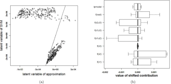
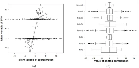
Before continuing to the experiments, it is stressed that visualizing an SVM model based on the proposed approximation and extracting how the SVM model works based on this approxi-mation is only possible after confirapproxi-mation that the approxiapproxi-mation is valid: the rest term should be small. Otherwise, conclusions drawn from the approximation cannot be assumed to be cor-rect. In order to check the validity of the approximation, two types of plots are provided. A first plot relates the latent variable of the SVM model with the approximated latent variable (i.e. the latent variable of the SVM model without the rest termΔℓ). An example of this type of plot is given inFig 3(a). The straight line in the plot indicates where the points should be located when the approximation is valid. A second plot represents the ranges of all contributions in the

expansion of the latent variable. The range of the latent variable of the SVM model (indicated by lpmodel) is given as well. Whenever the approximation is valid, the rest term will be small in comparison with the latent variable. An example of this plot is given inFig 3(b).

Artificial examples

Two circles problem. Consider a dataset with three input variables, only two of which are relevant. The observations are all elements of one of two classes. All elements of one class are located on a circle and both circles are concentric. SeeS3 Textfor a visualization of this setting. The SVM classifier with the highest cross-validation performance using an RBF kernel has parameter valuesγ= 2 andC= 10−5. The resulting classifier is able to classify the training sam-ples perfectly, i.e. an accuracy of 100%. The same accuracy is obtained for the test set.

To check whether the proposed method is able to explain the SVM classifier, the latent vari-ables of the SVM model and the approximation are plotted against each other inFig 3(a). Only 41% of the training datapoints get the same class label by the approximation and the SVM model. To explain this malfunctioning, the individual terms in the approximation and the rest term are reported inFig 3(b). The range of the latent variable of the SVM model (indicated as lpmodel) is added as a reference. Since the range of the rest term is large in comparison with the other terms, the rest term can not be ignored. As a result, the approximation method pro-posed here will not be able to explain the SVM model.

This experiment raises the question how the SVM achieves a good performance despite tak-ing non-relevant information (i.e. higher-order terms includtak-ing input variables of which it is known that they are irrelevant) into account. To answer this question, the correlation between the rest term and the different terms in the approximation are studied (results not shown). The rest term is highly correlated with the interaction betweenx(1)andx(2)(Pearson correlation coefficient = -0.993). The rest term can thus be explained as an interaction between the first

Fig 3. Performance of the approximation method (i.e. the expansion without the rest termΔℓ) on the two circles data. (a) Latent variables of the SVM model with RBF kernel and the approximation. The

approximation is not able to approximate the latent variables of the SVM model. (b) Contributions of the approximation of the SVM model and the rest term. The box-plots visualize the range of the different contributions. The upper boxplot indicates the range of the latent variable of the SVM model. In this example the range of the rest term cannot be ignored in comparison with the ranges of the other contributions. As such, the approximation of this specific SVM model cannot serve as an explanation of the SVM model. doi:10.1371/journal.pone.0164568.g003

two input variables and not as a higher order interaction effect as was expected. As such, drop-ping the rest term in the approximation results in loss of information.

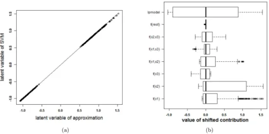
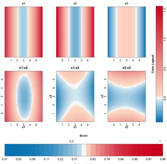
To investigate whether the above problem is due to the SVM model or due to the expansion in individual terms, other SVM models, with other tuning parameters but similar cross-valida-tion results, are analysed. The same 10-fold cross validacross-valida-tion performance can be achieved from a variety of parameter values. As such, the approximation method is applied a second time. This time, a cross-validation performance of at least 95% of the optimal performance is required and the kernel width should be as large a possible. The validity of the approximation of this second SVM model, with parameter valuesγ= 2−7andC= 10, is analysed inFig 4. The approximation is very good and the rest term can be ignored. As such, the proposed approxi-mation is able to explain the SVM classifier. The visualization of this model (seeFig 5) reveals that the contributions ofx(1),x(2)and their interaction are most important. This SVM classifier and the approximation obtain a performance accuracy of 100% on training and test set.

To compare the working of different kernels, the polynomial kernel is used on the same example. The best performing kernel had a degreeδ= 2 and the regularization constant was

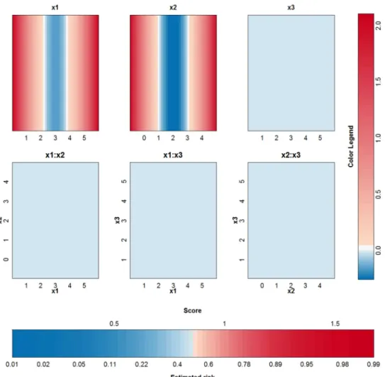
C= 0.01. The approximation is able to perfectly explain the SVM model since the degree of the kernel is not larger than 2. The SVM model is approximated by the terms visualized inFig 6. Comparison withFig 5instantly shows that a polynomial kernel is better suited for the job: the value of the irrelevant inputx(3)is not used by the polynomial kernel. Only the main effects of the first two input variables are necessary to obtain a classifier with 100% accuracy.

To compare the proposed color based nomogram with existing tools for logistic regression, a logistic regression model allowing polynomial transformations of the input variables is trained using thelrmfunction within thermspackage in R [30]. The model includes polyno-mial transformations of all input variables of the first and second degree. The resulting

Fig 4. Performance of the approximation method (i.e. the expansion without the rest termΔℓ) on the two circles data (second SVM model). (a) Latent variables of the SVM model with RBF kernel and the

approximation. The approximated latent variable is a good estimate of the latent variable of the SVM model. (b) Contributions of the approximation of the second SVM model and the rest term. The box-plots visualize the range of the different contributions. The upper boxplot indicates the range of the latent variable of the SVM model. In this example the range of the rest term can be ignored in comparison with the ranges of the other contributions. As such, the approximation of this specific SVM model will be able to explain the classifier.

nomogram is represented inFig 7. The model results in an accuracy of 100% on training and test set. The non-linear relationship is visualized by repetition of the input axis.

Swiss roll problem. As a second example, an SVM model is trained on the artificial two-class swiss roll example. The data are points in a three-dimensional space and non-linearly sep-arable in a 2-dimensional plane spanned byx(1)andx(2). The third variable is again irrelevant. SeeS3 Textfor an illustration of this setting.

The tuning parameters resulting in the largest 10-fold CV performance for the SVM model with RBF kernel areγ= 4 andC= 10. The latent variable of the SVM model and the approxi-mation as well as the ranges of the contributions, the rest term and the latent variable of the SVM model are shown inFig 8. One can clearly see that the approximation is not able to explain the SVM classifier. The rest term cannot be ignored in this case.

In contrast with the previous artificial example, looking for another optimal parameter pair does not yield a satisfying solution. This can be explained by the fact that the swiss roll example is highly non-linear and a small kernel width is necessary to obtain a good performance. To have a small rest term, a large kernel width is necessary, to reduce the influence of higher-order interaction terms. Scatterplots between all contributions and the rest term (plot not shown) explain why dropping the rest term has such a dramatical effect: the rest term is highly (inversely) correlated with the contribution of the interaction betweenx(1)andx(2)(Pearson

Fig 5. Visualization of the second SVM model with RBF kernel on the example of the two circles.

correlation coefficient = -0.968). Investigation of the Pearson correlations between the terms of the approximation reveals that the contribution of the interaction betweenx(1)andx(3)is highly (inversely) correlated with the contribution ofx(1)(Pearson correlation coefficient = -0.965) and the contribution of the interaction betweenx(2)andx(3)is highly (inversely) corre-lated with the contribution ofx(2)(Pearson correlation coefficient = -0.962). The rest term in

Fig 6. Visualization of the third SVM model (polynomial kernel) on the example of the two circles.

doi:10.1371/journal.pone.0164568.g006

Fig 7. Nomogram of a logistic regression model including polynomial transformations of the input variables for the two circles problem. The non-linearities are visualized by the use of two axes for each

input.

this example is seemingly used to counter-balance other contributions. The same is true for the interaction terms involvingx(3). All these findings indicate that the third input variable might be dropped before building the SVM. Results of this approach are not shown here since this yields a two-dimensional problem for which the approximation is exact.

Note that for the example on the two circles, selection of the most relevant input variables is an alternative (and probably preferred) to the solution proposed in the previous Section.

Checkerboard problem. This last artificial example illustrates that in some cases it is pos-sible to explain an SVM model using one kernel type, while it is not pospos-sible to explain an SVM model trained on the same data using another kernel type. To illustrate this, a checkerboard problem with 9 blocks in the plane spanned byx(1)andx(2)is used. A third input variable is again irrelevant. A visualization of this setting is provided inS3 Text. The two SVM models with optimal tuning parameters are: a first SVM model with an RBF kernel (γ= 2−4and

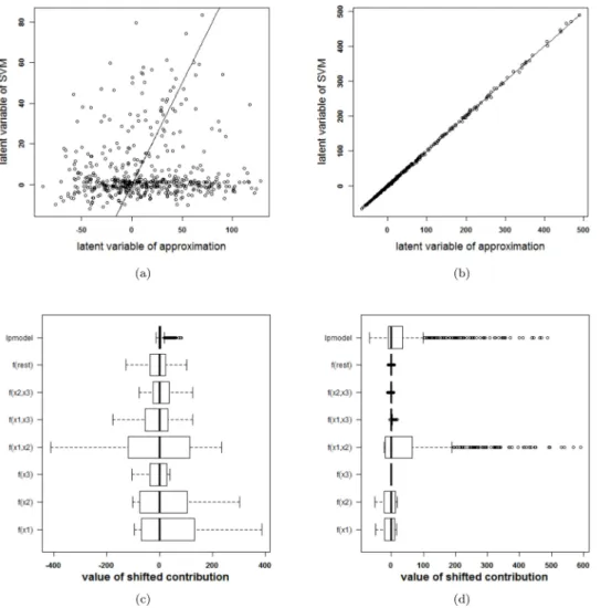
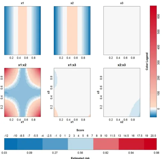
C= 105) and a second SVM model with a polynomial kernel (δ= 4 andC= 100). For both models, the optimal tuning parameters by means of 10-fold cross validation are used. The latent variables and the terms in the approximations for both models are given inFig 9. The accuracy of the SVM with RBF kernel on the training data is 0.96% and on the test data 0.91%. The accuracy of the SVM with polynomial kernel on the training data is 0.99% and on the test data 0.96%. The SVM model with an RBF kernel and its approximation agree on the class label in only 56% of the observations in the training data. The use of another parameter pair does not yield a better approximation. For the polynomial kernel, the agreement is 99%. This perfor-mance difference of the approximation method is also seen inFig 9, where a very large rest term is noted for the expansion of the SVM with RBF kernel and a very small rest term is seen when using the polynomial kernel.Fig 10illustrates the visualization of the SVM model with the polynomial kernel. This visualization is very valuable since it clearly indicates that the third variable is not necessary and the estimated functional forms of the other effects are correct.

Overlapping Gaussians. In this last artificial problem a classification problem of two strongly overlapping classes is used. The data of these two overlapping Gaussians are illustrated

Fig 8. Performance of the approximation method (i.e. the expansion without the rest termΔℓ) on the swiss roll problem. (a) Latent variables of the SVM model with RBF kernel and the approximation. The

approximation is not able to approximate the latent variables of the SVM model. (b) Contributions of the approximation of the SVM model and the rest term. The box-plots visualize the range of the different contributions. The upper boxplot indicates the range of the latent variable of the SVM model. In this example the range of the rest term cannot be ignored in comparison with the ranges of the other contributions. As such, the approximation of this specific SVM model cannot serve as an explanation of the SVM model. doi:10.1371/journal.pone.0164568.g008

inS3 Text. For an SVM model using an RBF kernel the optimal tuning parameters by means of 10-fold cross validation areγ= 2−6andC= 100. The latent variables and the terms in the approximations for both models are given inFig 11. Since the rest term is very small, the approximation can be used to explain the SVM model. The accuracy of the SVM with RBF ker-nel on the training data is 78% and on the test data 75%. The accuracy of the approximation on the training data is 78% and on the test data 74%. The SVM and the approximation agree on 100% of the cases in the training set and on 99.8% of the cases in the test set.Fig 12illustrates the visualization of the SVM model.

Real life data

The IRIS dataset. The proposed approach is applied to the IRIS dataset [27,35] and using an RBF kernel. This data contains information on 150 cases, four input variables and a class

Fig 9. Comparison of the performance of the approximations (i.e. the expansion without the rest termΔℓ) of two SVM models on the checkerboard problem. (a)-(c): RBF kernel, (b)-(d): polynomial

kernel. (a)-(b): Latent variable of the approximation versus latent variable of the original SVM model. (c)-(d): Range of all contributions in the approximation, the rest term and the latent variable of the SVM model. For the RBF kernel, the rest term is much larger than the latent variable, resulting in an approximation that is unable to explain the SVM model. For the polynomial kernel, the rest term is negligible in comparison with the other terms and the approximation is nearly perfect.

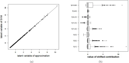
label. The labels are setosa, versicolor and virginica. For the purpose of this work, the output label was defined as species of type versicolor. An SVM was trained on 100 randomly chosen observations and tested on the remaining 50. The classifier obtained from parameter values that achieve the highest 10-fold cross validation performance (γ= 2−5andC= 100) is repre-sented inFig 13. The SVM achieves an accuracy of 99% and 96% on training and test set respectively. The approximation achieves an accuracy of 98% and 96% on training and test set respectively. The validity of the approximation is illustrated inFig 14. Since the rest term is very small, the approximation yields latent variables that are very close to the latent variables obtained by the original SVM model. The approximation performs very good in this case and agrees on class labels with the SVM model in 98% of the training cases and in 100% of the test cases. From the visualization of the model it is seen that sepal length (SL), petal length (PL) and petal width (PW), and the interaction between PL and PW contribute the most to the latent variable (colors range to the extremes of the color legend). This is also confirmed by investigat-ing the ranges of the contributions (see SectionDiscussionfor a discussion on the importance of the latter.) A bivariate plot (seeS1 Fig) indicates that PL and PW are most important for class separation in a linear setting. The interaction between PL and PW is also valuable.

Fig 10. Visualization of the SVM model with polynomial kernel on the checkerboard example. It can

be seen that all contributions involving x(3)do not contribute in a large extent since the range of these contributions is very small in comparison with the other contributions.

The Pima Indians data set. The Pima Indians dataset [27,29] contains 532 cases with complete information for women who were at least 21 years old, of Pima Indian heritage and living near Phoenix, Arizona. Seven different input variables were available: number of preg-nancies (npreg), plasma glucose concentration (glu), diastolic blood pressure (bp), triceps skin fold thickness (skin), body mass index (bmi), diabetes pedigree function (ped) and age. The outcome is whether or not these women have diabetes according to World Health Organiza-tion criteria. The SVM model with RBF kernel was trained on a random set of 200 of these women, as provided as a training set in the R packageMASS[29]. The classifier obtained from parameter values that achieve the highest 10-fold cross validation accuracy (γ= 2−7andC= 1) is represented inFig 15. The accuracy of the approximation is illustrated inFig 16. Since the rest term is very small, the approximation yields latent variables that are very close to the latent variables obtained by the original SVM model. The approximation performs very good in this case and agrees on the estimated class labels with the SVM model in 100% of the cases. The SVM achieves an accuracy of 78% on training and test set. The approximation also achieves an accuracy of 78% on training and test set. From the visualization of the model it is seen that the interaction effects are of minor importance (very light colors for all ranges of the input vari-ables). The main effects of blood pressure and skin thickness are less important than the other main effects. Comparing this result with feature selection methods in the literature confirms these results. In [21] 12 feature selection methods from the literature are compared on the Pima dataset. The blood pressure and the skin thickness are selected three times among these 12 methods, whereas all other variables are selected at least four times. In [36] different feature selection methods are also compared on the Pima dataset. Ranking features according to their importance (see Table 3 in [36]) also indicates that the blood pressure and the skin thickness are least important.)

German credit risk data. An SVM with a polynomial kernel is used to illustrate the approach on the German credit risk data [27]. The data is taken fromhttps://onlinecourses. science.psu.edu/stat857/node/215, and a random subset of 500 observations is used to train the

Fig 11. Performance of the approximation method (i.e. the expansion without the rest termΔℓ) on the two Gaussians data. (a) Latent variables of the SVM model with RBF kernel and the approximation. The

approximated latent variable is a good estimate of the latent variable of the SVM model. (b) Contributions of the approximation of the SVM model and the rest term. The box-plots visualize the range of the different contributions. The upper boxplot indicates the range of the latent variable of the SVM model. In this example the range of the rest term can be ignored in comparison with the ranges of the other contributions. As such, the approximation of this specific SVM model will be able to explain the classifier.

SVM, the remaining 500 observations are used to test the SVM. In this example only 6 inputs are selected to predict the creditability of the applicants: the status of applicant’s account in the bank (balance, categorical input), the duration of the credit in months (cr.dur.), the purpose of the credit (purpose), the amount of credit asked for (amount), the duration of the applicant’s present employment (employ.dur.), and the applicant’s duration of residence (address.dur.). The classifier obtained from parameter values that achieve the highest 10-fold cross validation accuracy (δ= 2 andC= 1) is represented inFig 17. Since the degree of the polynomial kernel equals 2, the visualization is an exact representation of the SVM model. The accuracy on the training and test set are 75% and 76% respectively. Looking at the interaction effects, it is clear that most of the interactions are not relevant (white color in the graph). Taking the range of the contributions into account (seeFig 18) illustrates that the most important effects are the effects of balance, credit duration, amount of the credit and interactions between these. A sec-ond SVM is built using only these 3 inputs, resulting in a polynomial kernel of the third degree and a regularization constantC= 0.01. The model is visualized inFig 19and the correctness of the representation is illustrated inFig 20. It is clear that the approximation yields latent vari-ables that are in line with those obtained from the SVM classifier. The accuracy of the model and approximation on the training set is 73%, for the test set this accuracy is 76%. The approxi-mation and the SVM model agree on the predicted class label in 99% of the cases.

Fig 12. Visualization of the SVM model with RBF kernel on the example of the two Gaussians.

What can we learn from this representation? It has to be noted that all effects containing the same input should be considered together when interpreting the results. With more than 2 inputs, this is however impossible, so the effects should be interpreted considering all other inputs constant. For interaction effects the interpretation is harder since one input can occur in more than one interaction effect. For this example it is noted that having a higher balance on the current account increases the chance of being creditable. A longer duration of the credit decreases this chance. The same effect is noted for an increasing credit amount. Looking at the interaction effect of balance and credit duration, it is noted that for a duration larger than 20– 25 months, the main effect of the balance on the account is amplified, whereas for a short credit duration the effect of balance is opposite to the main effect. For a low balance on the current account, an increasing credit amount increases the chance of being creditable. This seems counterintuitive, however this increase (increase in points indicated by the color legend) is lower than the decrease indicated in the main effect of the credit amount. As such, the interac-tion is making a small correcinterac-tion w.r.t. the main effect, depending on the balance. From the interaction effect between credit amount and credit duration it could be concluded that a higher credit duration and amount increases the chance of being creditable. However, this interpretation leaves out the main effects of the involved inputs. To aid in this complex inter-pretation, the contributions of all effects are plotted (Fig 21) for three applicants: applicant 1

Fig 13. Visualization of the SVM model on the IRIS data set.

(balance = 4, credit duration = 35, credit amount = 10000), applicant 2 (balance = 4, credit duration = 35, credit amount = 15000), applicant 3 (balance = 4, credit duration = 50, credit amount = 10000). This type of summary for one observation was proposed in [23] and is related to the work in [37,38]. The displayed charts illustrate how the chances on creditability are obtained from the different input values. Comparison of the charts for different applicants illustrates the change in effects of the inputs. Comparing applicant 1 and 2 reveals that the increase in amount implies a decrease in the contribution of amount by 3.57 points, the effect of the interaction between balance and amount increases by 0.8 points and the effect of the interaction between amount and credit duration increases by 0.87 points. The result is a reduc-tion of the creditability of the applicant. Comparing applicant 1 and 3 indicates that an increase in the credit duration yields a reduction of 0.84 points for the main effect of credit duration, an increase of 0.73 points due to the interaction of credit duration and balance, and an increase of 0.89 points due to the interaction of credit duration and amount. As such, an increase of the credit duration would increase the chance of being creditable.

To compare the proposed color based nomogram with the standard nomogram when deal-ing with non-linearities and interactions, a nomogram was created for a logistic regression model including only linear main and interaction effects for the reduced set of input variables. Thelrmfunction within thermspackage in R [30] was used for this purpose. The resulting nomogram is represented inFig 22. To create this nomogram, it was necessary to categorize continuous input variables (i.e cr.dur. and amount). To make the graph readable, only 3 cate-gories for amount were used. For all inputs involved in an interaction, combinations of input variables are made such that for each input only one point needs to be read from the graph. Since all inputs interact with each other in this example, only one point needs to be read from the graph. An obvious disadvantage of this representation, is the loss of information due to the categorization of continuous inputs. Additionally, it was impossible to represent a full model in a one page graph, since the number of possible combinations becomes too large. Getting a global view on the risk prediction process from this representation is less straightforward as

Fig 14. Performance of the approximation method (i.e. the expansion without the rest termΔℓ) on the IRIS data. (a) Boxplots of the contributions of the approximation of the SVM model, the rest term and the

latent variable of the SVM model. The range of the rest term can be ignored in comparison with the ranges of the other contributions. (b) Latent variable of the original model versus those obtained from the

approximation. The approximation is able to estimate the latent variable of the SVM model very accurately and as such can be used to explain the SVM model.

Fig 15. Visualization of the SVM model on the Pima data set.

with the presented color based technique. The accuracy of this model on training and test set is 72% and 77% respectively.

In [39] a feature selection algorithm indicated that out of the 20 available features, status, credit duration, credit history, credit amount, savings, housing and foreign worker, were the 7 selectable features. From the selected set of features that we used, only credit duration and credit amount also occur in this set. This agrees with the selection obtained after interpreting the visualization of the SVM model, indicating balance, credit duration and credit amount as most important features.

Software

All functionality to perform the analyses from this manuscript is provided as an R package

https://cran.r-project.org/web/packages/VRPM/. The package also includes two applications that enable to play with the methods for the IRIS and Pima datasets, such that the interested user can have a look at the possibilities of the method before learning to use the package. The software provides additional functionalities. Firstly, the color map can be chosen: a rainbow color map, a sequential color map (a single color with changing intensity), a diverging color map (with two different colors and white in the middle, as used throughout this work), a black-and-white color map, or the viridis color map. Secondly, the level of the contributions that is represented as zero can be set to zero, mean, median (as in this work), or minimum (as is done in a classical nomogram). Thirdly, the range of the input variables can be chosen to reduce the effect of outliers on the visualization of the approximation and as such on the interpretation (see thediscussion). Fourthly, one specific observation can be added to the representation to visualize how the risk prediction for this observation is built up using the approximation of the SVM model. A movie illustrating all these functionalities is provided inS1 Video.

Fig 16. Performance of the approximation method (i.e. the expansion without the rest termΔℓ) on the Pima data. (a) Boxplots of the contributions of the approximation of the SVM model, the rest term and the

latent variable of the SVM model. The range of the rest term can be ignored in comparison with the ranges of the other contributions. (b) Latent variable of the original model versus those obtained from the

approximation. The approximation is able to estimate the latent variable of the SVM model very accurately and as such can be used to explain the SVM model.

Fig 17. Visualization of the SVM model with polynomial kernel on the German credit risk data set.

Discussion

This manuscript provides a way to explain how support vector machines using RBF and poly-nomial kernels generate decisions for unseen data. This approach is completely new and raises a lot of questions. Firstly, the method can aid in the selection of kernel and regularization parameters in order to select parameters that lead to a visualizable SVM model. As such, it offers a way to (possibly) explain SVM models, but at this stage, it is not completely clear why certain models cannot be represented in this way. When the SVM model can be explained, a second question comes up: How should the different components be interpreted? This will be investigated in future research but the claim that components with small effects can always be ignored and components with large effects are always important is certainly not true. It is well possible that a main effect and an interaction effect counter-balance each other. Assume a lin-ear main effect of inputx(3)and an interaction effect betweenx(3)andx(4). It is possible that the modelled interaction effect in fact barely depends onx(4)and that the interaction is actually a main effect ofx(3). If both this effect and the estimated main effect ofx(3)are each others oppo-site, there is in fact no effect ofx(3). It is therefore very important to investigate the modelled effects together with their range and interpret the results carefully. This issue is a result of the non-unique nature of additive models involving main and interaction effects. Whether this can be solved by means of other, more restrictive expansions of the RBF kernel is a topic for future research.

Another aspect involves the representation of the approximation. The chosen representa-tion resembles nomograms for standard statistical risk predicrepresenta-tion models, with the advantages of being able to (i) represent non-linearities without the need for repetitive scales and (ii) repre-sent interactions between continuous inputs in a continuous way. The color in this reprerepre-senta- representa-tion offers the same interpretarepresenta-tion as the length of the scales for nomograms. Both methods suffer from outliers. When one input has an outlier, this is not visible in the representation

Fig 18. Performance of the approximation method (i.e. the expansion without the rest termΔℓ) on the German credit risk data. (a) Boxplots of the contributions of the approximation of the SVM model, the rest

term and the latent variable of the SVM model. The range of the rest term can be ignored in comparison with the ranges of the other contributions. (b) Latent variable of the original model versus those obtained from the approximation. The approximation is able to estimate the latent variable of the SVM model very accurately and as such can be used to explain the SVM model.

provided by nomograms, nor the representation provided here. The code for the presented representation however enables to include lines to indicate the fifth and ninetyfifth percentile of the training data on top of the color bars for continuous inputs such that it can be indicated whether the data are skewed or outliers are present. The code also provides a way to alter the representation by adapting the range of the input variables, as such allowing to reduce the impact of outliers on the visualization.

Similarly to the length of the bars for standard nomograms, the range of the colors indicates the importance of the input variables. However, applying automated feature selection based on this range (as proposed in [40]) might not be ideal. The range should be combined with a dis-tribution of the input variables, since an outlier might have a large effect on the color represen-tation, but should not have a large effect when performing feature selection. When taking the distribution of inputs into account, the visualization can be used to select relevant contribu-tions. Based on the selected set of contributions, ANOVA kernels [41] containing only these terms could be used to train a sparser, data-specific kernel. We stress however, that this will only yield satisfactory results when (i) the visualization is the result of a well performing approximation of the SVM model, (ii) the effect of outliers is not taken into account and (iii)

Fig 19. Visualization of the second SVM model on the German credit risk data set.

correlations between the contributions have been investigated to identify irrelevant input variables.

An obvious disadvantage of the approach is the exponential increase in the number of inter-action plots in the representation with increasing dimension of the data set. This hampers the use of the presented methodology for data sets with even moderate dimensionality.

The methodology elaborated on in this work is not restricted to SVM classification nor to the kernels discussed here. Extensions towards SVM regression, least-squares support vector machines [42,43] and other kernel-based methods should be straightforward. An example is that the projection of a new input on each non-linear principal component of kernel principal component analysis [44], could be explained by contributions from the original input space. Experiments will indicate whether the rest term can be ignored in this case.

The proposed technology also offers possibilities in other domains. The developed appli-cations can be used for teaching purposes since it is ideal to illustrate the working of different kernels within machine learning methods. The tools can also aid in the communication with end users of classifiers. They offer a way to increase the credability of black-box models, since experts can compare the working of the classifier with domain knowledge. It can also aid in the communication of risk to patients by indicating which inputs are related to a certain diag-nosis or progdiag-nosis and might as such explain treatment choices and improve therapy

adherence.

When an SVM model can be explained using the proposed methodology and the working of the model is counterintuitive, in contrast to expert knowledge or too complex to be realistic, the model can be rejected for practical applications, although test performance might be high. As such, the methods are also able to provide evidence why not to use SVM models.

Conclusions

This work proposes to approximate an SVM model by a sum of main and two-way interaction terms that can be visualized, to illustrate and explain SVM models. It is shown that in some

Fig 20. Performance of the approximation method (i.e. the expansion without the rest termΔℓ) on the German credit risk data (using only three inputs). (a) Boxplots of the contributions of the approximation

of the SVM model, the rest term and the latent variable of the SVM model. The range of the rest term can be ignored in comparison with the ranges of the other contributions. (b) Latent variable of the original model versus those obtained from the approximation. The approximation is able to estimate the latent variable of the SVM model accurately and as such can be used to explain the SVM model.

Fig 21. Cumulative contribution charts for three applicants to illustrate the effect of the SVM model on the German credit risk data. The bars indicate the value of the contributions. (a) applicant 1

(balance = 4, credit duration = 35, credit amount = 10000), (b) applicant 2 (balance = 4, credit duration = 35, credit amount = 15000), (c) applicant 3 (balance = 4, credit duration = 50, credit amount = 10000). doi:10.1371/journal.pone.0164568.g021

Fig 22. Nomogram of a logistic regression model including linear main and interaction effects for the German credit risk problem with a reduced input set and 3 categories for the amount. Interactions are

dealt with by grouping main and interaction effects containing the same inputs. Interactions between continuous inputs are only possible after categorization of at least one of these inputs.

cases the approximation is exact. In other cases a rest term is ignored and interpretation of the results is only possible whenever this rest term is small.

The proposed method should not be considered as a final way to explain and visualize the working of SVM models. It is one step that enables explanation in certain cases, but cannot solve the issues of black box models completely. However, it offers the opportunity to open debate on the use, application and interpretation of SVMs in areas where interpretability is important. End users now have a tool that provides them with the possibility to compare the SVM model with expert knowledge, providing evidence (or not) of how the model obtains a class label or risk prediction.

Supporting Information

S1 Video. Application of the method to the IRIS data set. This video illustrates the possibili-ties of the R package by means of an R application using the IRIS data set.

(MP4)

S1 Text. Explanation of how a color based nomogram results from a risk prediction model. This appendix explains in detail how a risk prediction model that can be represented by means ofEq (3)can be represented by the proposed color based nomogram.

(PDF)

S2 Text. Definition of the different contributions in the approximation of the SVM classifi-ers. This appendix summarizes how the termsf(q)andf(p,q)used in the expansion of the SVM model, are calculated for the linear, polynomial and RBF kernel.

(PDF)

S3 Text. Setting of artificial examples. This appendix illustrates the settings of the artificial examples.

(PDF)

S1 Fig. Bivariate plot of the Iris data (training data). (PDF)

Author Contributions

Writing – original draft: VVB.