1
Unsupervised Graph-based Feature Selection via Subspace and PageRank centrality
2
K. Henni1,2, N. Mezghani1,2, C. Gouin-Vallerand1 3
Abstract
4
Feature selection has become an indispensable part of intelligent systems, especially with the proliferation of high di-mensional data. It identifies the subset of discriminative features leading to better learning performances, i.e., higher learning accuracy, lower computational cost and significant model interpretability. This paper proposes a new efficient unsupervised feature selection method based on graph centrality and subspace learning called UGFS for ‘ Unsuper-vised Graph-based Feature Selection’. The method maps features on an affinity graph where the relationships (edges) between feature nodes are defined by means of data points subspace preference. Feature importance score is then com-puted on the entire graph using a centrality measure. For this purpose, we investigated the Google’s PageRank method originally introduced to rank web-pages. The proposed feature selection method has been evaluated using classifica-tion and redundancy rates measured on the selected feature subsets. Comparisons with the well-known unsupervised feature selection methods, on gene/expression benchmark datasets, demonstrate the validity and the efficiency of the proposed method.
Keywords: Unsupervised Feature Selection, Graph Centrality Measure, PageRank, Subspace Learning, Projected
5
Densities, K-nearest neighbors.
6
1. Introduction
7
The explosive use of new information technologies and their various applications involves large amounts of high
8
dimensional and complex data, which suffer from the curse of dimensionality (Duda et al.,2001). The data complexity
9
affects the efficiency of expert and intelligent systems and their decision-making performance. To overcome these
10
limitations, a selection of relevant features from these high dimensional data is needed. The selection of the best
11
features to be used in expert systems is a key issue in obtaining a satisfactory performance (Martinez-Gonzalez et al.,
12
2017). An efficient feature selection method identifies the subset of discriminative features leading to better learning
13
performances, i.e., higher learning accuracy, lower computational cost and significant model interpretability. Hence,
14
Email addresses:[email protected](K. Henni),[email protected](N. Mezghani),
[email protected](C. Gouin-Vallerand)
1LICEF Research Center, TELUQ university, 5800 Rue St-Denis, Montréal, Qc, Canada.
various methods have been proposed in the literature, such as (1) feature extraction, where a feature space is computed
15
based on the combination of the original features (Abdi & Williams,2010;Aliyari et al.,2015;Choi & Choi,2007),
16
(2) feature selection, where a subset of relevant and less redundant features are selected or ranked respecting their
17
relevance order (Bennasar et al.,2015;Hall,2000;Hu et al.,2018) and (3) subspace and projected learning, where a
18
subset of relevant features for a given clusters or data instance is selected/weighted and used in learning simultaneously
19
(Elhamifar & Vidal,2013;Parsons et al.,2004;Vidal,2011). Subspace learning is currently introduced in several
20
data-mining techniques, especially in data stream analysis where computational time and costs reduction are crucial
21
(Hassani et al.,2014).
22
Both feature extraction and feature selection are designed to improve learning performance as well as to decrease
23
computational complexity and required storage. Feature extraction algorithms are very popular. However, they
con-24
sist in transforming and compressing the original data which can affect data analysis efficiency. Therefore, feature
25
selection methods, which select the most relevant features without any transformation, are considered as an alternative
26
in processing high-dimensional data. Such methods become attractive in recent years.
27
Feature selection algorithms can be categorized into (1) supervised/unsupervised methods according on whether
28
the data are labeled or not, (2) filter/wrapper/embedded methods according to the degree of learning involvement
29
or (3) univariate/multivariate according to the consideration of the features interaction potential. The well-known
30
unsupervised feature selection algorithms, such as Laplacian Score (He et al.,2005), Spectral Feature Selection (SFS)
31
(Zhao & Liu, 2007), Multi-Cluster Feature Selection (MCFS) (Cai et al., 2010), Minimum Redundancy Spectral
32
Feature selection (MRSF) (Zheng et al.,2010), characterize the manifold structure by graphs where nodes are the data
33
instances. The Laplacian Score and SPFS use metrics to rank features, while MCFS and MRSF rank features based
34
on a multi-output sparse regression. These methods rank features by capturing the manifold structure in a given graph.
35
Thus, their efficiency depends strongly on the instances graph design. Unlike the previous graph-based methods, the
36
supervised EigenVector Centrality for Feature Selection (ECFS), maps features into a graph and ranks them by the
37
Eigenvector centrality measure (Roffo & Melzi.,2017). The graph design proposed by ECFS is based on pairwise
38
relationships between features and some basic statistical metrics to define discriminative features (mutual information,
39
Fisher score, and the standard deviation). Hence, it neglects the manifold structure preservation and does not exploit
40
the features combination potential. Moradi & Rostami.(2015) represented the set of features by a weighted graph,
41
where features similarities, measured by Pearson product-moment correlation coefficient, are graph edges. Then,
42
investigated the Louvain community detection algorithm to identify the feature clusters. Finally, a centrality measure
43
is proposed to filter and rank features. This graph-based method demonstrated competitive results. Nevertheless, it
44
is slow and addressed more feature redundancy than relevance. Despite the centrality measures popularity in graph
45
theory and their efficiency in scoring and ranking nodes according to their topological importance and roles within the
46
graph, the ranking still depends on the graph design.
47
In this research, we propose a new unsupervised feature selection method called ‘Unsupervised Graph-based Fea-48
ture Selection’ (UGFS), which outputs the features ranking vector. We investigated the Google’s PageRank centrality
measure (Gleich,2015), to analysis feature graph structure and attribute to each feature an importance score. We also
50
addressed the problem of defining the relationships between features, in order to establish the feature graph structure.
51
This graph is designed by means of the ‘subspace preference clusters’ concept, which is driven from subspace learning
52
and supports the PageRank to highly score the relevant features for classification problems.
53
This paper is organized as follows: Section 2 presents related works and Section3 describes the mathematical
54
framework. In Section4, the details of the proposed unsupervised graph-based method are given. Experimental
55
results are depicted in Section5. Finally, Section 6 concludes the study and presents perspectives.
56
2. Related Work
57
The high-dimensional data analysis methods attempt to reduce the number of treated features by (1) a
preprocess-58
ing step in which relevant features are selected and/or highly scored and (2) adapting learning algorithms to consider
59
feature subspaces in the learning task. This section overviews the unsupervised methods, both in the feature
selec-60
tion field and in subspace learning. Then, it presents the well-known graph centrality measures which are a key
61
contribution of this study.
62
2.1. Unsupervised feature selection algorithms 63
The two families of unsupervised feature selection methods are filters and embedded. Filter methods are univariate
64
as they scored features individually and neglected the features interaction potential (Somol et al.,2005). Features are
65
evaluated according to filter criteria such as variances among features in MaxVar (Krzanowski,1987) and Laplacian
66
score (He et al., 2005). In contrast to univariate methods, multivariate methods have been proposed as spectral
67
feature selection (SFS) (Zhao & Liu,2007). Such algorithms preserve the manifold structure of data, but they do not
68
investigate discriminative information.
69
Several levels of embedded methods have been proposed, which differ in terms of the used learning algorithm and
70
in which step it is used. TraceRatio (Nie et al.,2008) and Unsupervised Discriminative Feature Selection (UDFS)
71
(Yang et al.,2011) are the simplest embedded algorithms. They capture the manifold structure of data by performing a
72
fit learning to highly score the most discriminative features. Nevertheless, these algorithms present some limitations.
73
Indeed, TraceRatio generates redundant features and UDFS uses restrictive constraints.
74
Algorithms based on clustering such: Multi-Class Feature selection (MCFS) (Cai et al.,2010), Similarity
Pre-75
serving Feature selection (SPFS) (Zhao et al.,2013) and Minimum Redundancy Spectral Feature Selection (MRFS)
76
(Zheng et al.,2010), use cluster analysis to select features after a fit learning step. Others, like the Local Learning
77
based Clustering Feature Selection (Zeng & Cheung,2010) (LLCFS), uses clustering to learn adaptive data structure
78
with selected features. It updated the Laplacian graph iteratively by means of the relevance of each feature. These
79
algorithms gave relevant features subsets but they are slow and not scalable.
80
Data sparsity in high-dimensional spaces reduced the impact of the pairwise similarity between samples to
dis-81
criminate classes. Thereby, the sparse representation studies (Zhang et al.,2017) emerged and where the of`2,1-norm 82
demonstrated high learning performances on those spaces. This norm has been implemented in recent embedded
fea-83
ture selection methods. The purpose of these later consists on the minimization of the`2,1-norm based on regression 84
learning, where (1) The Regularized Self-Representation method (RSR) minimizes of the error between the projected
85
data and the target matrix (Zhu et al.,2015), (2) the Simultaneous Orthogonal basis Clustering Decomposition Feature
86
Selection (SOFCS), decomposes the target matrix based on orthogonal constraints (Han & Kim,2015) and (3)
Ro-87
bust Unsupervised Feature Selection via Matrix Factorization (RUFSM) combines the feature selection with matrix
88
factorization and manifold regularization into unified framework (Du et al.,2017).
89
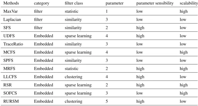
Table1summarizes a comparative study of the well-known feature selection algorithms based on their theoretical
90
proprieties: (1) their categories, (2) the classes of the used filters (statistic, similarity, etc.), (3) the number of user-input
91
parameters, (4) the level of sensibility to parameters values changes, (5) the scalability.
92
Table 1: Comparison of various feature selection algorithms corresponding to their theoretical proprieties.
Methods category filter class parameter parameter sensibility scalability
MaxVar filter statistic 1 low high
Laplacian filter similarity 3 low low
SFS filter similarity 2 high low
UDFS Embedded sparse learning 4 high low
TraceRatio Embedded similarity 3 low low
MCFS Embedded sparse learning 4 low high
SPFS Embedded similarity 3 low low
MRFS Embedded statistic 2 high high
LLCFS Embedded clustering 4 high low
RSR Embedded sparse learning 2 high high
SOFCS Embedded sparse learning 3 low high
RURSM Embedded clustering 5 high low
2.2. Subspace and projected algorithms 93
Subspace learning algorithms have been proposed to cope with the various curse of dimensionality aspects (Li 94
et al.,2011), such (1) the distances concentration problem, where geometrical distances gave insignificant differences
95
between different pairs of samples and (2) the hubness phenomenon related to the distance concentration problem,
96
which affects the distribution of k-occurrences (Flexer & Schnitzer,2015)
97
Indeed, a pair (C,S) is selected, whereCis a set of points composing a cluster andS is a set of the most
char-98
acterizing features of the considered cluster. CLIQUE is a subspace clustering algorithm based on grid (Böhm et al.,
99
2004). Based on an Apriori-like method, it recursively searches the set of all possible subspaces. It used a density
threshold to filter cells. Based on conclusions given byFlexer & Schnitzer(2015) which demonstrated that Euclidian
101
distances are not efficient,Böhm et al.(2004) proposed a weighted Euclidian distance based on subspace concepts
102
and the well-founded notion of density connected clusters. Authors proposed the use of subspace preference cluster
103
concepts, based on the variance of the data neighborhood along features, then weighted the Euclidian distance by
104
these variances (more details are given in Section3).
105
2.3. Graph centrality measures 106
The growth of social networks and web services motivated the centrality measures researches. Several points of
107
view have been proposed to evaluate node importance in a graph. In ‘Degree Centrality’, node importance is the
108
number of its directly connected edges. ‘Closeness Centrality’ (Opsahl et al.,2010) used distances between nodes
109
and lower values reflect information on the graph. The ‘Betweenness Centrality’ (Opsahl et al.,2010) highly scored
110
nodes communicated to others with few intermediaries. The ‘Eigenvector centrality’ (Opsahl et al.,2010) reflected
111
the number of connections with nodes strongly connected with other graph actors. Google has proposed an efficient
112
measure based on Eigenvector centrality called ‘PageRank’ to investigate web pages relevance (Gleich,2015). This
113
simple and fast measure is general and well-defined for any given graph structure to capture various relations among
114
nodes. PageRank has been applied in biology and bioinformatics to find and rank genes ‘GeneRank’ (Morrison 115
et al.,2005), proteins ‘ProteinRank’ (Wu et al.,2013) or even to match protein-protein interactions (IsoRank). It is
116
also used in neuroscience, complex engineered systems (MoniorRank), in the Linux kernel, bibliometrics (CiteRank,
117
TimedPageRank,AuthorRank), in social networks (SuperedgeRank(Ma & Liu,2014),BuddyRankandTwitterRank)
118
as well as in other contexts (Gleich,2015).
119
3. Mathematical Framework
120
This section first presents notations then recalls the bases of subspace learning and PageRank.
121
3.1. Notations 122
LetX be a set ofnpoints andd−dimensional features X = {x1, . . . ,xn}. Each pointxiis a vector ofd features
123
xi=(x1i, . . . ,xdi).dist(xp,xq) is the Euclidean distance between two data pointsxp,xq∈Xand thedistp:X×X→R 124
is a metric distance function between projected points.
125
Our aim is to develop a new feature selection algorithm which maps features into an undirected graph. Let
126
G =<V,E >a graph, where the vertices (nodes)Vare the set of featuresV ={x1, . . . ,xd}, andEthe edges linking
127
the vertices. Ais the adjacency matrix associated to the graphG, where each of its elementai,jrepresents a pairwise 128
relationship between featuresxiandxj.a
i,jis associated to a potential functionφ(xi,xj) : 129
ai,j=φ(xi,xj) (1)
The functionφcan be a binary function as it can weight nodes composing the graph via several metrics.
3.2. Subspace preference clusters 131
Several studies have demonstrated the capacity of subspace preference to deal with high-dimensional spaces ( El-132
hamifar & Vidal,2013; Parsons et al.,2004;Vidal,2011; Böhm et al.,2004). In this study, we use the subspace
133
preference clusters among features (Böhm et al.,2004) to define relationships between features.
134
Subspace preference cluster is a set of points belonging to the same dense regions called ‘density connected
135
points’, which are associated to a set of features called ‘subspace preference vector’. Subspace preference clusters are
136
sets of points with small variance along one or more features, i.e. a variance smaller than a given thresholdδ∈R.
137
Letxp∈Xa data point andk∈N. The variancevari(NNk(xp)) along a featurexiis defined as follows:
138 vari(NNk(xp))= P xq∈NNk(xp)(distp(x i p,xiq)) 2 |NNk(xp)| (2) whereNNk(xp) define the set ofk−nearest neighborhoods of an objectxp∈X.
139
The feature subspace preference associated to the data pointxp∈Xis the set of features withvari(NNk(xp))≤δ,
140
δ∈R,k ∈N. This features set preserves the density in the neighborhood of the pointxp. Therefore, if the selected
141
set of features (subspace preference cluster) has low variance in the neighborhood of points, thus those features are
142
relevant and preserve the density inside the cluster of the data pointxp.
143
3.3. PageRank 144
The PageRank measure has been introduced originally by Google to rank web-pages. It simulated the behavior
145
of users when browsing the Web to rank pages, where pages are graph nodes and hyperlinks are edges. PageRank
146
denotes the ‘importance’ of nodes under the assumptions that the importance of a node is the expected sum of the
147
importance of all connected nodes and the direction of edges. Its value corresponds to the probability distribution of
148
nodes being accessed at random. In graph theory, PageRank computes recursively a normalized and propagated value
149
for each node in a graph.
150
Letxandptwo nodes in a graphG, the PageRank ofxis given as follows:
151
PR(x)=(1−c)+c. X p∈Pntin(x)
PR(p)
|Pntout(p)| (3)
wherecis a damping factor which takes its value in [0,1] (typically 0.85),Pntin(x) is the set of nodes pointing to 152
xandPntout(p) the set of nodes pointed bypand|Pntout(p)|is its cardinality. The PageRank operated on the directed
153
graph and its value for a given node is computed iteratively based on PageRank of nodes pointing on it. In order to
154
deal with undirected graphs, some variants of PageRank have been proposed (Avrachenkov et al.,2015;Zhang et al.,
155
2016). In our study, we used the basic version of the algorithm. The PageRank vector is a stationary distribution of
156
special formed Markov process, more details about its convergence are given in (Gleich,2015).
4. Usupervised Graph-based Feature Selection method ‘UGFS’
158
The purpose of this work consists in investigating the importance of features in an undirected graph using
PageR-159
ank. It highlights nodes (feature) having a lot of connections. The graph design is a crucial step because features
160
must be connected with respect to PageRank proprieties. We use the subspace preference clusters in order to define
161
the edges linking features. Features relationships are defined according to their abilities to preserve the neighborhood
162
densities of data points, i.e., features minimizing variances among projected neighborhood data of each core data
163
point are linked.
164
In order to define feature relationships, the proposed algorithm scans the whole dataset searching the neighborhood
165
of each data point. Then, it computes the variances among these sets. Based on a given threshold and the computed
166
variances (see section3.2), the algorithm selects subspace preference clusters for each data point. Features belonging
167
to the same subspace preference clustersSpassociated to the neighborhood of the pointxpare linked. Otherwise,
168
if the subspaceSp preserves the local densities into the projected neighborhoods of the data pointxp, then features
169
composingSp are the most relevant for the cluster ofxp. That is, the edges linking those features must be created.
170
The potential function associated to the graphGis given by:
171 φ(xi,xj)= 1, ifvarsp(NNk(xp))≤δ 0, otherwise (4)
wherexi,xj ∈Spandδ∈Ris a variance threshold. 172
More details about the definition of feature relationships and graph design are given in algorithm13.
173
Finally, UGFS applies the PageRank system as a centrality measure of graphG, then features are ranked according
174
to their PageRank score.
175
5. Experimental Results
176
5.1. Experimental Setup 177
UGFS is implemented in the MATLAB R2017 software (The Mathworks Inc, Massachusetts, USA), under
Win-178
dows Operating System. Experimental evaluation is done on a laptop i5 Intel dual processor 2.3 GHz/CPU and 8 GB
179
DRAM.
180
The evaluation of the proposed algorithm are done by means of (1) the classification rate and its standard deviation
181
corresponding to feature subsets of different sizes are computed by a cross-validation representing 40% of the whole
182
dataset, (2) the minimum number of features corresponding to the best classification rates and (3) the redundancy rate
183
of the selected feature subsets.
184
Algorithm 1: Feature Graph design
Input: Observed dataX={x1, . . . ,xn},k,δ.
Output:Gundirected graph of features.
1: ComputeNNk(xi), withi=1, . . . ,n.
2: ComputeVarj(NNk(xi)), withi=1, . . . ,nand j=1, . . . ,d(see section3.2; equation2). 3: A(i,j)=0,i=1, . . . ,dandj=1, . . . ,d. 4: fori=1 :ndo 5: for j=1 :ddo 6: if Varj(NNk(xi))≤δthen 7: VarBinarized(i,j)=1 8: else 9: VarBinarized(i,j)=0 10: end if 11: end for 12: end for 13: fori=1 :ndo 14: Sp={} 15: for j=1 :ddo
16: ifVarBinarized(i,j)==1then
17: Sp=Sp∪ {xj} 18: end if 19: end for 20: forl=1 :size(Sp)do 21: form=1 :size(Sp)do 22: A(l,m)=1 23: end for 24: end for 25: end for 26: G=({x1, . . . ,xd},A)
The redundancy rate of a given feature subsetS, is given by:
185 RED(S)= 1 d(d−1) X xi,xj∈S,i>j corr(xi,xj) (5)
wheredis the size of feature dataset andxi,xj ∈S. Large values ofRED(s) means that features of the subsetS
186
are significantly correlated.
We use two classifiers: (1) the support vector machine (SVM) for supervised classification (Cortes & Vapnik,
188
1995), which is widely used both in feature selection algorithm design and/or evaluation and (2) thek−means for
189
unsupervised learning (Celebi et al.,2013), which is simple, fast and requires only the number of clusters as input
190
parameter.k−means initial centroids choice influences highly its accuracy, that is why we usek−means++algorithm
191
to choose the centroids initial values.
192
Best feature ranking is then demonstrated by minimization of the evaluation criteria, except the classification rate
193
where higher values indicated the features relevance and their ability to discriminate classes.
194
5.2. Comparison with feature selection methods 195
To validate the effectiveness of the proposed feature selection algorithm, we compare it with the following feature
196
selection methods:
197
• Laplacian Score: Selects features preserving the similarity of the original data (He et al.,2005).
198
• Unsupervised Discriminative Feature Selection (UDFS): Selects features by the local discriminative score and
199
preserves manifold structure (Yang et al.,2011).
200
• Local Learning-Based Clustering Feature Selection (LLCFS): Selects features by incorporating the feature
rel-201
evance evaluation into local learning-based clustering algorithm (Zeng & Cheung,2010).
202
• Correlation-based Feature Selection (CFS): Selects features corresponding to the minimum pairwise correlation
203
(Hall,2000).
204
• Spectral Feature Selection (SFS): Selects features using the spectrum information of the Laplacian graph (Zhao 205
& Liu,2007).
206
• Eigenvector Centrality for Feature Selection (ECFS): Ranks features by measuring the eigenvector centrality of
207
the pairwise features graph (Roffo & Melzi.,2017).
208
Note that, all these algorithms are unsupervised, except the ECFS, which analysis feature graph to rank them. We
209
compare UGFS with ECFS in order to validate the proposed graph design.
210
5.3. Dataset 211
We are interested in data scenarios where the dimensionality of the input space is much larger than the data size,
212
so-called High Dimension Low Sample Size (HDLSS) datasets (Zhang & Lin,2013). Most of machine learning
213
algorithms are less efficient when dealing with such data, which emerged these days, particularly in bioinformatics
214
where gene/expression datasets are HDLSS. We used 4 open access datasets4: Colon, leukemia, ovarian cancer and 215
CLL_SUB_111 described in Table2.
216
Table 2: Datasets description
Datasets Number of features Number of Instances Number of classes
Colon 2000 62 2
Leukemia 7129 72 2
Ovarian cancer 4000 216 2
CLL_SUB_111 11340 111 3
5.4. Results and discussion 217
We compared the developed method (UGFS) to different feature selection methods (Laplacian Score, UDFS,
218
LLCFS, CFS, SFS, and ECFS) using the 4 datasets. Figure1,2,3and4represent the classification rate according to
219
the number of selected features, when we used an SVM (Figure1.(a),2.(a),3.(a) and4.(a) and ak−means algorithm
220
(Figure1.(b),2.(b),3.(b) and4.(b)). We notice that on most of cases the classification rate decreases as the number of
221
feature increases. In other words, feature selection algorithms improve the accuracy of learning algorithms by using
222
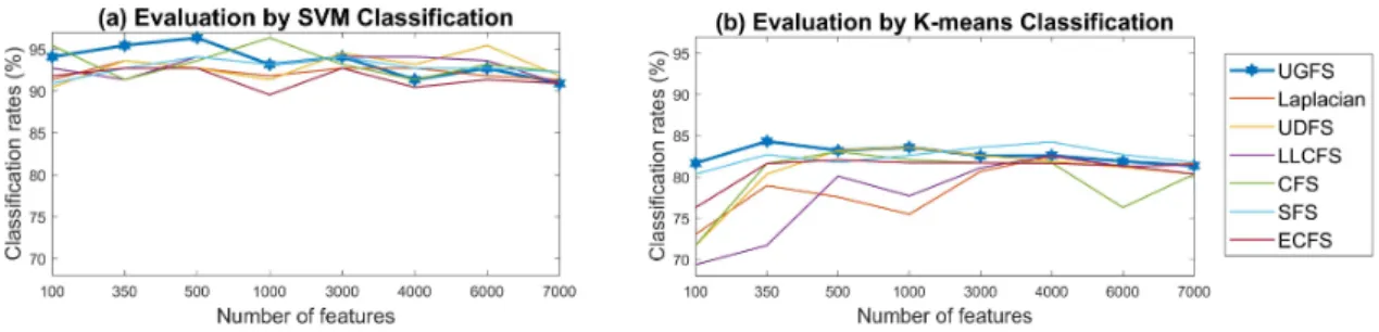
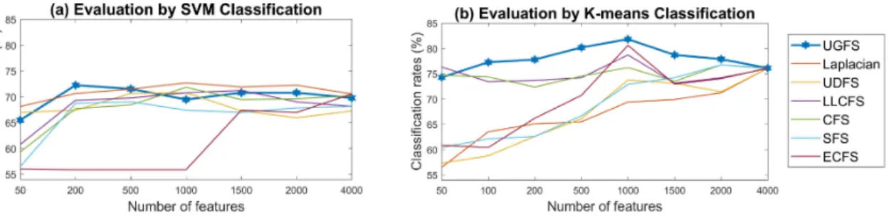
only relevant features and improve also the computational time.
223
Figure 1: Colon dataset: correct classification rate (%) of different feature selection algorithms, over a varied number of features.
Figure 2: leukemia dataset: correct classification rate (%) of different feature selection algorithms, over a varied number of features.
The effectiveness of the UGFS method to highly score the relevant features is demonstrated for both SVM and
224
k-means classifiers, where we obtain high classification rates for the firsts features (150 features for colon datasets and
225
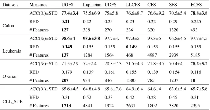
500 for both leukemia and ovarian cancer). These results are confirmed in Table3and4, where we summarized the
226
classification rate (ACC), the standard deviation (STD), the redundancy rate (RED) and the selected number of features
Figure 3: Ovarian cancer dataset: correct classification rate (%) of different feature selection algorithms, over a varied number of features.
Figure 4: CLL_sub_111 dataset: correct classification rate (%) of different feature selection algorithms, over a varied number of features.
(# features). We notice that considering the smallest number of features and the stability of the classification rate (via
228
STD values), classifiers based on UGFS ranking obtain, generally, good classification rate and a low redundancy rate.
229
The ECFS algorithm, which is a supervised method, allows in most cases the best classification rate. However,
230
it uses usually a large number of features. Therefore, it is not efficient in ranking relevant features. Table3depicts
231
that ECFS allows an SVM classification rate of 78.17% using only 10 features. This result is perfect both in terms
232
of classification rate and the number of features. However, in gene/expression data analysis, the use of only 10 genes
233
from 4000 to describe 216 tissues is too restrictive. Therefore, comparisons of UGFS and ECFS show the efficiency
234
of UGFS in dimensionality reducing while retaining the relevant features, which confirms the importance of the graph
235
design in the feature ranking by centrality measure.
236
Note that, in this study, the considered datasets are real-world data characterized by low linear correlations between
237
their features. This explains the small variations in the redundancy rates based essentially on linear pairwise feature
238
correlations (Table3and4).
239
In order to assess the differences between UGFS and other methods regarding the size of the retained features
240
subsets (reported in Table3and4), a statistical analysis was performed by the paired samples Wilcoxon test. In all
241
cases, the statistical analysis shows a significant difference between UGFS and other methods.
Table 3: Comparison of different feature selection methods using SVM classifiers.
Datasets Measures UGFS Laplacian UDFS LLCFS CFS SFS ECFS
Colon ACC(%)±STD 77.4±3.4 75.5±6.9 75±5.8 76.6±8.7 76.6±9.2 70.5±5.4 78.8±3.8 RED 0.21 0.22 0.23 0.23 0.22 0.29 0.225 # Features 127 338 270 236 320 1320 493 Leukemia ACC(%)±STD 98.6±4 98.6±3.8 97.7±4. 97.3±5 97.3±5 96.8±4.5 97.7±4.5 RED 0.149 0.155 0.155 0.149 0.155 0.155 0.155 # Features 137 1284 1564 468 4987 2939 5185 Ovarian ACC(%)±STD 71.5±2.9 72±2.4 70.8±7.3 71.5±4.3 71.8±3.7 70.4±4 78.2±5.2 RED 0.179 0.139 0.161 0.155 0.139 0.154 0.116 # Features 207 984 846 1300 785 1237 10 CLL_SUB ACC(%)±STD 65.8±4.5 64.8±4.8 65.6±7.8 64.9±6.4 64.6±4 63.6±5.4 65.7±5.8 RED 0.31 0.52 0.38 0.42 0.28 0.45 0.31 # Features 1713 4841 1924 2631 1802 3820 2395
Table 4: Comparison of different feature selection methods usingk-means classifiers.
Datasets Measures UGFS Laplacian UDFS LLCFS CFS SFS ECFS
Colon ACC(%)±STD 80.4±3 78.7±2.9 79.5±2.8 78.7±2.9 79.5±2.9 79.7±2.8 82.35±3.3 RED 0.23 0.24 0.225 0.23 0.2 0.247 0.24 # Features 213 479 257 349 250 1341 575 Leukemia ACC(%)±STD 91.3±4.3 88.2±5.2 90.3±4.2 87.7±4.8 86.8±4.6 79.1±6.1 86.6±5.4 RED 0.141 0.145 0.148 0.152 0.153 0.15 0.143 # Features 338 1400 486 5860 6591 5610 509 Ovarian ACC(%)±STD 83.75±5.2 73.5±5.7 80.7±4.9 81.2±4.7 79.2±6.1 78.9±5.9 84.2±5.9 RED 0.164 0.21 0.234 0.55 0.25 0.512 0.175 # Features 280 548 659 1382 692 1245 315 CLL_SUB ACC(%)±STD 51.3±7.5 55.6±8.2 49.8±8.8 51.4±8.4 50.6±7.1 45.6±7.5 49.6±8.1 RED 0.3 0.49 0.375 0.4 0.25 0.47 0.34 # Features 1626 4754 1894 2415 1756 3884 2045
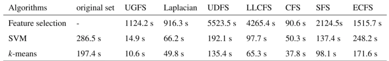
In order to investigate the implications of feature selection algorithms in terms of runtime, we have generated a
243
big dataset in a high dimensional space (10000 objects and 7000 features), and we have compared the runtime of the
244
feature selection algorithms as well as the runtime of classification methods (SVM andk-means) for classifying the
245
original dataset and the reduced dataset (only the features given the best classification rates are considered).
Table.5summarizes the obtained runtime of all algorithms. First, we note that filter methods are the faster ones,
247
for instance, the CFS algorithm, which ranks features based only on their pairwise correlation, have needed just 90,6
248
s to perform ranking. However, embedded methods such UGFS and LLCFS, are slower but support classifiers (SVM
249
andk-means) to speed up the classification runtime while obtaining better accuracies.
250
Table 5: Comparison of the feature selection and the classification runtime.
Algorithms original set UGFS Laplacian UDFS LLCFS CFS SFS ECFS
Feature selection - 1124.2 s 916.3 s 5523.5 s 4265.4 s 90.6 s 2124.5s 1515.7 s
SVM 286.5 s 14.9 s 66.2 s 192.1 s 97.7 s 50.3 s 137.4 s 248.2 s
k-means 197.4 s 10.6 s 49.8 s 135.4 s 65.3 s 37.8 s 98.1 s 171.6 s
To summarize, UGFS is a graph-based method for an unsupervised feature selection, it needs only one parameter
251
which can be estimated from data distribution. It is a multivariate method, which leads to a higher effectiveness in
252
selecting discriminative features. However, this method is slower compared to the filter methods (univariate and less
253
effective feature selection methods). Indeed, it is executed in an iterative processing.
254
6. Conclusion
255
This paper proposes a novel unsupervised feature selection method based on graph and subspace concepts.
Fea-256
tures are mapped in an undirected graph using subspace learning, where data manifold structure is preserved. We used
257
the prestigious Google’s PageRank system as a centrality measure for ranking features by means of their importance
258
and topological roles in the graph. Graph-based methods and centrality measures exploit the feature combination
259
potential, although their effectiveness depends on the graph design. Therefore, we defined in this paper a novel
fea-260
ture relationships measure based on subspace learning, it linked the features which their interaction discriminated the
261
classes. Then, PageRank assigned higher scores for the most relevant features and found the smallest feature subset
262
guaranteeing the best precision.
263
Experimental results on real-world high dimension low sample size datasets demonstrate the effectiveness of our
264
method (UGFS) against the existing unsupervised algorithms. The subsets selected by UGFS are almost the smallest,
265
and they support classifiers to achieve higher classification rates in a lower runtime.
266
In the future, we plan to further investigate the following aspects of UGFS: 1) the graph direction will be
consid-267
ered and constraints will be added to avoid outliers and noisy data. 2) UGFS has one parameter to tune, therefore we
268
plan to investigate the density threshold tuning and use a learning method such as ’association rules’ to extract feature
269
relationships. 3) This paper initiated the study of feature relationships in terms of their relevance, unlike traditional
270
methods which considered the features redundancy. This allows the future consideration of advanced feature
rela-271
tionship measures. 4) For UGFS applications in intelligent systems, it can benefit from the domain knowledge, for
272
instance, the use of ontologies knowledge in the graph design. 5) The use of the UGFS algorithm with state-of-the-art
classifiers such as the convolutional neural network. These methods require a large database, however, this limitation
274
could be overcome using transfer learning.
275
7. Acknowledgements
276
This research was supported in part by the program MITACS, accelerate FR20930 and by the Canada research
277
chair on biomedical data mining (950-231214).
278
References
279
Abdi, H. & Williams, L. J. (2010). Principal component analysis.Wiley Interdisciplinary Reviews: Computational Statistics, 2(4), 433–459.
280
Aliyari, G. Y., Rudzicz, F., & Moghaddam, H. A. (2015). Fast incremental LDA feature extraction.Pattern Recognition, 48(6), 1999–2012.
281
Avrachenkov, K., Kadavankandy, A., Prokhorenkova, L. O., & Raigorodskii, A. (2015). Pagerank in undirected random graphs. InLecture Notes 282
in Computer Science (including subseries Lecture Notes in Artificial Intelligence&Lecture Notes in Bioinformatics), 9479, 151–163.
283
Bennasar, M., Hicks, Y., & Setchi, R. (2015). Feature selection using joint mutual information maximisation.Expert Systems with Applications,
284
42(22), 8520–8532.
285
Böhm, C., Kailing, K., Kriegel, H.-P., & Kroger, P. (2004). Density connected clustering with local subspace preferences. InProceedings of the 286
Fourth IEEE International Conference on Data Mining, ICDM ’04, Washington, DC, USA(pp. 27–34).
287
Cai, D., Zhang, C., & He, X. (2010). Unsupervised feature selection for multi-cluster data. InProceedings of the 16th ACM SIGKDD international 288
conference on Knowledge discovery&data mining - KDD ’10(pp. 333–342).
289
Celebi, M. E., Kingravi, H. A., & Vela, P. A. (2013). A comparative study of efficient initialization methods for the k-means clustering algorithm.
290
Expert Systems with Applications, 40(1), 200–210.
291
Choi, H. & Choi, S. (2007). Robust kernel Isomap.Pattern Recognition, 40(3), 853–862.
292
Cortes, C., & Vapnik, V. (1995). Support vector machine.Machine learning, 20(3), 1303–1308.
293
Du, S., Ma, Y., Li, S., & Ma, Y. (2017). Robust unsupervised feature selection via matrix factorization.Neurocomputing, 241(C), 115–127.
294
Duda, R. O., Hart, P. E., & Stork, D. G. (2001). Pattern classification. 2nd. Edition.Wiley-Interscience, New York, USA.
295
Elhamifar, E., & Vidal, R. (2013). Sparse Subspace Clustering: Algorithm, Theory, & Applications. IEEE Transactions on Pattern Analysis& 296
Machine Intelligence, 35(11), 2765–2781.
297
Flexer, A., & Schnitzer, D. (2015). Choosing`pnorms in high-dimensional spaces based on hub analysis.Neurocomputing, 169, 281–287.
298
Gleich, D. F. (2015). PageRank beyond the Web.Society for Industrial&Applied Mathematics, 57(3), 321–363.
299
Hall, M. A. (2000). Correlation-based feature selection for discrete & numeric class machine learning. InProceedings of the Seventeenth Interna-300
tional Conference on Machine Learning, ICML ’00, San Francisco, CA, USA(pp. 359–366).
301
Han, D. & Kim, J. (2015). Unsupervised Simultaneous Orthogonal basis Clustering Feature Selection. InProceedings of the IEEE Computer 302
Society Conference on Computer Vision&Pattern Recognition(pp. 5016–5023).
303
Hassani, M., Kim, Y., Choi, S., & Seidl, T. (2014). Subspace clustering of data streams: new algorithms & effective evaluation measures.Journal 304
of Intelligent Information Systems, 45(3), 319–335.
305
He, X., Cai, D., & Niyogi, P. (2005). Laplacian Score for Feature Selection. InProceedings of the 18th International Conference on Neural 306
Information Processing Systems, NIPS’05, Vancouver, BC, Canada (pp. 507–514).
307
Hu, L., Gao, W., Zhao, K., Zhang, P., & Wang, F. (2018). Feature selection considering two types of feature relevancy & feature interdependency.
308
Expert Systems with Applications, 93(C), 423–434.
309
Krzanowski, W. J. (1987). Selection of variables to preserve multivariate data structure using principal components.Journal of the Royal Statistical 310
Society. Series C (Applied Statistics), 36(1), 22–33.
Li, Y., Hung, E., & Chung, K. (2011). A subspace decision cluster classifier for text classification. Expert Systems with Applications, 38(10),
312
12475–12482.
313
Ma, N. & Liu, Y. (2014). Superedgerank algorithm & its application in identifying opinion leader of online public opinion supernetwork.Expert 314
Systems with Applications, 41(4, Part 1), 1357–1368.
315
Martinez-Gonzalez, B., Pardo, J. M., Echeverry-Correa, J. D. & San-Segundo, R. (2017). Spatial features selection for unsupervised speaker
316
segmentation and clustering.Expert Systems with Applications, 73, 27–42 .
317
Moradi, P. & Rostami, M. (2015). A graph theoretic approach for unsupervised feature selection.Engineering Applications of Artificial Intelligence,
318
44(Supplement C), 33–45.
319
Morrison, J. L., Breitling, R., Higham, D. J., & Gilbert, D. R. (2005). GeneRank: using search engine technology for the analysis of microarray
320
experiments.BMC bioinformatics, 6(1), 233.
321
Nie, F., Xiang, S., Jia, Y., Zhang, C., & Yan, S. (2008). Trace Ratio Criterion for Feature Selection. InProceeding of the Twenty-Third AAAI 322
Conference on Artificial Intelligence, AAAI’08,Chicago, Illinois, USA(pp. 671–676).
323
Opsahl, T., Agneessens, F., & Skvoretz, J. (2010). Node centrality in weighted networks: Generalizing degree & shortest paths.Social Networks,
324
32(3), 245–251.
325
Parsons, L., Haque, E., & Liu, H. (2004). Subspace clustering for high dimensional data.ACM SIGKDD Explorations Newsletter, 6(1), 90–105.
326
Roffo, G. & Melzi, S. (2017). Ranking to Learn: Feature Ranking & Selection via Eigenvector Centrality. InNew Frontiers in Mining Complex 327
Patterns(pp. 1–15).
328
Somol, P., Baesens, B., Pudil, P., & Vanthienen, J. (2005). Filter- versus wrapper-based feature selection for credit scoring.International Journal 329
of Intelligent Systems, 20(10), 985–999.
330
Vidal, R. (2011). Subspace Clustering.IEEE Signal Processing Magazine, 28(2), 52–68.
331
Wu, G., Zhang, Y., & Wei, Y. (2013). Accelerating the Arnoldi-type algorithm for the PageRank problem & the ProteinRank problem.Journal of 332
Scientific Computing, 57(1), 74–104.
333
Yang, Y., Shen, H. T., Ma, Z., Huang, Z., & Zhou, X. (2011).`2,1-Norm regularized discriminative feature selection for unsupervised learning. In
334
IJCAI International Joint Conference on Artificial Intelligence(pp. 1589–1594).
335
Zeng, H. & Cheung, Y.-M. (2010). Feature Selection & Kernel Learning for Local Learning Based Clustering. IEEE transactions on pattern 336
analysis&machine intelligence, 33(8), 1532–1547.
337
Zhang, H., Li, F., Liu, P., Chen, Y., Ren, D., & Wang, K. (2017). How can a sparse representation be made applicable for very low-dimensional
338
data?.Expert Systems with Applications, 77(c), 66–70.
339
Zhang, H., Lofgren, P., & Goel, A. (2016). Approximate Personalized PageRank on Dynamic Graphs. InProceedings of the 22nd ACM SIGKDD 340
International Conference on Knowledge Discovery&Data Mining, KDD ’16(pp. 1315–1324).
341
Zhang, L. & Lin, X. (2013). Some considerations of classification for high dimension low-sample size data. Statistical Methods in Medical 342
Research, 22(5), 537–550.
343
Zhao, Z. & Liu, H. (2007). Spectral feature selection for supervised & unsupervised learning. InProceedings of the 24th international conference 344
on Machine learning - ICML ’07(pp. 1151–1157).
345
Zhao, Z., Wang, L., Liu, H., & Ye, J. (2013). On similarity preserving feature selection.IEEE Transactions on Knowledge&Data Engineering,
346
25(3), 619–632.
347
Zheng, Z., Lei, W., & Huan, L. (2010). Efficient Spectral Feature Selection with Minimum Redundancy. InTwenty-Fourth AAAI Conference on 348
Artificial Intelligence(pp. 1–6).
349
Zhu, P., Zuo, W., Zhang, L., Hu, Q., & Shiu, S. C. (2015). Unsupervised feature selection by regularized self-representation.Pattern Recognition,
350
48(2), 438–446.