Multi-class ROC analysis from a
multi-objective optimisation perspective
Richard M. Everson and Jonathan E. Fieldsend
Department of Computer Science, University of Exeter, Exeter, EX4 4QF, UK
Abstract
The Receiver Operating Characteristic (ROC) has become a standard tool for the analysis and comparison of classifiers when the costs of misclassification are un-known. There has been relatively little work, however, examining ROC for more than two classes. Here we discuss and present an extension to the standard two-class ROC for multi-two-class problems.
We define the ROC surface for theQ-class problem in terms of a multi-objective
optimisation problem in which the goal is to simultaneously minimise theQ(Q−1)
misclassification rates, when the misclassification costs and parameters governing the classifier’s behaviour are unknown. We present an evolutionary algorithm to locate the Pareto front—the optimal trade-off surface between misclassifications of different types. The use of the Pareto optimal surface to compare classifiers is dis-cussed and we present a straightforward multi-class analogue of the Gini coefficient. The performance of the evolutionary algorithm is illustrated on a synthetic three
class problem, for bothk-nearest neighbour and multi-layer perceptron classifiers.
Key words: receiver operating characteristic, evolutionary computation, multiple objectives, Pareto optimality, Gini coefficient.
1 Introduction
Classification or discrimination of unknown exemplars into two or more classes based on a ‘training’ dataset of examples, whose classification is known, is one
Email address: {R.M.Everson,J.E.Fieldsend}@exeter.ac.uk(Richard M. Everson and Jonathan E. Fieldsend).
of the fundamental problems in supervised pattern recognition. Given a classi-fier that yields estimates of the exemplar’s probability of belonging to each of the classes and when the relative relative costs of misclassification are known, it is straightforward to determine the decision rule that minimises the average cost of misclassification. If the cost of misclassification is taken to be 1 and there is no penalty for a correct classification then the optimal rule becomes: assign to the class with the highest posterior probability. In practical situa-tions, however, the true costs of misclassification are unequal and frequently unknown or difficult to determine [e.g. Bradley, 1997; Adams and Hand, 1999]. In such cases the practitioner must either guess the misclassification costs or explore the trade-off in classification rates as the decision rule is varied.
Receiver Operating Characteristic (ROC) analysis provides a convenient graph-ical display of the trade-off between true and false positive classification rates for two class problems [Provost and Fawcett, 1997]. Since its introduction in the medical and signal processing literatures [Hanley and McNeil, 1982; Zweig and Campbell, 1993] ROC analysis has become a prominent method for select-ing an operatselect-ing point; see [Flach et al., 2003] and [Hern´andez-Orallo et al., 2004] for a recent snapshot of methodologies and applications.
In this paper we extend the spirit of ROC analysis to multi-class problems by considering the trade-offs between the misclassification rates from one class into each of the other classes. Rather than considering the true and false pos-itive rates, we consider the multi-class ROC surface to be the solution of the multi-objective optimisation problem in which these misclassification rates are simultaneously optimised. Srinivasan [1999] has discussed a similar formula-tion of multi-class ROC, showing that if classifiers forQclasses are considered to be points with coordinates given by their Q(Q−1) misclassification rates, then optimal classifiers lie on the convex hull of these points. Here we describe the surface in terms of Pareto optimality and in section 3 we give an evolu-tionary algorithm for locating the optimal ROC surface when the classifier’s parameters may be adjusted as part of the optimisation. Since multi-class ROC surfaces live in Q(Q−1) dimensions visualisation is problematic, even for Q = 3; in section 4 we therefore consider visualisation methods for ROC surfaces for a probabilistic k-nearest neighbour (k-nn) classifier [Holmes and Adams, 2002] and a multi-layer perceptron classifying synthetic data.
ROC analysis is frequently used for evaluating and comparing classifiers, the area under the ROC curve (AUC) or, equivalently, the Gini coefficient. Al-though the straightforward analogue of the AUC is unsuitable for more than two classes, in section 5 we develop a straightforward generalisation of the Gini coefficient which quantifies the superiority of a classifier’s performance to random allocation.
2 ROC Analysis
Here we describe the straightforward extension of ROC analysis to more than two classes (multi-class ROC) and draw some comparisons with the two class case.
In general a classifier seeks to allocate an exemplar or measurement x to one of a number of classes. Allocation of x to the incorrect class, say Aj,
usually incurs some, often unknown, cost denoted by λkj; we count cost a
correct classification as zero: λkk = 0. Denoting the probability of assigning
an exemplar to Aj when its true class is in fact Ak as p(Aj| Ak) the overall
risk or expected cost is
R =X
j,k
λkjp(Aj| Ak)πk (1)
where πk is the prior probability of Ak. The performance of some particular
classifier may be conveniently be summarised by a confusion matrix or contin-gency table, ˆC, which summarises the results of classifying a set of examples. Each entry ˆCkj of the confusion matrix gives the number of examples, whose
true class was Ak, that were actually assigned toAj. Normalising the
confu-sion matrix so that each row sums to unity gives the confuconfu-sion rate matrix, which we denote by C, whose entries are estimates of the misclassification probabilities:p(Aj| Ak)≈Ckj. Thus the expected risk is estimated as
R=X
j,k
λkjCkjπk. (2)
A slightly different perspective is gained by writing the expected risk in terms of the posterior probabilities of classification to each class. The conditional risk or average cost of assigning xtoAj is
R(Aj|x) =
X
k
λkjp(Ak|x) (3)
where p(Ak|x) is the posterior probability that x belongs to Ak. If α(x) is
a decision rule that assigns x to one of the classes Ak, then expected overall
risk associated with α is
R=
Z
R(α(x)|x)p(x)dx. (4)
The expected risk is then minimised, being equal to the Bayes risk, by as-signingxto the class with the minimum conditional risk [e.g. Duda and Hart, 1973]. Choosing ‘zero-one costs’,λkj = 1−δkj,means that all misclassifications
prob-ability; one thus assigns to the class with the greatest posterior probability, which minimises the overall error rate.
When the costs are known it is therefore straightforward to make assignments to achieve the Bayes risk (provided, of course, that the classifier yields accu-rate assessments of the posterior probabilities p(Ak|x)). However, costs are
frequently unknown and difficult to estimate, particularly when there are many classes; in this case it is useful to be able to compare the classification rates as the costs vary. For binary classification the conditional risk may be simply rewritten in terms of the posterior probability of assigning toA1, resulting in
the rule: assign x toA1 if P(A1|x)> t=λ12/(λ12+λ22). This classification
rule reveals that there is, in fact, only one degree of freedom in the binary cost matrix and, as might be expected, the entire range of classification rates for each class can be swept out as the classification thresholdt varies from 0 to 1. It is this variation of rates that the ROC curve exposes for binary classifiers. ROC analysis focuses on the classification of one particular class, say A1, and
plots the true positive classification rate for A1 versus the false positive rate
as the thresholdt or, equivalently, the ratio of misclassification costs is varied. If more than one classifier is available (often produced by altering the pa-rameters, w, of a particular classifier) then it can be shown that the convex hull of the ROC curves for the individual classifiers is the locus of optimum performance for that set of classifiers. [Provost and Fawcett, 1997, 1998] and Scott et al. [1998] have shown that performance at any point on the convex hull can be obtained by stochastically combining classifiers at the vertices of the convex hull.
Frequently in two class problems the focus is on a single class, for example, whether a set of medical symptoms are to be classified as benign or dangerous, so the ROC analysis practice of plotting of true and false positive rates for a single class has a direct physical interpretation. Also, since there are only three degrees of freedom in the binary confusion matrix, classification rates for the other class are easily inferred. Indeed, the confusionrate matrix,Chas only two degrees of freedom for binary problems. Focusing on one particular class is likely to be misleading when more than two classes are available for assignment. We therefore concentrate on the misclassification rates of each class to the others. In terms of the confusion rate matrix C we consider the off-diagonal elements, the diagonal elements (i.e., the true positives) being determined by the off-diagonal elements since each row sums to unity.
WithQclasses there areD=Q(Q−1) degrees of freedom in the confusion rate matrix and it is desirable to simultaneously minimise all the misclassification rates represented by these. For most problems, as in the binary problem, simultaneous optimisation will be impossible and some compromise between the various misclassification rates will have to be found. Knowledge of the costs
makes this determination simple, but if the costs are unknown we propose to use multi-objective optimisation to discover the optimal trade-offs between the misclassifications rates.
Since the units in which costs are measured are immaterial, the costs may, without loss of generality, be taken as summing to unity. We assume here that there is zero cost for correct assignment, λii= 0, so there are Q(Q−1)−1 = D−1 degrees of freedom for the specification of costs. Consequently, the op-timal trade-off surface between classification rates is, in general, of dimension
D−1, one fewer than the dimension of the ambient space and separates the origin of the [0,1]D hypercube from the (1, . . . ,1) corner. Locally the surface is parameterised by the (D−1) ratios of the misclassification costs in the same way that the binary ROC curve is parameterised byλ12/(λ12+λ21). To make
these ideas more precise we now define the optimal ROC surface in terms of a Pareto front.
In general we will consider locating the optimal ROC surface as a function of the classifier parameters,w, as well as the costs;wmight be, for example, the coefficients weighting the features in a linear discriminant or the weights of a neural network. For notational convenience and because they are treated as a single entity, we write the cost matrix λ and parameters as a single vector of generalised parameters, θ = {λ,w}; to distinguish θ from the classifier parameters w we use the optimisation terminology decision vectors to refer to θ. We consider the D misclassification rates to be functions (depending on the particular classifier) of the decision vectors, thus Ckj = Ckj(θ). The optimal trade-off between the misclassification rates is thus the defined by the minimisation problem:
minimise Ckj(θ) for all k, j. (5)
If the all misclassification rates for one classifier with decision vector θ are no worse than the classification rates for another classifierφ and at least one rate is better, then the classifier parameterised byθis said tostrictly dominate
that parameterised by φ. Thus θ strictly dominates φ (denoted θ ≺φ) iff:
Cjk(θ)≤Ckj(φ) ∀k, j and Ckj(θ)< Ckj(φ) for some k, j. (6)
Less stringently, θ weakly dominates φ (denoted θ φ) iff Ckj(θ) ≤Ckj(φ)
∀k, j.
A set E of decision vectors is said to be non-dominated if no member of the set is dominated by any other member:
A solution to the minimisation problem (5) is thusPareto optimal if it is not dominated by any other feasible solution, and the non-dominated set of all Pareto optimal solutions is known as the Pareto front. Recent years have seen the development of a number of evolutionary techniques based on dominance measures for locating the Pareto front; see Coello Coello [1999]; Deb [2001] and Veldhuizen and Lamont [2000] for recent reviews. Kupinski and Anasta-sio [1999] and AnastaAnasta-sio et al. [1998] introduced the use of multi-objective evolutionary algorithms (MOEAs) to optimise ROC curves for binary prob-lems, illustrating the method on a synthetic data set and for medical imaging problems; and we have used a similar methodology for locating optimal ROC curves for safety-related systems [Fieldsend and Everson, 2004; Everson and Fieldsend, 2006]. In the following section we describe a straightforward evolu-tionary algorithm for locating the Pareto front for multi-class problems. We illustrate the method on a synthetic problem for two different classification models in section 4.
3 Locating multi-class ROC surfaces
Here we describe a straightforward algorithm for locating the Pareto front for multi-class ROC problems using an analogue of mutation-based evolution. The procedure is based on the Pareto Archived Evolution Strategy (PAES) introduced by Knowles and Corne [2000]. In outline, the algorithm maintains a set or archive E of decision vectors, whose members are mutually non-dominating, which forms the current approximation to the Pareto front. As the computation progresses members of E are selected, copied and their decision vectors perturbed, and the objectives corresponding to the perturbed decision vector evaluated; if the perturbed solution is not dominated by any element of E, it is inserted into E and any members of E which are dominated by the new entrant are removed. Therefore the archive can only move towards the Pareto front: it is in essence a greedy search where the archive E is the current point of the search and perturbations toE that are not dominated by the current E are always accepted.
Algorithm 1 describes the procedure in more detail. The archiveEis initialised by evaluating the misclassification rates for a number (here 100) of randomly chosen parameter values and costs, and discarding those which are dominated by another element of the initial set. Then at each generation a single element,
θ is selected from E (line 3 of Algorithm 1); selection may be uniformly ran-dom, but partitioned quasi-random selection (PQRS) [Fieldsend et al., 2003] was used here to promote exploration of the front. PQRS prevents clustering of solutions in a particular region of the front biasing the search because they are selected more frequently, thus increasing the efficiency and range of the search.
Algorithm 1Multi-objective evolution scheme for ROC surfaces. Inputs:
T Number of generations
Nλ Number of costs to sample
1: E := initialise() 2: for t:= 1 :T
3: {w,λ}=θ:= select(E) PQRS
4: w0 := perturb(w) Perturb parameters
5: for i:= 1 :Nλ
6: λ0 := sample() Sample costs
7: C := classify(w0,λ0) Evaluate classification rates
8: θ0 :={w0,λ0}
9: if θ0 6φ ∀φ∈E
10: E :={φ∈E|φ⊀θ0} Remove dominated elements
11: E :=E∪θ0 Insert θ0
12: end
13: end
14: end
The selectedparent decision vector is copied, after which the costsλand clas-sifier parameters ware treated separately. The parameters w of the classifier are perturbed or, in the nomenclature of evolutionary algorithms, mutated, to form a child, w0 (line 4). Here we seek to encourage wide exploration of pa-rameter space by additively perturbing each of the papa-rameters with a random number δ drawn from a heavy tailed distribution (such as the Laplacian den-sity, p(δ) ∝ e−|δ|). The Laplacian distribution has tails that decay relatively slowly, thus ensuring that there is a high probability of exploring regions dis-tant from the current solutions, facilitating escape from local minima [Yao et al., 1999].
With a proposed parameter setw0 on hand the procedure then investigates the misclassification rates as the costs are varied with fixed parameters. In order to do this we generateNλ sample costs,λ
0
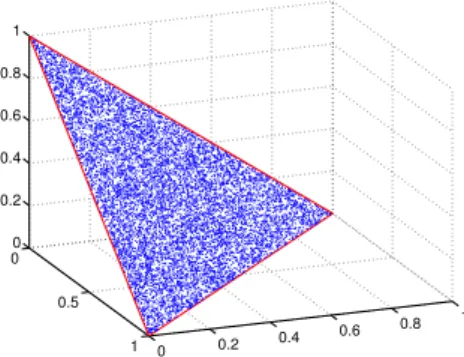
, and evaluate the misclassification rates for each of them. Since the misclassification costs are non-negative and sum to unity, a straightforward way of producing samples is to make a draws from a Dirichlet distribution:
p(λ) =Dir(λ|α1, . . . , αD) (8) = Γ( PD i=1αi) QD i=1Γ(αi) 1− D−1 X i=1 λi !αD−1D−1 Y i=1 λαi−1 i (9)
where the index i labels the D = Q(Q−1) off-diagonal entries in the cost matrix. As figure 1 illustrates, samples from a Dirichlet density lie on the simplex P
0 0.5 1 0 0.2 0.4 0.6 0.8 1 0 0.2 0.4 0.6 0.8 1
Figure 1. Samples from a 3-dimensional Dirichlet distribution, Dir(λ|1,1,1).
we have no preference for particular costs here, we set all the αkj = 1 so that
the simplex (that is, cost space) is sampled uniformly with respect to Lebesgue measure.
The misclassification rates for each cost sampleλ0 and classifier parametersw
are used to make class assignments for each example in the given dataset (line 7). Usually this step consists of merely modifying the posterior probabilities
p(Ak|x) to find the assignment with the minimum expected cost and is
there-fore computationally inexpensive as the probabilities need only be computed once for each w0. The misclassification rates Ckj(θ0) (j 6= k) comprise the
objective values for the decision vectorθ0 ={w0,λ} and decision vectors that are not dominated by any member of the archive E are inserted into E (line 11) and any decision vectors inE that are dominated by the new entrant are removed (line 10). We remark that this algorithm, unlike the original PAES algorithm, uses an archive whose size is unconstrained, permitting better con-vergence [Fieldsend et al., 2003]. Although at first sight unrestricted archives may appear to be computationally costly to store and query (as implied by lines 9 and 10), for realistic problems on modern machines storage is not con-straining and logarithmic time queries and updates can be achieved by the use of special data structures [Fieldsend et al., 2003]; in practice the main computational burden is usually evaluating the classification rates.
A (µ+λ) evolution strategy (ES) is defined as one in which µ decision vec-tors are selected as parents at each generation and perturbed to generate λ
offspring.2 The set of offspring and parents are then truncated or replicated
to provide theµparents for the following generation. Although Algorithm 1 is based on a (1 + 1)-ES, it is interesting to note that each parentθ is perturbed to yield Nλ offspring, all of whom have the classifier parameters w0 in
com-mon. With linear costs, evaluation of the objectives for many λ0 samples is inexpensive. Nonlinear costs could be incorporated in a straightforward man-ner, although it would necessitate complete reclassification for eachλ0 sample and it would therefore be more efficient to resample w with eachλ0.
2 We adhere to the optimisation terminology for (µ+λ)-ES, although there is a
x 1 x2 −1 −0.5 0 0.5 1 1.5 −0.2 0 0.2 0.4 0.6 0.8 1 1.2 1.4 1.6
Figure 2. Synthetic 3-class data. Magenta circles mark class 1, black triangles class 2 and yellow crosses class 3. Blue lines mark the optimal decision boundaries for equal misclassification costs.
4 Illustrations
In this section we illustrate the performance of the evolutionary algorithm on synthetic data, which is readily understood. Subsequently we give results for a number of standard multi-class problems. For simplicity we use two relatively simple classifiers, the k-nearest neighbour classifier (k-nn), which we now briefly describe in its probabilistic form [Holmes and Adams, 2002], and the multi-layer perceptron (MLP), a standard neural network.
4.1 Synthetic data
In order to gain an understanding of the Pareto optimal ROC surface for multiple class classifications we extend a two-dimensional, two-class synthetic data set devised by Ripley [1994] by adding additional Gaussian functions corresponding to an additional class. The resulting data set comprises 3 classes, the conditional density for each being a mixture of two Gaussians. Covariance matrices for all the components were isotropic: Σj = 0.3I. Denoting by µji
fori= 1,2 the means of the two Gaussian components generating samples for class j, the centres were located at:
µ11= (0.7,0.3)T µ12= (0.3,0.3)T
µ21= (−0.7,0.7)T µ22= (0.4,0.7)T (10)
µ31= (1.0,1.0)T µ32= (0.0,1.0)T
Each component had equal mixing weight 1/6. The 300 samples used here, together with the equal cost Bayes optimal decision boundaries, are shown in Figure 2.
4.2 Probabilistic k-nn
One of the most popular methods of statistical classification is the k-nearest neighbour model (k-nn). The method has a ready statistical interpretation, and has been shown to have an asymptotic error rate no worse than twice the Bayes error rate [Cover and Hart, 1967]. The method is essentially geometrical, assigning the class of an unknown exemplar to the class of the majority of its
k nearest neighbours in some training data. More precisely, in order to assign a datum x, given known classes and examples in the form of training data
D={yn,xn}Nn=1, thek-nn method first calculates the distances di =||x−xi||.
If theQclasses are a priori equally likely, the probability thatxbelongs to the
j-th class is then evaluated as p(Aj|x, k,D) = kj/k, where kj is the number
of the k data points with the smallestdn belonging to An.
Holmes and Adams [2002, 2003] have extended the traditional k-nn classifier by adding a parameterβ which controls the ‘strength of association’ between neighbours. The posterior probability of xbelonging to each classAj is given
by the predictive likelihood:
p(Aj|x, k, β,D) = exp[βPk xn∼xu(d(x,xn))δjyn] PQ q=1exp[β Pk xn∼xu(d(x,xn))δqyn] . (11)
Hereδmn is the Kronecker delta and Pkxn∼xmeans the sum over the k nearest
neighbours of x(excludingxitself). If the non-increasing function of distance
u(·) = 1/k, then the term Pk
xn∼xu(d(xn,x))δjyn counts the fraction of the k
nearest neighbours of x in the same class j as x. In the work reported here we chooseu to be the tricube kernel which gives decreasing weight to distant neighbours [Fan and Gijbels, 1996].
Holmes & Adams use the probabilistic formulation of the k-nn classifier as part of a Bayesian scheme in which they average over the parametersk andβ. Here we regardw={k, β}as parameters to be adjusted as part of Algorithm 1 as the Pareto optimal ROC surface is sought.
To discover the Pareto optimal ROC surface, the optimisation algorithm was run for T = 10000 proposed parameter values, with Nλ = 100, resulting in an estimated Pareto front comprising approximately 7500 mutually non-dominating parameter and cost combinations; we judge that the algorithm is very well converged and obtain very similar results by permitting the algorithm to run for only T = 2000 generations.
There are D = Q(Q−1) = 6 objectives to be minimised and, in common with other high-dimensional optimisation problems, visualisation of the 5-dimensional Pareto front is important for understanding the trade-offs possi-ble. A discussion of advanced visualisation techniques for this can be found in
x y −1 −0.5 0 0.5 1 1.5 −0.2 0 0.2 0.4 0.6 0.8 1 1.2 1.4 1.6 x y −1 −0.5 0 0.5 1 1.5 −0.2 0 0.2 0.4 0.6 0.8 1 1.2 1.4 1.6 x y −1 −0.5 0 0.5 1 1.5 −0.2 0 0.2 0.4 0.6 0.8 1 1.2 1.4 1.6
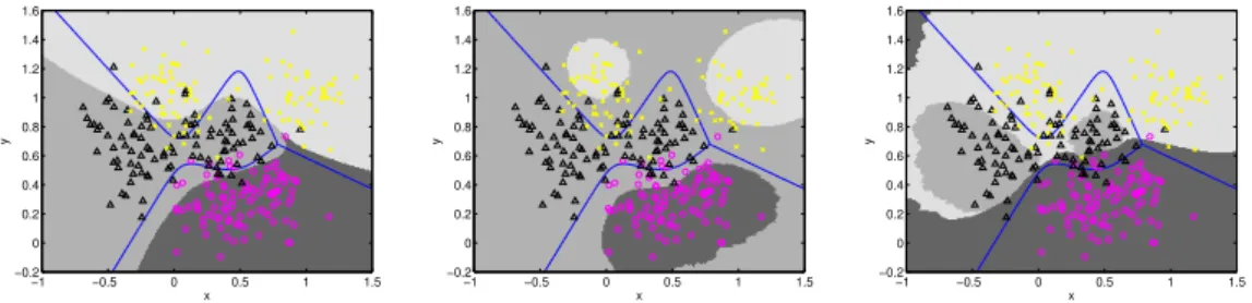
Figure 3. Decision regions for various k-nn classifiers on multi-class ROC surface.
Grey scale background shows the class to which a point would be assigned. Blue lines show the ideal equal-cost decision boundary. Symbols show actual training
data. Left: Parameters corresponding to minimum total misclassification error on
the training data. Middle: Decision regions corresponding to the minimum C21
and C23 and conditioned on this, minimum C31 and C13. Right: Decision regions
corresponding to minimising C12 and C32.
Fieldsend and Everson [2005b]
The left panel of the figure shows the decision regions that yield the smallest to-tal misclassification error, 32/300. This point has very similar decision regions to the equal-cost Bayes optimal ones, as might be expected since the overlap between classes is approximately comparable and there are equal numbers in each class. There are (3 in the results presented here) other parameterisations and cost combinations that also achieve this minimum misclassification rate. By contrast with the decision regions which are optimal for roughly equal costs, the middle and right panels of Figure 3 show decision regions for imbalanced costs. The middle panel shows a decision region corresponding to minimising
C21 andC23: this, of course, can be achieved by settingλ21andλ23 to be large,
so that everyA2 example (black triangle) is correctly classified, no matter what
the cost. For these data there are many decision regions correctly classifying every A2 and we display the decision regions that also minimise C31 and C13.
For these data, it is possible to make C31 = C13 = 0 because A1 and A3
are adjacent only along a boundary distant from A2 points; such complete
minimisation will in general not be possible. Of course, the penalty to be paid for minimising theA2 rates together withC31 and C13 is thatC32 andC12are
large: in fact, C32 > C12.
The right panel of Figure 3 shows the reverse situation: here the costs for misclassifying eitherA1 orA3 asC2 are high. With these data, although not
in general, of course, it is possible to reduce C12 and C32 to zero, as shown
by the decision regions which ensure that A2 examples (black triangles) are
only classified correctly when it does not result in incorrect assignment of the other two classes to A2. In this case the greatest misclassification rate is C23
4.3 Multi-layer perceptron classifiers
We also used a multi-layer perceptron (MLP) with a single hidden layer with 5 units and softmax output units as the classifier optimised by Algorithm 1. Again, the algorithm was run for T = 10000 evaluations of the classifier, re-sulting in an estimated Pareto front or ROC surface comprising approximately 4800 mutually non-dominating parameter and cost combinations. Note that for the MLP the parameter vectorwconsists of 33 weights and biases in con-trast to just two parameters for thek-nn classifier. In this case the archive was initialised by training a single MLP using quasi-Newton optimisation of the data likelihood [e.g. Bishop, 1995] which finds a point on or near the Pareto front corresponding to equal misclassification costs; subsequent iterations of the evolutionary algorithm are therefore largely concerned with exploring the Pareto front rather than locating it. Figure 4 shows decision regions for points on the Pareto front corresponding to those shown for the k-nn classifier in Figure 3.
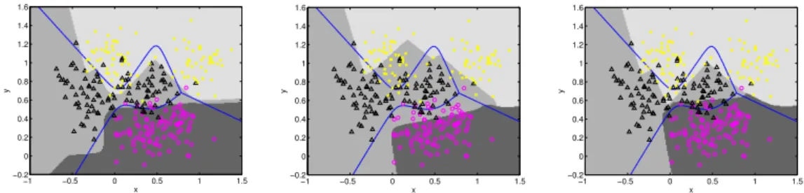
Decision regions corresponding to minimum overall misclassification error (Fig-ure 4, left) are similar to those for thek-nn classifier. The additional flexibility inherent in the MLP with 33 adjustable parameters permits the decision re-gions to be more finely tuned to the data: for example, theA2 (black triangles)
A3 (yellow crosses) boundary in Figure 4 lies to the right of the A2 data point
at (−0.456,1.21) so that it is correctly classified in contrast to thek-nn deci-sion regions in Figure 3. Although no explicit measures were taken to prevent over-fitting, the decision boundaries on the front are quite smooth and do not exhibit signs of over-fitting; permitting the optimisation algorithm to run for very long times might lead to over-fitting but we have not encountered it in the work reported here.
MLP decision regions minimisingC21, C23, C31 and C13, shown in the middle
panel of Figure 4 are similar to the k-nn regions (Figure 3) where the data density is high, but differ in detail where data are sparse. The same is true of the decision regions minimising misclassifications as A2, as can be seen by
comparing the right panels of Figures 3 and 4.
The decision regions illustrated in the middle and right panels of Figures 3 and 4 may thought of as lying on the edges of the Pareto surface because they correspond to one or more objectives being exactly minimised. These points are the analogues of the extreme ends of the usual two-class ROC curve where the false positive rate or the true positive rate is extremised. The curvature of the ROC curve in these regions is generally small, signifying that large changes in the costs yield large changes in either the true or false positive rate, but only small changes in the other. We observe a similar behaviour here: quite large changes theλkj in these regions yield quite small changes in the all the
x y −1 −0.5 0 0.5 1 1.5 −0.2 0 0.2 0.4 0.6 0.8 1 1.2 1.4 1.6 x y −1 −0.5 0 0.5 1 1.5 −0.2 0 0.2 0.4 0.6 0.8 1 1.2 1.4 1.6 x y −1 −0.5 0 0.5 1 1.5 −0.2 0 0.2 0.4 0.6 0.8 1 1.2 1.4 1.6
Figure 4. Decision regions for various MLP classifiers on multi-class ROC surface. Grey scale background shows the class to which a point would be assigned. Blue lines show the ideal equal-cost decision boundary. Symbols show actual training
data. Left: Parameters corresponding to minimum total misclassification error on
the training data. Middle: Decision regions corresponding to the minimum C21
and C23 and conditioned on this, minimum C31 and C13. Right: Decision regions
corresponding to minimising C12 and C32.
misclassification rates except the one which has been extremised, suggesting that the curvature of the Pareto surface is low in these areas.
A common use of the two-class ROC curve is to locate a ‘knee’, a point of high curvature. The parameters at the knee are chosen as the operational pa-rameters because the knee signifies the transition from rapid variation of true positive rate to rapid variation of false positive rate. Methods for numerically calculating the curvature of a manifold from point sets in more than two di-mensions are, however, not well developed (for a discussion, see Fieldsend and Everson [2005a]). Initial investigations in this direction have so far yielded only very crude approximations to the curvature in the 6-dimensional objec-tive space and we refrain from displaying them here. Although direct visual inspection of the curvature for multi-class problems is presently infeasible, we draw attention to the fact that the evolutionary algorithm yields a Pareto front of classifier parameterisations and associated costs.
4.4 False positive rates
Humans are particularly adept at visualisation in two and three dimensions, the intrinsic dimensions of the world we inhabit, and relatively inept at visu-alisation of high-dimensional objects. It is tempting therefore to attempt to reduce the dimension of the ROC surface sought so as to permit visualisa-tion. One straightforward way to achieve is to locate the trade-off surface for minimising misclassifications into each class, that is the false positive rate for each class. We minimise the Q objectives
Fk(w,λ) =
X
j6=k
0 0.2 0.4 0.6 0.8 1 0 0.2 0.4 0.6 0.8 1 0 0.2 0.4 0.6 0.8 1 F 2 F 1 F3
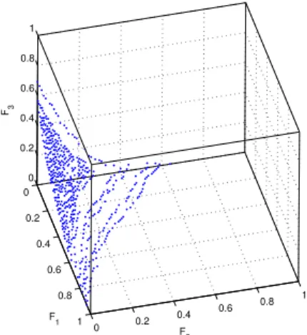
Figure 5. Estimated Pareto front where the objectives are the overall
misclassifica-tion rates for each class. Synthetic data usingk-nn classifiers.
The evolutionary algorithm is easily adapted to this minimisation problem and Figure 5 shows the Pareto surface obtained for the synthetic data, using the k-nn classifier and running the optimiser for T = 104 generations. We
call this front the ‘false positive rate front’ (similar to the true positive front described by Mossman [1999]). The figure shows the tradeoff between false positive rates for each of the three classes and a ‘corner’ or ‘knee’ can be located where all three misclassification rates are small and approximately equal. Decision regions for parameterisations close to the corner are similar to the equal-costs Bayes decision regions (Figure 2) and correspond to cost matrices, λ, with approximately equal entries. As may be expected the false positive rate for one class may be reduced, but, as the surface shows, only at the expense of raising the false positive rate for the other classes.
The false positive rate Pareto front is easily visualised (at least for three class problems), but information on exactlyhow misclassifications are made is lost. However, the full D-dimensional Pareto surface may usefully be viewed in ‘false positive space’. Figure 6 shows the solutions on the estimated Pareto front obtained using the full Q(Q−1) objectives for the k-nn classifier, but each solution is plotted as a grey scale symbol at the coordinate given by the
Q= 3 false positive rates (12), with the symbol grey scale denoting the class into which the greatest number of misclassifications are made.3 Although the solutions obtained by optimising the false positive rates directly lie on the full Pareto surface (in Q(Q− 1) dimensions) the converse is not true and the projections into false positive space do not form a surface. Nonetheless, at least for these data, they lie close to a surface, which aids visualisation and navigation of the full Pareto front. The relation between the solutions on the full Pareto front and the false positive rate front is made more precise as
3 A colour movie showing views from other angles can be found at http://www.
0 0.2 0.4 0.6 0.8 1 0 0.2 0.4 0.6 0.8 1 0 0.2 0.4 0.6 0.8 1 F 1 F 2 F3 0 0.2 0.4 0.6 0.8 1 0 0.2 0.4 0.6 0.8 1 0 0.2 0.4 0.6 0.8 1 F 1 F 2 F3 Predicted class Actual class 1 2 3 1 2 3
Figure 6. Two views of the estimated Pareto front for synthetic data classified with
a k-nn classifier viewed in false positive space. Axes show the false positive rates
for each class and points are coloured according to the class into which the greatest number of misclassifications are made, the overall misclassification rates for each class.
follows. IfE is a set ofQ(Q−1)-dimensional solutions lying in the full Pareto front, letEQbe the set ofQ-dimensional vectors representing the false positive
coordinates of elements of E. The extremal set of non-dominated elements of
EQ is
˜
EQ={f ∈EQ|f 6≺f0 ∈EQ}. (13)
Then solutions in ˜EQ also lie in the false positive rate front.
5 Comparing classifiers
In two class problems the area under the ROC curve (AUC) is often used to compare classifiers. As clearly explained by Hand and Till [2001], the AUC measures a classifier’s ability to separate two classes over the range of possible costs and is linearly related to the Gini coefficient. In this section we compare thek-nn and MLP classifiers using a measure based on the volume dominated by the Pareto optimal ROC surface.
By analogy with the AUC, we might therefore use the volume of theQ(Q− 1)-dimensional hypercube that is dominated by elements of the ROC surface for classifierX as a measure ofX’s performance. In binary and multi-class prob-lems alike its maximum value is 1 when X classifies perfectly. If the classifier allocates at random, the ROC surface is the simplex in Q(Q−1)-dimensional space with vertices at length Q−1 along each coordinate vector. The volume
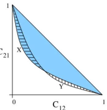
21 12 0 1 1 Y X C C
Figure 7. Illustration of the Gand δ measures forQ= 2. The shaded area denotes
G(X), the horizontally dashed area denotesδ(X, Y) and the vertically dashed area
denotesδ(Y, X).
of the unit hypercube dominated by this can be derived as follows: First we note that the volume of the pyramidal region between the origin and the sim-plex with vertices at a distance L along each coordinate vector is (QLQ(Q(Q−−1))!1) . The volume lying between the origin and the random allocation simplex is, therefore:
(Q−1)Q(Q−1)
(Q(Q−1))! . (14)
Only part of this volume lies in the unit hypercube however, as the corners (excluding that at the origin) relate to infeasible regions where classification rates are>1. Each of theseQ(Q−1) corner regions is also a pyramidal volume, but with sides of length Q−2. The total volume of the region between the origin and the random allocation simplex whichalso lies in the unit hypercube is therefore
(Q−1)Q(Q−1)
(Q(Q−1))! −
Q(Q−1)(Q−2)Q(Q−1)
(Q(Q−1))! . (15)
We denote this region byP. WhenQ= 2 the second term in equation 15 is zero so that the total volume (area) between the origin and the random allocation simplex is just 1/2. This corresponds to the area under the diagonal in a conventional ROC plot (although binary ROC plots are usually made in terms of true positive rates versus false positive rates for one class, the false positive rate for the other class is just 1 minus the true positive rate for the other class). However, when Q > 2, the volume not dominated by the random allocation simplex is very small; even whenQ= 3,the volume not dominated is≈0.0806. We therefore define G(X) to be the analogue of the Gini coefficient in two dimensions, namely the proportion of the volume of theQ(Q−1)-dimensional unit hypercube that is dominated by elements of the ROC surface, but is not dominated by the simplex defined by random allocation (as illustrated by the blue shaded area in Figure 7 for the Q = 2 case). In binary classification problems this corresponds to twice the area between the ROC curve and the
−0.80 −0.6 −0.4 −0.2 0 50 100 150 200 250 300
Signed distance from simplex
Number −0.80 −0.6 −0.4 −0.2 0 0.2 50 100 150 200 250 300
Signed distance from simplex
Number
G(k-nn) 0.916
G(MLP) 0.970
δ(k-nn,MLP) 0.0001
δ(MLP, k-nn) 0.054
Figure 8. Distances from the random classifier simplex. Negative distances
corre-spond to models inP.Left: k-nn;Middle:MLP.Right:Generalised Gini coefficients
and exclusively dominated volume comparisons of the k-nn and MLP classifiers.
diagonal. In multi-class problemsG(X) quantifies how much betterX is than random allocation. It can be simply estimated by Monte Carlo sampling ofP
in the unit hypercube.
If every point on the optimal ROC surface for classifier X is dominated by a point on the ROC surface for classifier Y, then classifier Y has a superior performance to classifier X. In general, however, neither ROC surface will completely dominate the other: regions of X’s surface,RX, will be dominated
by regions of Y’s and vice versa; in binary problems this corresponds to ROC curves that cross. To quantify the classifier’s relative performance we therefore define δ(X, Y) to be the volume of P that is dominated by elements of RX
and not by elements of RY (marked in Figure 7 with horizontal lines). Note
that δ(X, Y) is not a metric because although it is non-negative it is not symmetric. Also ifRX and RY are subsets of the same non-dominated set W,
(i.e., RX ⊆W and RY ⊆W), then δ(X, Y) and δ(Y, X) may have a range of
values depending on their precise composition; see Fieldsend et al. [2003] for more details. Situations like this are rare in practice, however, and measures like δ have proved useful for comparing Pareto fronts.
The right panel of Figure 8 shows G and δ calculated from 105 Monte Carlo
samples for the k-nn and MLP classifiers. The MLP ROC surface dominates a larger proportion of the volume and, as the δ measures show, almost every point on the k-nn ROC surface is weakly dominated by a point on the MLP surface. As mentioned above, the MLP has 33 adjustable parameters compared with 2 for k-nn, so it is unsurprising that the MLP front almost completely dominates the k-nn front.
It should be noted that not all of the classifiers located by the evolutionary algorithm lie in the volume P. This occurs because in multi-class problems, performance on one misclassification rate may be sacrificed to be worse than random in order to obtain superior performance on the other rates. In fact all of thek-nn models and all but 4 of≈4800 MLP models on the ROC surface lie in
P. Figure 8 shows histograms of the signed distances of classifiers on the ROC surface from the random allocation simplex; negative distances correspond to
classifiers in P. Clearly the majority of classifiers lie some distance closer to the origin than the random allocation simplex. In the absence of additional information or preferences (such as a maximum misclassification rate that can be tolerated for a particular class), a method of selecting the optimal classifier is to choose the one most distant from the random allocation simplex, a practice that corresponds to the selecting the classifier most distant from the diagonal on binary ROC plots.
6 Conclusion
In this paper we have considered multi-class generalisations of ROC analysis from a multi-objective optimisation perspective. Consideration of the role of costs in classification leads to a multi-objective optimisation problem in which misclassification rates are simultaneously optimised. The resulting trade-off surface generalises the binary classification ROC curve because on it one mis-classification rate cannot be improved without degrading at least one other. We have presented a straightforward general evolutionary algorithm which efficiently locates approximations to the Pareto optimal ROC surfaces. An appealing quality of the ROC curve is that it can be plotted in two sions and an operating point selected from the plot. Unfortunately, the dimen-sion of the Pareto optimal ROC surface grows as the square of the number of classes, which hampers visualisation. Projection into ‘false positive space’ is an effective visualisation method for 3-class problems as the false positive rates summarise the gross overall performance, allowing further analysis of exactly which classes are misclassified into which to be focused in particular regions. Nonetheless, it is likely that problems with more than three classes will require some a priori assessment of important trade-offs because of the difficulty in interpreting 16 or more competing rates. Reliable calculation and visualisation of the curvature of the ROC surface will be important for selecting operating points; current work is focused on this area.
The Pareto optimal ROC surface yields a natural way of comparing classifiers in terms of the volume that the classifiers’ ROC surfaces dominate. We defined and illustrated a generalisation of the Gini coefficient for multi-class problems that quantifies the superiority of a classifier to random allocation. Finally, we remark that some imprecise information about the costs of misclassification may often be available; for example the approximate bounds on the ratios of theλkj may be known. In this case the evolutionary algorithm is easily focused
on the relevant region by setting the Dirichlet parameters αkj appearing in (8) to be in the ratio of the expected costs, with their magnitudes setting the variance in the cost ratios.
References
N.M. Adams and D.J. Hand. Comparing classifiers when the misallocation costs are uncertain. Pattern Recognition, 32:1139–1147, 1999.
M. Anastasio, M. Kupinski, and R. Nishikawa. Optimization and FROC anal-ysis of rule-based detection schemes using a multiobjective approach. IEEE Transactions on Medical Imaging, 17:1089–1093, 1998.
C. Bishop.Neural Networks for Pattern Recognition. Clarendon Press, Oxford, 1995.
A.P. Bradley. The use of the area under the ROC curve in the evaluation of machine learning algorithms. Pattern Recognition, 30:1145–1159, 1997. C.A. Coello Coello. A Comprehensive Survey of Evolutionary-Based
Multiob-jective Optimization Techniques. Knowledge and Information Systems. An International Journal, 1(3):269–308, 1999.
T.M. Cover and P.E. Hart. Nearest neighbor pattern classification. IEEE Transactions on Information Theory, 13(1):21–27, 1967.
K. Deb. Multi-Objective Optimization Using Evolutionary Algorithms. Wiley, Chichester, 2001.
R.O. Duda and P.E. Hart. Pattern Classification and Scene Analysis. Wiley, New York, 1973.
R.M. Everson and J.E. Fieldsend. Multi-objective optimisation of safety re-lated systems: An application to short term conflict alert. IEEE Transac-tions on Evolutionary Computation, 2006. (In press).
J.Q. Fan and I. Gijbels.Local polynomial modelling and its applications. Chap-man & Hall, London, 1996.
J.E. Fieldsend and R.M. Everson. ROC Optimisation of Safety Related Sys-tems. In J. Hern´andez-Orallo, C. Ferri, N. Lachiche, and P. Flach, editors,
Proceedings of ROCAI 2004, part of the 16th European Conference on Ar-tificial Intelligence (ECAI), pages 37–44, 2004.
J.E. Fieldsend and R.M. Everson. Formulation and comparison of multi-class ROC surfaces. InProceedings of the 2nd ROC Analysis in Machine Learning Workshop, part of the 22nd International Conference on Machine Learning (ICML 2005), pages 41–48, 2005a.
J.E. Fieldsend and R.M. Everson. Visualisation of multi-class ROC surfaces. In Proceedings of the 2nd ROC Analysis in Machine Learning Workshop, part of the 22nd International Conference on Machine Learning (ICML 2005), pages 49–56, 2005b.
J.E. Fieldsend, R.M. Everson, and S. Singh. Using Unconstrained Elite Archives for Multi-Objective Optimisation. IEEE Transactions on Evo-lutionary Computation, 7(3):305–323, 2003.
P. Flach, H. Blockeel, C. Ferri, J. Hern´andez-Orallo, and J. Struyf. Decision support for data mining: Introduction to ROC analysis and its applications. In D. Mladenic, N. Lavrac, M. Bohanec, and S. Moyle, editors,Data Mining and Decision Support: Integration and Collaboration, pages 81–90. Kluwer, 2003.
D.J. Hand and R.J. Till. A simple generalisation of the area under the ROC curve for multiple class classification problems. Machine Learning, 45:171– 186, 2001.
J.A. Hanley and B.J. McNeil. The meaning and use of the area under a receiver operating characteristic (ROC) curve. Radiology, 82(143):29–36, 1982. J. Hern´andez-Orallo, C. Ferri, N. Lachiche, and P. Flach, editors. ROC
Anal-ysis in Artificial Intelligence, 1st International Workshop, ROCAI-2004, Valencia, Spain, 2004.
C.C. Holmes and N.M. Adams. A probabilistic nearest neighbour method for statistical pattern recognition. Journal Royal Statistical Society B, 64:1–12, 2002.
C.C. Holmes and N.M. Adams. Likelihood inference in nearest-neighbour classification models. Biometrika, 90(1):99–112, 2003.
J.D. Knowles and D. Corne. Approximating the Nondominated Front Using the Pareto Archived Evolution Strategy. Evolutionary Computation, 8(2): 149–172, 2000.
M.A. Kupinski and M.A. Anastasio. Multiobjective Genetic Optimization of Diagnostic Classifiers with Implications for Generating Receiver Operating Characterisitic Curves. IEEE Transactions on Medical Imaging, 18(8):675– 685, 1999.
D. Mossman. Three-way ROCs. Medical Decision Making, 19(1):78–89, 1999. F. Provost and T. Fawcett. Analysis and visualisation of classifier performance: Comparison under imprecise class and cost distributions. In Proceedings of the Third International Conference on Knowledge Discovery and Data Mining, pages 43–48, Menlo Park, CA, 1997. AAAI Press.
F. Provost and T. Fawcett. Robust classification systems for imprecise envi-ronments. In Proceedings of the Fifteenth National Conference on Artificial Intelligence, pages 706–7, Madison, WI, 1998. AAAI Press.
B.D. Ripley. Neural networks and related methods for classification (with discussion). Journal of the Royal Statistical Society Series B, 56(3):409– 456, 1994.
M.J.J. Scott, M. Niranjan, and R.W. Prager. Parcel: feature subset selection in variable cost domains. Technical Report CUED/F-INFENG/TR.323, Cambridge University Engineering Department, 1998.
A. Srinivasan. Note on the location of optimal classifiers in n-dimensional ROC space. Technical Report PRG-TR-2-99, Oxford University Computing Laboratory, Oxford, 1999.
D. Van Veldhuizen and G. Lamont. Multiobjective Evolutionary Algorithms: Analyzing the State-of-the-Art. Evolutionary Computation, 8(2):125–147, 2000.
X. Yao, Y. Liu, and G. Lin. Evolutionary Programming Made Faster. IEEE Transactions on Evolutionary Computation, 3(2):82–102, 1999.
M.H. Zweig and G. Campbell. Receiver-operating characteristic (ROC) plots: a fundamental evaluation tool in clinical medicine. Clinical Chemistry, 39: 561–577, 1993.