Interactive Simulation of Clouds Based on Fluid Dynamics. Diplomarbeit

(1)

Fachbereich 4: Informatik

Interactive Simulation of Clouds

Based on Fluid Dynamics

Diplomarbeit

zur Erlangung des Grades eines Diplom-Informatikers im Studiengang Computervisualistik

vorgelegt von

Oliver Koehler

Erstgutachter: Prof. Dr.-Ing. Stefan Müller

(Institut für Computervisualistik, AG Computergraphik) Zweitgutachter:

(2)

Erklärung

Ich versichere, dass ich die vorliegende Arbeit selbständig verfasst und kei-ne anderen als die angegebekei-nen Quellen und Hilfsmittel benutzt habe.

Ja Nein Mit der Einstellung der Arbeit in die Bibliothek bin ich einverstanden. Der Veröffentlichung dieser Arbeit im Internet stimme ich zu.

. . . .

(3)

List of Figures

1 Fractal Sphere created with a noise function, image courtesy of Perlin [17] . . . 4 2 Cumulus (left) and cirrostratus clouds (right) rendered with

Ebert’s method, images courtesy of Ebert [3] . . . 5 3 Cumulus clouds rendered with Schpok’s GPU-assisted method,

images courtesy of Schpok [19] . . . 5 4 A cloudscape combining 2D- and 3D-clouds by Gardner,

im-age courtesy of Gardner [7] . . . 6 5 Noise textures as used by Gardner (left) and Elinas/Stuerzlinger

(right), courtesy of Elinas/Stuerzlinger [4] . . . 7 6 Real-time static clouds created by Lastra et al., image taken

from [13] . . . 7 7 A screen shot from Foster & Metaxas work on fluid

simula-tion, image courtesy of Foster & Metaxas [6] . . . 9 8 A cloud and smoke simulated with Stam’s method, images

courtesy of Stam [20] . . . 9 9 A picture from Fedkiw’s smoke simulation that preserves

small scale details, images courtesy of Fedkiw et al. [5] . . . 10 10 Image computed with Kajiya’s method, courtesy of Kajiya/von

Herzen [12] . . . 10 11 Cumulus (left) and stratus clouds (right) generated with Overby’s

method. The red dots in the left image represent heat and vapor sources. Image courtesy of Overby [16]. . . 11 12 Static, particle-based clouds rendered with Harris’ method,

courtesy of Harris [8] . . . 11 13 Binary values represent the state values in Dobashi’s method

based on cellular automatons. Image taken from [2] . . . 12 14 Clouds created by Dobashi et al., images taken from [15] . . 12 15 The dew point curve. It specifies the relation between dew

point (in red) and temperature, as well as the correspondent water vapor mixing ratios . . . 16 16 Stable and unstable atmospheric conditions. The black line

describes the temperature gradient of the atmosphere. . . 19 17 Cloud classification according to altitude, with official

abbre-viations and symbols . . . 20 18 Schematic view of a warmfront . . . 21 19 Schematic view of a cold front . . . 22 20 Use of the Nabla-operator in fluid dynamics, courtesy of Mark

Harris [8] . . . 25 21 The air pressure decreases exponentially with altitude,

(6)

22 Tracing a pseudo-particle backwards through the velocity field and interpolating between the surrounding cells(left), copying the interpolated value to the grid position (right) . . 36 23 The divergence-free velocity field (left) consists of a

diver-gent velocity field (middle) minus the pressure gradient field (right), courtesy of Stam [21] . . . 37 24 This image shows how the clouds are rendered (in 2D). The

red dots correspond to the centers of the grid cells. . . 42 25 The user interface . . . 44 26 Cumulus clouds developing under stable conditions, and

the corresponding velocity fields. Images were taken after 340 iterations (left) and 760 iterations (right). The bottom image shows the temperature distribution. . . 47 27 Cumulus clouds developing under unstable conditions, and

the corresponding velocity fields. Images were taken after 300 iterations (left) and 600 iterations (right). . . 48 28 Stratus clouds develop as humid air is blown in from the

(7)

1 Introduction

Humankind has always been fascinated by clouds. It seems amazing how these enormous and seemingly solid structures just float around in the sky and how they appear and disappear out of nothing. The work of count-less poets, authors and songwriters has been influenced by the observation of clouds and the phenomena associated with them. From the menacing atmosphere transmitted by an approaching thunderstorm to the colorful and soothing display of clouds at sunset, they can evoke a wide variety of emotions. Painters of all styles and epochs have tried to capture these spectacular scenes in their paintings.

Before today’s scientific weather forecast came to be, looking at the skies was the only possible way to get an indication of how the weather might be in the near future. In pre-industrialized, rural society, the ability to rec-ognize and interpret cloud patterns was of vital importance. Today, even though the understanding about cloud formations is not necessary for sur-vival anymore, it can still be useful to complement the official weather fore-cast with local details.

In the computer science community, and especially in computer graph-ics, a lot of research has been done in order to achieve realistic renditions of clouds, because they are an indispensable element of any outdoor scene. However, most cloud models developed did not simulate the actual phys-ical processes but took a more artistic approach, since a physphys-ically moti-vated simulation of clouds is computationally very expensive. Only re-cently has sufficient computational power become available to use physics-based cloud simulation in computer graphics. Still, certain assumptions have to be made and some concepts have to be simplified in order to keep frame rates at interactive levels.

The cloud model developed in this thesis attempts to correctly model the physical processes involved in cloud formation. It incorporates con-cepts from fluid dynamics and thermodynamics, and renders the results to the screen using techniques from computer graphics.

The goal is to achieve a simulation that runs at interactive frame rates and that allows the user to visually experience the basic processes involved in cloud formation. It should also be possible to interactively change im-portant parameters of the simulation and observe the consequences in near real-time. It was therefore necessary to develop visual representations of different aspects of the cloud simulation, such as the velocity or tempera-ture.

This thesis is organized as follows: Chapter 2 introduces the most im-portant works and approaches for the modeling and rendering of clouds. Both procedural and physics based approaches are presented.

In chapter 3, the most important quantities and mechanisms involved in cloud formation in the atmosphere are presented in a comprehensible

(8)

manner, while chapter 4 puts these principles on a more formal basis. It describes the models and equations used in the cloud model, based on at-mospheric physics, and also explains where and why certain aspects were simplified. Chapter 5 then describes how the aforementioned equations and concepts are solved on the computer. It also sheds some light on the rendering method that has been employed, as well as explaining the vi-sual helps that were developed for the vivi-sualization of the cloud dynamics. The results are presented in chapter 6, also discussing the limitations and shortcomings of the proposed cloud model and simulation method.

(9)

2 Related Works

Clouds are omnipresent in any outdoor scene and it therefore comes as no surprise that a lot of research has been done with the aim of creating re-alistically looking clouds. Many of these techniques are not intended for a physically accurate simulation but rather focus on the visual aspects of clouds. However, in order to achieve an exhaustive description of previous works related to the problem at hand, the following section will provide an overview over most of the techniques that have been used for the simula-tion and rendering of clouds.

When simulating clouds, two distinct fields of research have to be taken into account. First, there is the simulation of the physical processes that govern the formation of clouds. These processes can be described by the laws of atmospheric fluid dynamics. While these laws have been known in meteorology for quite some time, only lately (e.g. Since the end of the 1990s) do consumer class workstations dispose of sufficient computational power to perform the required calculations at interactive rates. Especially the advent of programmable graphics processors (GPUs) has fueled this development, since they are designed for parallel execution of several cal-culations at once.

The second important aspect of cloud simulation is rendering. A cloud dynamics simulation typically delivers a three-dimensional density distri-bution, and therefore requires a method to render this volumetric data.

2.1 Cloud Modeling

The modeling of clouds is a challenge for every developer due to their amorphous nature. Since they constantly appear, disappear, and change shape, clouds cannot easily be modeled using solid geometric primitives, although such approaches do exist. The distinction that is taken here in or-der to classify different cloud modeling techniques differentiates between procedural approaches and physically motivated techniques. While the first tackle the problem more from an artist’s perspective and focus on visually convincing cloud modeling and rendering techniques, physically motivated approaches try to capture and simulate the underlying physical processes that are responsible for the formation of clouds. It should how-ever be noted, that the different techniques presented here are by no means mutually exclusive. In fact, most works use a combination of several meth-ods.

2.1.1 Procedural Techniques

Throughout the history of computer graphics, procedural approaches have been very popular for the modeling of natural phenomena such as clouds,

(10)

fire, smoke, or for the creation of textures that are intended to resemble natural materials like marble, wood, or stone. Procedural techniques use algorithms to specify the properties of the desired materials (for exam-ple its color or opacity value), and therefore don’t rely on photographs or handmade images as input. This reduces memory requirements and elimi-nates the need to have an artist manually design these models and textures. Another advantage of procedural techniques is that they usually specify a number of parameters (such as a value for the ’roughness’ of a mate-rial) that offer an increased level of flexibility to the animator/modeler [3]. In fact, most professional animating software suites (like Maya or 3D Stu-dio Max) offer some procedural methods to model natural phenomena like smoke or fire.

Noise One procedural technique that has been used in several works in cloud modeling is procedural noise. Noise is an adequate method for mod-eling seemingly “chaotic” phenomena like clouds or smoke, and it is also useful to represent the irregularities that many natural materials like stone or wood typically exhibit. It can also be employed to give materials a more “rugged” or “used” look.

In 1989, Ken Perlin [17] presented a method to create continuous ran-dom volumetric data based on procedural noise, which is applicable not only to clouds, but to a wide array of materials. His methods extends the idea of procedural solid textures to three dimensions. Clouds are modeled as density fields that are then modulated by the sum of a series of pseudo-random noise functions at different amplitudes and frequencies [17]. Fig-ure 1 shows a sphere that has been contorted with a fractal sum of noise functions.

Figure 1:Fractal Sphere created with a noise function, image courtesy of Perlin [17]

In 2004 Ebert presented an approach to modeling clouds that also re-lies on noise and turbulence [3]. He models the cloud macro structure as

(11)

a union of implicit geometric primitives like spheres, cylinders, or ellip-soids. These are placed by the user, who thus directly influences the basic shape of the clouds to be. Comparable to Perlin, the macro structure of the clouds is then perturbed by procedural noise and turbulence functions that account for the small-scale details, the cloud’s micro structure. Depending on the primitives used for the cloud’s macro structure and several param-eters like thickness, falloff, or density, different cloud types can be created. Coupled with a physically based volume renderer that accounts for the ef-fects of light scattering, very realistic images and animations of clouds can be achieved, however not in real time. Figure 2 shows two examples of different cloud types.

Figure 2:Cumulus (left) and cirrostratus clouds (right) rendered with Ebert’s method, images courtesy of Ebert [3]

Building on Ebert’s work and using the same two-level approach, Sch-pok et al. [19] extended the technique to draw on the additional comput-ing power available through consumer graphics hardware. By reallocatcomput-ing computationally expensive tasks to the graphics processor and using a less refined illumination model, they were able to reach interactive frame rates, between 5 and 30 fps [19]. See figure 3 for examples.

Figure 3:Cumulus clouds rendered with Schpok’s GPU-assisted method, images courtesy of Schpok [19]

(12)

Textured Solids One significant disadvantage of volumetric cloud repre-sentations is their computational complexity. Especially in real-time appli-cations such as flight simulators, fast modeling and rendering techniques are indispensable. There have been several attempts to model clouds as textured solids, because this representation promises the best performance. One early work following this approach was presented by Geoffrey Gardner in 1985 [7]. His cloud model consists of three building blocks: A two-dimensional sky plane is used to represent layer clouds and serves as a backdrop. In this way, clouds that are further away are not explicitly modeled in 3D, thus increasing performance. The macro structure of cu-mulus clouds and other cloud types that cannot be adequately modeled in two dimensions because they are relatively close to the camera, consists of ellipsoids. In order to allow for more complex cloud shapes, several ellip-soids can be linked together. Similar to Ebert [3], noise textures are used to modulate the shading intensity and translucency. Given that his work was published almost 25 years ago, the results (see figure 4) are quite im-pressive, although it has to be noted that at the time, rendering of a single image took between 20 and 25 minutes [7].

Figure 4:A cloudscape combining 2D- and 3D-clouds by Gardner, image courtesy of Gardner [7]

Based on Gardner’s work, Elinas and Stuerzlinger [4] extended this ap-proach in 2000 to make use of new technological advances like photon maps using hardware-accelerated OpenGl. They also changed the way their textures are created: While Gardner relied on spectral synthesis, they used Perlin noise to create the textures that regulate transparency and color. Figure 5 shows a comparison between different noise textures.

Particle Systems Another cloud modeling technique is based on parti-cles. Particles are small geometric primitives (often spheres) that can be de-scribed by their position in three-dimensional space and only a few other

(13)

Figure 5:Noise textures as used by Gardner (left) and Elinas/Stuerzlinger (right), courtesy of Elinas/Stuerzlinger [4]

parameters (like radius, color, texture, etc.) [8]. As such, they are relatively easy to implement and inexpensive to manage, and are therefore often used in real-time applications. Many systems that model gaseous phenomena like smoke, fire or clouds rely on particle systems, since they can be used in conjunction with an underlying physics engine. However, the advantage of using particle systems diminishes somewhat when a lot of small-scale details are required, because the number of particles has to be increased considerably.

Lastra and Harris [13] presented their cloud modeling approach in 2001. They represent clouds as a collection of particles and render each particle as a small, textured sprite. Building on a technique introduced by Gardner [7], they introduced the use of impostors, 2D-textures that represent clouds that are farther away. Since only near clouds are modeled in 3D, they achieved very high frame rates. However, their method could only represent static clouds and did not involve any sort physical model.

(14)

2.1.2 Physics-Based Cloud Simulation

The procedural approaches to cloud modeling presented so far are aimed mostly at achieving visually convincing representations of clouds, and are less concerned with the underlying physics. In fact, from an artist’s point of view, a procedural approach is preferable because it offers more control over the shape and appearance of the clouds.

Physics-based cloud modeling takes a different approach. The goal here is to accurately portray the physical processes that are responsible for the formation of clouds in nature. The clouds that are modeled in this fashion should come into being as the result of applying the laws of nature and physics, combined with techniques from computer graphics to render the results. As such, an animator has only indirect control over the process, because he can typically only specify certain parameters that correspond to real physical quantities and then has to “let nature do the rest”.

Fluid Dynamics Physics-based cloud dynamics are closely linked with fluid dynamics, because the laws from fluid dynamics (namely the Navier-Stokes equations) can be used to accurately describe the flow of air masses in the atmosphere. All approaches to modeling the dynamics of clouds im-plement some method to solve these equations. Since fluid dynamics and the Navier-Stokes equations play such an integral part in the simulation of clouds, some works that were important in the development of fluid solvers are presented first, although these works are generally not focused on clouds, but comparable phenomena such as smoke, fire, or liquids.

The Navier-Stokes equations have been known for more than a hun-dred years. They model fluid flow using a set of non-linear partial dif-ferential equations in terms of velocity and pressure (see chapter 4 for an in-depth explanation). In 1995, Foster and Metaxas [6] described a incre-mental method to numerically solve these equations. Their approach was based on a rectangular grid that divides space into voxels, and the Navier-Stokes equations were solved incrementally for each voxel. The problem with this approach was that it suffered from instability when the time step for the simulation became too large. Allowing only small time steps how-ever, increases computation time.

Based on the work of Foster and Metaxas, Stam developed a method that guaranteed unconditional stability for any time step size [20][21]. In-stead of the previous explicit time stepping scheme, he used an implicit, semi-Lagrangian method that borrowed ideas from particle systems. To-day, many works in computer graphics that try to simulate some kind of fluid flow are based on Stam’s method, and it has also been used in this thesis (see chapter 5).

The most important drawback of Stam’s method is that it leads to dis-sipation, thus damping out some of the small-scale swirls and turbulences

(15)

Figure 7:A screen shot from Foster & Metaxas work on fluid simulation, image courtesy of Foster & Metaxas [6]

Figure 8:A cloud and smoke simulated with Stam’s method, images courtesy of Stam [20]

typically encountered in fluid motion. Fedkiw et al. approached this prob-lem in [5], introducing a method called “vorticity confinement” that rein-troduces lost rotational energy back into the fluid. This method allows more detailed fluid flows.

Cloud Dynamics The first physics based models of cloud dynamics were developed by meteorologists and atmospheric scientists. As they were used only as scientific tools, they were focused on accurately modeling the physical processes, and less on performance and rendering. The enormous computational complexity involved in simulating cloud dynamics further hindered the application of physically motivated cloud models to any other domain but meteorology and atmospheric sciences.

The first in developing a physically based cloud model for computer graphics were Kajiya and von Herzen in 1984 [12]. They solved the Navier-Stokes equations of incompressible fluid flow and also incorporated a ther-modynamics model and a simple water continuity model [16]. With their method they achieved solving one step of cloud evolution in about 10 sec-onds on a 10x10x20 grid.

A similar method was presented by Overby in 2002 [16]. In this work, the stable fluid simulation algorithm developed by Stam [20] was used to

(16)

Figure 9:A picture from Fedkiw’s smoke simulation that preserves small scale details, images courtesy of Fedkiw et al. [5]

Figure 10:Image computed with Kajiya’s method, courtesy of Kajiya/von Herzen [12]

solve the Navier-Stokes equations. Overby modeled the water in the sys-tem in terms of relative humidity, with saturation values directly propor-tional to pressure. The model also accounted for the existence of cloud con-densation nuclei, small particles in the air that have can lower or raise the saturation threshold. The user interface allowed to create different cloud types (cumulus, stratus) by changing the initial conditions of the simula-tion.

The volumetric data resulting from the simulation was then rendered using alpha-blended billboards, thus achieving a performance of one itera-tion per second on a Pentium III with a 15x50x15 grid [16].

The work presented by Mark Harris in 2003 [8] was the first that achieved frame rates fit for real-time applications by consequently exploiting the

(17)

Figure 11:Cumulus (left) and stratus clouds (right) generated with Overby’s method. The red dots in the left image represent heat and vapor sources. Image courtesy of Overby [16].

computational power of graphics hardware. He developed a fairly com-plicated cloud model and used Stam’s stable fluid algorithm [20] for the dynamics, and implemented both on the GPU. In order to further enhance performance, a technique called “simulation amortization” was developed that spreads the dynamics calculations over several frames.

For the rendering of the clouds, algorithms were developed that simu-late multiple forward light scattering, and that are applicable both to parti-cle and voxel based cloud representations. In order to speed up the render-ing process, dynamically generated impostors were used. These are basi-cally two-dimensional textures that can be applied to represent clouds that are so far away from the camera that they do not have to be represented in 3D. Similar techniques had already been described in [7], [22], and [13].

Harris cloud simulation achieved frame rates of up to 3.9 frames per second on a 64x64x64 grid and using GeForce 5900 Ultra in conjunction with a Pentium IV CPU.

Figure 12:Static, particle-based clouds rendered with Harris’ method, courtesy of Harris [8]

(18)

experi-mented with simpler (and therefore faster) approximations of fluid flow. in 2000, Dobashi et al. [2] presented a method that approximates the behavior of clouds with cellular automatons. This method models cloud evolution on a voxel grid, just like the other physics-based approaches. The state values however are represented as logical (binary) values that change according to logical transition rules that simulate evaporation, con-densation, etc. While this method is very fast, it is not able to simulate the processes of cloud formation accurately (see figure 13).

Figure 13:Binary values represent the state values in Dobashi’s method based on cellular automatons. Image taken from [2]

Figure 14:Clouds created by Dobashi et al., images taken from [15] An extension of this method was presented by Myiazaki et al. in 2001 [15]. The basic idea was to use a concept called “coupled map lattices” (CML) instead of the cellular automatons, because they allow to use contin-uous instead of only binary values. The transition rules were than replaced by an approximation of the incompressible Navier-Stokes equations. The model presented in 2001 [15] was able to depict different cloud types, while another work presented in 2002 [14] explored more accurate ways to model cumulus clouds. Both these models included a water continuity model and also accounted for latent heat release due to phase changes.

All these works used volume rendering techniques using metaballs and splatting. Their rendering also included a lighting model and could depict shafts of light in between clouds. However, this rendering technique,

(19)

al-though producing very convincing images, is not suited for real-time ap-plications.

2.2 Rendering Techniques for Volumetric Data

Virtually all works that realize a simulation of clouds based on the laws of atmospheric physics (or an approximation of them) model clouds on a voxel grid. Using this technique, the results of the simulation are provided in the form of a three-dimensional distribution of state values. Therefore they all require some volume rendering technique to visualize the results.

One possible method to render this data is ray tracing. However, since the goal of this thesis is to achieve interactive frame rates, ray tracing is not an option because it is too computationally expensive. The same is true for the metaball splatting technique developed by Dobashi et al. [2].

The method used in this thesis renders alpha-blended slice from front to back.

2.3 Summary

There is a multitude of different approaches available to render and sim-ulate clouds. However, the selection of works presented here also reflects the eternal dilemma of computer graphics, to choose between quality and performance. Since the stated goal of this thesis is to achieve interactive frame rates while as accurately as possible simulating the physics of cloud formation, only few works could be used as orientation.

The cloud model developed in this thesis is most similar to those pre-sented by Overby [16] and Harris [8]. Both model the physical processes involved in cloud dynamics. While this thesis uses the more accurate dy-namics model presented by Harris, it was also influenced by the idea of simulating different cloud types introduced by Overby. Since the focus in this work lies more on depicting and visualizing the physical processes in-stead of achieving visually realistic results, a much simpler cloud rendering method was chosen for the sake of performance (presented in chapter 5.2).

(20)

3 Cloud Formation in the Atmosphere

The following chapter serves as an introduction to the formation of clouds. It focuses on the description of the most important concepts involved in the formation of clouds, and it is designed to be as comprehensible as possible. The ideas presented here will then be put on a more theoretical foundation in chapter 4.

3.1 Air Parcels

In order to better understand the processes involved in cloud formation, it is common in meteorology to study the behavior of air parcels. Such an air parcel is a conceptual tool that can be imagined as a thermically iso-lated volume of air that is able to expand and contract without any exterior force, and that can be traced relative to its surroundings. Although this idea might at first seem unrealistic, it actually matches the behavior real volumes of air quite well[9], because air has very low thermal conductivity.

3.2 Water and Humidity

Water is the most important property in climatology and meteorology. It occurs in all three physical states: as gas in the form of vapor, as a liquid in the form of water and water droplets, and in its solid state in the form of ice and snow. The weather on our planet and especially the formation of clouds rely heavily on the state changes that water undergoes in the atmo-sphere due to changing temperature and/or pressure. On a global scale, it is water and air currents that are responsible for the climatic conditions on our planet. For example, the gulf stream, a warm water current that originates in the gulf of Mexico and extends all the way to western Europe, is responsible for the moderate climate we enjoy in central and northern Europe.

The air on our planet always contains some amount of water vapor that comes into being through the process of evaporation. The majority of evap-oration occurs over the oceans and other open waters such as lakes and rivers, but a certain part is also due to transpiration of plants, humans, and animals, as well as evaporation of ground water. It is estimated that the total amount of water present on earth is about 1,4 billion km. Of this total amount, less than 0,001%, or 13000 km is contained in the atmosphere as humidity and clouds [9]. Although it is but a tiny fracture, this atmospheric water is completely responsible for the formation of the clouds all over the world. It is generally referred to as humidity. There are several commonly used quantities that describe the relationship between air and vapor:

(21)

Absolute Humidity It describes the absolute amount of water vapor that is contained in a specific volume of air. It is usually specified in grams per cubic meter, but different units, such as pounds per cubic foot, are also commonly used in different parts of the world. The major inconvenience with this quantity is that it it is only constant for a certain altitude. When an air parcel changes its altitude, its volume also changes due to different pressure conditions. As a consequence, the absolute humidity changes as well.

Specific Humidity This quantity specifies the humidity in grams of water vapor per kg of air. By using mass instead of volume, specific humidity stays constant regardless of altitude and pressure. It is therefore much more commonly used. In the cloud model developed for this thesis, humidity is specified in this fashion. It is also often referred to as “water vapor mixing ratio”.

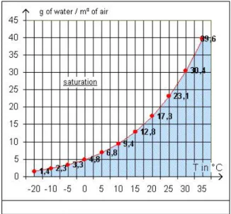
Relative Humidity The maximum amount of water vapor that air can contain depends directly on its temperature. Warm air can contain much more vapor than cold air. Relative humidity is calculated as the quotient between the specific humidity and the maximum amount of vapor possible, and it is usually expressed as a percentage. In other words, it expresses to what percentage the air is saturated with vapor. This quantity is very useful in weather forecast, as a high relative humidity increases the likelihood of precipitation. On the other hand, it can be difficult to work with due to its direct dependence on temperature. An indication of temperature is therefore required in order to give the relative humidity any meaning. Dew Point Another quantity that is closely related to humidity and that is needed in order to understand and calculate the relative humidity is the dew point. As mentioned above, the maximum amount of vapor that can be contained in the air depends on its temperature. When an air parcel with a given specific humidity cools down, its relative humidity rises. Eventu-ally, the relative humidity will reach 100% and the air is thus fully satu-rated with vapor. This point is called the dew point. Figure 15 shows the so-called dew point curve (at sea level) that indicates how many grams of water vapor can be contained in a kg of air at a given temperature.

Given these quantities it is now possible to describe the basic physical process, that leads to the formation of clouds. Once a parcel of air passes 100% relative humidity/its dew point/its saturation point, some of the va-por contained in it has to be expelled. At this point, condensation sets in. A certain part of the water in the air changes its physical state from gaseous to liquid and tiny water droplets begin to form. These droplets then be-come visible as clouds and fog. The exact amount of vapor that changes its

(22)

physical state to water is such that the surrounding air always stays 100% saturated. The question then is, what circumstances are responsible for air to become saturated with vapor and therefore form clouds? The answer to this question can be obtained by again looking at the dew point curve in figure 15. As the diagram shows, cool air can hold much less vapor before being saturated than warm air. Therefore, in order for clouds to form, air has to cool beyond the dew point associated with the amount of vapor that it holds.

Figure 15:The dew point curve. It specifies the relation between dew point (in red) and temperature, as well as the correspondent water vapor mixing ratios

3.3 Pressure and Temperature

There are several processes that can cause a change in the temperature of air parcels. For the formation of clouds, the most important process consists in a change of altitude. As is common knowledge, air temperature decreases with increasing altitude. This is due to the decrease of air pressure.

The air pressure experienced at a certain point corresponds, roughly, to the weight of the column of air above said point, multiplied by gravity. This explains why the air pressure decreases with height. Since at higher altitudes there is less air weighing down on it, the pressure at the point is less than in lower altitudes. An important property of air is that it is a compressible gas. Its volume thus changes according to different pres-sure conditions. This change in volume is also responsible for the change in temperature. Between the air molecules exists a force that draws them together. When the air expands, energy is required to overcome this force.

(23)

This energy is taken from the latent energy of the air, stored as heat. The air therefore cools as it expands. When it is compressed, the process is re-versed. The same principle is used, for example, in diesel engines, where the mixture of air and fuel is compressed heavily until it explodes.

3.4 Atmospheric Stability

We now know why rising air parcels tend to cool, thus causing condensa-tion. However, in order to simulate the cloud formation process, it has to be known at what rate rising air parcels cool down. As a rule of thumb, air cools at a rate of just about 1◦C per 100 meters as long as it is not saturated. In thermodynamics, this is referred to as “dry adiabatic cooling”, and it can be considered somewhat of a “standard behavior” [9].

When an air parcel is saturated (e.g. its relative humidity passes 100%), some of the vapor condensates. During the process of condensation, latent energy is released in the form of heat, thus warming the air parcel. This can be explained as follows: The evaporation of water (the change from liquid to gaseous form) requires energy (usually from the sun in the form of heat). This energy remains “stored” in the vapor as latent energy. When the vapor condensates this latent energy is released again as heat. As a con-sequence of the release of latent heat during condensation, the cooling rate of a saturated air parcel is lower than an unsaturated one. This is refered to as “wet adiabatic cooling”. The wet adiabatic cooling rate however, is not constant, since it depends on the amount of vapor that condensates and on the temperature. An average value is 0.6◦C per 100 meters.

If and how far an air parcel rises does not only depend on its own tem-perature but mostly on the temtem-perature of the air that surrounds it. If the surrounding air is cooler, an air parcel will rise, if it is warmer, it will de-scend. Therefore the temperature distribution of the atmosphere plays an essential role in the cloud formation process.

The Earth’s atmosphere is divided into several layers. Clouds can only form in the bottom layer, the troposphere (with a few rare exceptions). It is limited at the top by the tropopause, an imaginary line that also marks the beginning of the ozone layer. As the ozone layer absorbs energy in the form of ultraviolet radiation, the air temperature begins to rise again, thus forming an impassable barrier for air parcels coming from below. Therefore no clouds can form above the tropopause.

3.4.1 Stable Atmosphere

In the troposphere the temperature distribution can differ quite consider-ably from the adiabatic ideal. A temperature drop of less than 1◦C per 100 meters is referred to as underadiabatic. This is very often the case. In fact, the International Standard Atmosphere (ISA), a standardized atmospheric

(24)

model of the Earth’s atmosphere, shows only a temperature lapse of 0.65◦ C per 100 meters. This figure can be thought of as a general average. Espe-cially in the winter it is even possible that the temperature increases with altitude, at least for a certain part of the troposphere. This phenomenon is called an inversion.

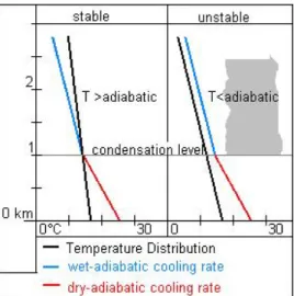
As a consequence of under adiabatic stratification, the troposphere be-comes very stable, since it impedes vertical air movements. The left hand side of figure 16 demonstrates this: When an air parcel is lifted to a given altitude, it cools adiabatically. However, since the surrounding atmosphere shows an underadiabatic temperature gradient, it cools slower than the air parcel and the air at the new altitude will be warmer. As a consequence, the air parcel will not rise further and even move downwards until it reaches its original altitude where its temperature is the same as the surrounding air. Since there are therefore only very few vertical air movements, the atmosphere and the weather become very stable. As far as clouds are con-cerned, a stable atmosphere manifests itself in stratus or cirrus clouds (the next section explains the different cloud types in more detail) that have only a limited vertical extension [9].

3.4.2 Unstable Atmosphere

The atmosphere can also exhibit an overadiabatic temperature gradient. This means that the temperature drops faster than adiabatically with in-creasing altitude. The result is contrary to the aforementioned case of a stable atmosphere: instead of hindering vertical air movements and tur-bulence, an overadiabatic temperature gradient even increases them, thus leading to an unstable atmosphere. This is shown on the right side in fig-ure 16. Such unstable conditions often occur in hot and humid climates. In our moderate climate zone this mostly happens in the summer: As the sun heats the ground, the air directly above it is also heated and starts to rise. As this process continues, the atmosphere becomes increasingly unstable as the temperature gradient between lower and higher altitudes grows. Since the unstable atmosphere furthers the rise of heated air parcels, clouds with a large vertical extension, like cumulus or even nimbocumulus develop that often lead to heavy rainfall and even thunderstorms.

It has to be noted that the temperature gradient of the troposphere is generally not constant. The atmosphere may be unstable at low altitudes and exhibit stable conditions further up, all at the same time. Several cloud layers of different cloud types are often a sign that the stability conditions vary at different altitudes. In general, the lower layers of the atmosphere are the most susceptible to becoming unstable because the ground, heated by the sun, can drastically change the temperature gradient.

(25)

Figure 16:Stable and unstable atmospheric conditions. The black line describes the temperature gradient of the atmosphere.

3.5 Cloud Classification

When one glances at the sky and observes the myriad of different shapes and appearances of clouds, it seems at first almost impossible to consis-tently categorize them. From puffy summer clouds that resemble cotton candy, to the gray-in-gray that seems to cover the entire sky on a dull winter day, from dark, menacing thunderstorms to light, translucent high-altitude clouds, the dazzling array of shapes and sizes that clouds exhibit seems limitless.

The classification that is used today dates back to the beginning of the 19th century [10]. Today, it is managed and constantly updated by the World Meteorological Organization(WMO), a sub-organization of the United Nations. The International Cloud Atlas, published by the WMO, serves as an international guideline for the classification and description of clouds observed all over the world [10].

3.5.1 Classification according to WMO

In general, there are ten different types of clouds, although these types can be further classified according to their shape.

The first criterion to distinguish different categories of clouds is the al-titude in which they appear. Since clouds can exist in all alal-titudes up to the tropopause, the distinction between different cloud families is made according to the physical state of the water they consist of. High altitude clouds are called “Cirrus” (from the Latin word for hair locks) and they consist only of ice crystals. In moderate climate zones, they can appear at altitudes between 5 and 13 km.

(26)

Medium altitude clouds have the prefix “Alto-” (lat. Altus = high). They can show up between 2-7 km above the ground and contain ice crys-tals as well as water droplets.

Low altitude clouds can be found from the ground up to altitudes of about 2 km. They are designated with the word “Stratus” and they consist only of water droplets.

A fourth category is that of clouds which exhibit a strong vertical ex-tension. These clouds can span more than ten kilometers in height and are not limited to a certain altitude. One example for this cloud type are the impressive cumulonimbus, or thunderstorm clouds.

The second criterion in this classification refers to the general shape of the clouds. Cumulus clouds are heap-shaped, while stratus clouds form a more or less uniform layer. The final designation for a certain cloud type is then a combination of these criteria: stratocumulus are low, heap-shaped clouds consisting of condensed water, cirrostratus are a uniform layer of high-altitude ice crystal clouds. The different cloud types are shown in figure 17.

Figure 17:Cloud classification according to altitude, with official abbreviations and symbols

3.5.2 Classification according to formation process

Since we are trying to simulate the formation of clouds, it is more use-ful to categorize clouds according to the processes that are responsible for their existence. In general, clouds form due to vertical air movements. The

(27)

causes for these movements differ, however.

Convective clouds form as a consequence of the heating of surface air. This happens when the sun heats the ground. Parcels of heated air then start to form over the heated surface and subsequently begin to rise. Their upward velocity can be quite high, reaching up to 30m/s under very un-stable conditions [9]. Once they reach higher altitudes, the vapor contained in them starts to condensate and form clouds. The condensation process releases latent heat, thus warming the parcel even further and fueling its ascension. This is the reason why cumulus clouds always grow upwards. If the atmospheric conditions are right, e.g. if the atmosphere is unsta-ble and the ground temperature is high enough, as is often the case in the summer, cumulus clouds can keep growing upwards, eventually forming cumulonimbus clouds that can bring strong precipitations, violent gusts of wind and thunderstorms.

Another important mechanism for cloud formation is the general tem-perature change caused by incoming cold or warm fronts. A warm front ar-rives first in high altitudes because the warm air glides on top of the colder air masses. The warm front gradually pushes away the colder air, until the warm air masses reach the ground. In profile, an approaching warm front takes on the form of a wedge (see figure 18). As a consequence of the warm air being lifted, an incoming warmfront usually reveals itself by an increasing number of cirrus clouds. As time passes and the warm air grad-ually replaces the cold air, the cloud layer eventgrad-ually becomes thicker and grows downwards, transforming into Cirrostratus, Altostratus, and finally Nimbostratus, that can bring abundant and long lasting rainfalls.

Figure 18:Schematic view of a warmfront

(28)

dramat-ically and within a short period of time. The dense cold air advances near the ground, causing the warmer air to rise rapidly. In consequence, the atmosphere destabilizes, leading to strong vertical air movements and con-vective clouds that eventually transform into cumulonimbus. Therefore, a cold front often causes severe thunderstorms accompanied by torrential rainfalls (see figure 19 ).

Figure 19:Schematic view of a cold front

A third important mechanism leading to cloud formation is referred to as “orographic lifting”. This happens when air masses are pushed up by terrain, such as mountains. Due to the forced change in altitude, vapor condenses and clouds begin to form. This is the reason why we can often see mountains shrouded in clouds on an otherwise cloudless day. It also explains, why the weather situation in the mountains can change so quickly and seemingly without warning.

(29)

4 The Physics of Cloud Formation

As shown in the previous chapter, the formation of clouds depends on many different factors of different dimensions. High or low pressure sys-tems can span thousands of kilometers, while microscopically small par-ticles contained in the air and locally very limited turbulences play an equally important part in cloud dynamics. The number of contributing factors is so large and they are often so closely interrelated that certain simplifications and approximations have to be made in order to achieve a performance that allows interactivity.

The following chapter will identify and explain the most important physical laws and concepts that are used in this model for cloud simula-tion. In this, it closely follows the work of Harris [8] and Overby [16].

4.1 Fluid Dynamics

Clouds form due to movements of air in the atmosphere, and it is therefore the most important task of any physics-based cloud simulation to model these airflows. The physics discipline that deals with the flow of liquids and gases - fluids - is fluid dynamics. A scientifically accepted model for fluid flow are theNavier-Stokes equations[20], a set of nonlinear partial dif-ferential equations. More precisely, the following equations model incom-pressible fluid flow. This might at first appear to be an odd choice, since air is obviously a compressible fluid: Its density changes with pressure and temperature. In the atmosphere however, this change is very small because the air can move freely, and it is therefore a common simplification to con-sider air as an incompressible fluid [15]. This has also technical reasons, since the models for compressible flow only allow small time steps in order to maintain accuracy and stability [16].

Basically, the Navier-Stokes equations are nothing but the application of Newton’s second law (F~ =m~a) to fluids [1]. Compared to other types of physically-based simulations such as rigid body or particle systems how-ever, in fluid dynamics, the physical processes are modeled from a differ-ent perspective. An intuitive approach for cloud simulation would be a particle system, where every particle represents a small amount of water or vapor. Each of these particles would then be characterized by its position and velocity, and they would be tracked through simulation space as time progresses. This is called the Lagrangian viewpoint [1]. Although being less complicated, the problem with this approach is that it would require a prohibitively high number of particles in order to achieve satisfactory results. Fluids are modeled using an Eulerian approach: The simulation space is discretized into fixed voxels and the simulated quantities are sam-pled at discrete grid locations. This leads to the Navier-Stokes equations. They describe the behavior of fluid at one point in a fluid volume at a given

(30)

time.

The most important quantity to represent is the velocity of the fluid, because velocity determines how the fluid moves itself and the things that are in it, like vapor, smoke, or temperature. The Navier-Stokes equations are therefore expressed in terms of velocity, ~u. The other basic quantity needed for the simulation of incompressible fluid flow is pressure,p. It ap-pears in the momentum equation (see equation (1)), and it is fundamental in ensuring the incompressibility of the fluid (see equation (2)).

The basic idea of fluid simulation is to start with an initial configuration (t=0) and then move it forward in time. At every time step, and based on the results of the previous time step, the velocity for every voxel has to be determined correctly. Once the velocity field has been calculated, the other quantities (vapor, temperature, etc...) are moved through the grid accord-ing to the state of the velocity field. As a final step, the incompressibility of the final velocity field has to be ensured.

4.1.1 Momentum Equation

The first Navier-Stokes equation is the momentum equation, and it de-scribes how the velocity evolves at a sampled grid location over a time stept. The right hand terms therefore all represent accelerations:

∂~u

∂t =−(~u· ∇)~u−

1

ρ∇p+ν∇

2_~_u₊_f_~ ₍₁₎

In three dimensions,~uconsists of three components,(u, v, w). ρ repre-sents the density of the fluid. Since we assume an incompressible fluid,ρ

is actually a constant. pstands for pressure, ν is the viscosity of the fluid.

~

f summarizes all other forces that affect the velocity of the fluid (such as wind, gravity, buoyancy, etc.).

The∇-operator is called thenabla- ordel-operator. It designates the gra-dient (if applied to a scalar quantity), the divergence (if applied to a vector quantity), or the Laplacian (if applied to the gradient of a scalar quantity). Figure 20 shows an overview of the uses of the nabla-operator with respect to the Navier-Stokes equations. They will be reviewed again in chapter 5.

A helpful approach to the comprehension of the Navier-Stokes equa-tions is to look at each term separately. Each one corresponds to a physical concept that adds to the total fluid flow.

Advection The first term on the right hand side of equation (1) is the so-called advection term . Any quantity or object submerged in the fluid is carried along by the fluid’s velocity field (imagine pouring milk in your coffee). This also holds true for the velocity: it moves along itself. This ex-plains why a fluid keeps moving even when there are no more forces being applied. This term represents thisself-advection. The fact that the velocity~u

(31)

Figure 20:Use of the Nabla-operator in fluid dynamics, courtesy of Mark Harris [8]

appears twice in the advection term makes it non-linear and therefore more complicated to solve.

Pressure The next term is called the pressure term. As opposed to rigid bodies, an acceleration applied to a fluid does not instantly propagate through the entire fluid because its molecules are free to move. Instead, pressure builds up and the areas close to the force are accelerated first. The term “pressure” in this context can lead to confusion, since it does not refer to air pressure, a quantity that is also used in the cloud simulation. In the con-text of the Navier-Stokes equations, only the pressure gradient is required. It can be thought of as “whatever it takes to keep velocity divergence-free” [1]. It is also used to enforce boundary conditions.

Diffusion The third term of the momentum equation is thediffusion term. A fluid in motion does not keep moving indefinitely when there are no more forces being applied, and different fluids require different forces to create any movement. A measure of how much a fluid resists to flow is its viscosity,ν. In a high-viscosity fluid such as honey or ketchup, velocity diffuses much more rapidly than in low-viscosity fluids such as water or even air.

External Forces The last term accounts for all other forces that have an effect on the velocity of the fluid. A distinction has to made between global forces (such as gravity) that are applied equally to every grid cell, and local or body forces, that only affect a limited number of voxels [8].

4.1.2 Continuity Equation

The second Navier-Stokes equation is the continuity equation. As men-tioned before, air is assumed to be an incompressible fluid, and the mo-mentum equation enforces this condition.

(32)

∇ ·~u= 0 (2) When a fluid is incompressible, it means that its density is constant. This is the same as saying that mass is conserved. The continuity equa-tion states this in terms of velocity: In order to achieve incompressibil-ity/conserve mass, the velocity~u for every grid cell has to be such that the total (negative) flow out of a cell and the total (positive) flow into a cell cancel each other out. In other words, thedivergenceof each grid cell has to be zero. In the next chapter, a method will be presented that removes any divergence and solves the pressure term of the momentum equation at the same time.

4.1.3 Dropping Viscosity

Viscosity is a measure for the thickness of a fluid. While it plays an im-portant role in simulating highly viscous fluids like honey or when mod-eling very small scale flows, it only contributes very little to the velocity of an almost inviscid fluid like air. At the velocities that arise when sim-ulating clouds, its effect is so small that it is common to neglect viscosity entirely [1], and it is therefore assumed to be zero. Although thus introduc-ing certain inaccuracies, it has the advantage that the entire diffusion term of the Navier-Stokes momentum equation drops out, in turn speeding up the computation. This leaves the simplerEuler equations of incompressible inviscid fluid motion:

∂~u ∂t =−(~u· ∇)~u− 1 ρ∇p+ ~ f (3) ∇ ·~u= 0 (4) 4.1.4 Other Quantities

The basic quantities that describe fluid flow are, as shown, its velocity and pressure. While they completely describe fluid flow, what we are actually interested in are the different quantities that are submerged in and trans-ported by the flow. What these (scalar) quantities are depends on the ap-plication: a smoke simulation such as [5] introduces a scalar smoke den-sity value as well as a temperature value for each grid cell. For a cloud simulation, the relevant parameters are temperature, water vapor and con-densed water, with the latter being the quantity that is finally rendered to the screen. Abstracting away from what it actually represents, the appli-cation of the Navier-Stokes (or Euler) equations to any scalar quantity is straightforward. Letqbe a scalar quantity submerged in the fluid flow:

∂q

∂t =−(~u· ∇)q+κ∇

2_q₊_S

(33)

The similarity to the momentum equation (eq. (1)) is quite obvious. The first term formulates that the quantityq is transported (oradvected) along the velocity of the fluid. The second term says that q diffuses according to some constant rate κ, while S stands for any source that adds to the quantity (such as a chimney or the tip of a cigarette, in the case of a smoke simulation).

4.2 Thermodynamics

Thermodynamics is the physics discipline that concerns itself with the rela-tion between energy and its conversion into heat and work, in dependence on pressure and temperature.

As has been shown in chapter 3, temperature is one of the most impor-tant quantities in cloud dynamics. The dewpoint, as well as the develop-ment of the buoyant forces that are responsible for vertical air movedevelop-ments depend directly on temperature.

4.2.1 Ideal Gases

One of the most important physical laws for the simulation of cloud dy-namics is theideal gas law. An ideal gas follows the ideal gas law and we treat air as such. Although in reality air consists of a mixture of several different gases. For the purposes of this thesis it will be assumed that the atmosphere is composed only of water vapor and dry air. Both these com-ponents are ideal gases[8]. The ideal gas law states the following:

p=ρRdT (6)

pis the pressure,ρis the density of the gas, andT is temperature.Rdis the specific gas constant for dry air, defined as287J kg−1K−1 [8]. This means that if either pressure, density, or temperature is constant, the other two are directly proportional. Since constant density is assumed, temperature has to decreases with pressure and vice versa.

4.2.2 Temperature Lapse Rate

The stability or instability of the atmosphere (as explained in 3.4) plays a fundamental role in the cloud formation process. It is specified by the temperature gradient or temperature lapse rate, often denoted asΓ[8]. In the cloud model developed for this thesis, the temperature lapse rate is a user-specified constant that expresses how much the absolute temperature drops per 100 m, and it is uniformly applied to the entire simulation space. This constitutes a certain simplification, since in reality the temperature gradient can vary considerably depending on altitude [9]. In our atmo-sphere this value varies usually between 0.55◦C per 100 m and 0.95◦C per

(34)

100 m , where the former describes an extremely stable, the latter an ex-tremely unstable atmosphere. The standard atmosphere specifies the mean temperature lapse rate as 0.65 [9].

Based on the temperature lapse rate and the ground temperature spec-ified by the user before starting the simulation, an initial temperature dis-tribution for the simulation space can be computed.

4.2.3 Air Pressure

While the temperature in the atmosphere decreases more or less linearly with height (at least, this assumption is made in the simulation), air pres-sure reduces exponentially (see figure 21), as follows from the ideal gas law. Furthermore, since constant density is assumed, air pressure can be computed based on temperature only (and a few physical constants). The formula used here for computing the air pressure was taken from [8]:

p(y) =p0 1−yΓ T0 _Γg Rd (7)

y refers to the altitude (in meters), andp0 andT0 refer to the air pressure

and temperature (in Kelvin) on the ground. he former is assumed as 10 kPa and the latter is a user-supplied constant. Γis the temperature lapse rate (see 4.2.2), g is gravitational acceleration (defined as9.81m/s2) and Rd is the specific gas constant (see 4.2.1).

The air pressure is needed to compute the potential temperature (see next section) and is also required to calculate the saturation point of the air.

4.2.4 Temperature

Absolute temperature is a somewhat problematic quantity. According to the ideal gas law, the temperature depends on the pressure. It is known however, that air pressure reduces with height. Thus, if one wanted to compare temperature values at different altitudes, one would always have to consider the pressure in order to have any measure of energy. A way around this problem is to use potential temperature instead of actual tem-perature. The potential temperature θ of an air parcel is defined as the temperature that it would have if it were moved adiabatically down to sea level. θ= T Π =T ˆ p p κ (8)

T designates the absolute temperature in Kelvin,pis the air pressure at the current altitude (in kPa), andpˆis the air pressure at sea level (which is approximated as 100 kPa).Πis called theExner function.

(35)

Figure 21:The air pressure decreases exponentially with altitude, figure taken from [16]

By using potential temperature instead of absolute temperature, air parcels of different altitudes can be compared regardless of the corresponding air pressure. Moreover, potential temperature is better suited to describe the behavior of rising air parcels. Air parcels rise adiabatically, which means that they cool with a rate of 1 K/100 m. However, since the calculation of potential temperature is based on adiabatic temperature changes, the po-tentialtemperature of rising air parcels actually stays constant under adia-batic temperature changes. Therefore potential temperature is a convenient quantity to model temperature in the simulation.

4.2.5 Buoyancy

The change in altitude of an air parcel is the result of buoyant forces. If the density of an air parcel is less than the surrounding air, an upwards (positive) buoyant force will develop, causing the air parcel to rise until it reaches an altitude where its surroundings have the same density as itself. If the parcel’s density is greater, the opposite will occur because a down-wards (negative) buoyant force develops.

However, this definition for buoyancy can not be applied directly to this cloud model, because it assumes a constant density. But there is a way around this problem. The main reason why an air parcel’s density changes is a change in temperature. An air parcel rises if it is warmer than its sur-roundings, and it descends if it is colder. Therefore, the development of buoyant forces is calculated in terms of temperature, or, more precisely,

(36)

vir-tual potential temperature. By using this measure, the buoyancy increasing effect of water vapor is also accounted for. Virtual potential temperature is defined asθv =θ(1 + 0.61qv)[8].

The formula used here in order to calculate the buoyancy is based on the works of Miyazaki et al. [14] and Harris [8].

B = θv−θvavg

θvavg

−g·qc (9)

θv is the virtual potential temperature of the current voxel, θvavg refers to

the average virtual potential temperature of the surrounding voxels. The second term of the equation accounts for the effect of “hydrometeors” in the air. This refers to all kinds of non-gaseous water particles contained in the air. These particles are affected by gravity,g(defined as9.81m/s2), and thus exert a downward acceleration on the air parcel that counteracts the buoyancy. The only hydrometeors in this model are water droplets, expressed as the amount of condensed waterqc(in g/kg).

4.2.6 Saturation

Clouds form when the vapor in the air condensates. This depends on tem-perature, pressure, the amount of vapor contained in the air, and the con-centration of cloud condensation nuclei. The latter are tiny particles of dust, ash, or minerals floating in the air. Since in order to condensate, water needs a surface to adhere to, the amount of condensation nuclei can play an important role in cloud formation. Without any, air can reach satura-tion levels of well over 100% relative humidity, while the presence of large amounts condensation nuclei can lead to condensation well below 100% saturation. However, in order to keep the model simple, cloud conden-sation nuclei are not modeled here, and it is assumed that condenconden-sation always sets in as soon as the relative humidity passes 100%. This leaves temperature, pressure, and vapor content as the contributing factors for condensation.

The best measure for vapor content in the air is relative humidity. The water vapor content in this cloud model is specified as a mixing ratioqv. In order to calculate the relative humidity, thesaturation vapor mixing ratio,

qvs, has to be calculated, which is the amount of vapor (per kg of air), that, at a given temperature and pressure, corresponds exactly to 100% satura-tion. Then the relative humidity can be calculated as qv

qvs . The formula

to compute qvs was taken from [8]. It depends directly on pressure and temperature: qvs(T) = 380.16 p exp 17.67T T + 243.5 (10)

T is the local temperature in◦C (which is uncommon, since normally tem-perature values are defined in Kelvin), andprefers to the air pressure at the

(37)

current altitude. 4.2.7 Latent Heat

With the help of the saturation vapor mixing ratio, the relative humidity can be computed and it can thus be determined when condensation oc-curs. The amount of water that condensates is determined by the water continuity model presented in the next section. First another important phenomenon involved in cloud dynamics has to be explained: latent heat. When vapor condensates, latent energy is released in the form of heat. It is due to the release of this heat energy that the cooling rate of rising air parcels decreases once condensation sets in. The temperature in the simu-lation is modeled as potential temperature,θ, and therefore stays constant as long as the air is not saturated. In order to account for the release of latent heat however,θhas to be altered when condensation occurs. This is done in the following way, based on [8], wheredΘis the change in potential temperature:

dθ = −L

cpΠ

·(−C) (11)

Lis a constant describing the latent heat released in the vaporization of wa-ter,2.501J kg−1.cpis the specific heat capacity for dry air, another constant that can be found in the physics literature [8], and its value is1005J kg−1K−1. C describes the condensation rate, a measure that specifies how much con-densation/evaporation takes place during one time step (see next section).

4.3 Water Continuity

Water in the atmosphere constantly changes its physical state, from gaseous form to liquid, from liquid to solid, and vice versa. However, the total amount of water always stays constant. The water continuity model pre-sented here ensures this. It also models the condensation and evaporation that result of air becoming over- or undersaturated.

The evolution of clouds is modeled by monitoring the amounts of wa-ter in its different states contained in the air, and by simulating the state changes that occur due to motion and heat. These hydrometeors can be grouped into several categories, based on particle size (if any) and physical state. Houze [11] defines up to eight different categories, from water vapor to hail. The problem is that it is difficult and computationally expensive to keep track of that many categories of water. To make things worse, they also directly depend on each other. Therefore, a simpler model is required. The model used here to monitor and simulate the different physical states of water assumes only two categories: water vapor and cloud wa-ter, that is, water that has condensed into droplets. The latter represent

(38)

the clouds. Both quantities are represented as mixing ratios,qv for the va-por, andqcfor the cloud water. The physical processes that link these two quantities are condensation and evaporation. They are described by a sim-ple bulk water-continuity model presented by Houze in [11], that was also used by Harris in [8]. It consists of two simple equations that keep the total amount of water constant:

∂qv

∂t =−C (12)

∂qc

∂t =C (13)

Crepresents the condensation if C > 0, and evaporation ifC <= 0. Both quantities,qcandqv, are advected by the velocity of the fluid. Thus, taking into account the advection according to equation (5) and combining both equations into one, the water continuity is expressed as follows:

∂qv

∂t + (~u· ∇)qv =− ∂qc

(39)

5 Implementation

5.1 Developing the Cloud Model

The cloud dynamics are modeled on a rectangular grid of dimensionsdimx+

2,dimy+2, anddimz+2, that divides the simulation space into cube-shaped voxels of equal size. The two extra spaces in each dimension are required in order to correctly handle the boundary conditions (see 5.1.3). Translated to real world dimensions, the simulation space corresponds to a cube of 12x12x12 km. The grid is not explicitly modeled but defined by several equally sized three-dimensional arrays that contain the values for the dif-ferent state variables. All state variables are defined at the center of a grid cell. The model manages and updates a total of five fields that describe the state of the simulation:

• Velocity and pressure gradient:These two variables result directly from the Navier-Stokes equations. The three-dimensional velocity vectors are instances of aVector3d class.

• Water vapor and cloud water mixing ratios:The two quantitiesqvandqc represent all occurrences of water in the the model and they are a con-sequence of the application of the water continuity model described in section 4.3.

• Potential temperature:Temperature in the system is represented in terms of potential temperature, as was described in section 4.2.4.

One step of the simulation involves advection of these variables, comput-ing buoyancy forces and updatcomput-ing the velocities, calculatcomput-ing condensation and updating vapor, cloud water, and temperature accordingly, and com-puting the pressure gradients and ensuring incompressibility.

Before explaining in more detail the different steps of the simulation, the initial conditions for the simulation have to be explained.

5.1.1 Initial Conditions

Since the simulation proceeds incrementally, the initial conditions have to be well posed. Also, by specifying different starting conditions, the user is given the possibility to simulate different scenarios.

The initial conditions that have to be specified before the start of the simulation concern the temperature and the humidity/water vapor distri-bution. The fields for the velocity, pressure gradient and cloud water are all initialized to 0. In order to compute an initial temperature distribu-tion, the temperature lapse rate and the ground temperature have to be set. Based on these two values, the absolute temperature for each altitude (as defined by the grid spacing) is computed and stored in a look-up table of