A comparative study on the estimation of factor
migration models
Areski Cousin, Mohamed Reda Kheliouen
To cite this version:
Areski Cousin, Mohamed Reda Kheliouen. A comparative study on the estimation of factor
migration models. 2016.
<
halshs-01351926
>
HAL Id: halshs-01351926
https://halshs.archives-ouvertes.fr/halshs-01351926
Submitted on 8 Aug 2016
HAL
is a multi-disciplinary open access
archive for the deposit and dissemination of
sci-entific research documents, whether they are
pub-lished or not.
The documents may come from
teaching and research institutions in France or
abroad, or from public or private research centers.
L’archive ouverte pluridisciplinaire
HAL
, est
destin´
ee au d´
epˆ
ot et `
a la diffusion de documents
scientifiques de niveau recherche, publi´
es ou non,
´
emanant des ´
etablissements d’enseignement et de
recherche fran¸
cais ou ´
etrangers, des laboratoires
publics ou priv´
es.
A comparative study on the estimation of factor migration
models
Areski Cousin
E-mail:
Mohamed Reda Kheliouen
∗E-mail:
Address: Institut de Science Financière et d’Assurances,
50 Avenue Tony Garnier, F-69007 Lyon, France.
March 8, 2016
Abstract
In this paper, we study the statistical estimation of some factor migration models. This class of models is based on the assumption that rating migrations are driven by a set of common factors representing the business cycle evolution. In particular, we compare the estimation of the ordered Probit model as described for instance inGagliardini and Gourieroux(2005) and of the multi-state latent factor intensity model used inKoopman et al.(2008). For these two approaches, we also dis-tinguish the case where the underlying factors are observable and the case where they are assumed to be unobservable. The paper is supplied with an empirical study where the estimation is made on his-torical Standard & Poor’s rating data on the period[01/2006−01/2014]. We find that the intensity model with observable factors is the one that best fits empirical transition probabilities. In line with
Kavvathas(2001), this study shows that short migrations of investment grade firms are significantly correlated to the business cycle whereas, because of lack of observations, it is not possible to state any relation between long migrations (more than two grades) and the business cycle. Concerning non investment grade firms, downgrade migrations are negatively related to business cycle whatever the amplitude of the migration.
Résumé
Dans cet article, nous étudions l’estimation statistique de modèles factoriels de migration de crédit. Cette classe de modèles repose sur l’hypothèse que les changements de notation sont gouvernés par un ensemble de facteurs communs représentant l’évolution du cycle économique. Nous comparons en particulier l’estimation du modèle Probit ordonné tel que décrit dansGagliardini and Gourieroux
(2005) avec l’estimation du modèle à intensité multifactorielle qui est présenté dansKoopman et al.
(2008). Pour ces deux approches, nous distinguons le cas où les facteurs sous-jacents sont observables et le cas où ils sont considérés comme inobservables. La réalisation d’une étude empirique sur des données de notations Standard & Poor’s sur la période [01/2006−01/2014] nous permet de con-clure que le modèle à intensité à facteurs observables est celui qui ajuste le mieux les probabilités de transition empiriques. Par ailleurs, l’étude confirme des résulats obtenus dans de précédents articles comme celui deKavvathas(2001), à savoir que pour les firmes qui sont bien notées, les migrations de notation de faible amplitude (un degré) sont liées au cycle économique alors qu’en raison du manque d’observations, il est impossible de lier les migrations de fortes amplitudes (plus de deux degrés) au cycle économique. Lorsque les firmes sont mal notées, les dégradations de notation sont négativement corrélées au cycle économique.
Keywords: Factor migration models, ordered Probit model, multi-state latent intensity model, mobility index, Kalman filter.
1
Introduction
Analyzing the effect of business cycle on rating transition probabilities has been a subject of great interest these last fifteen years, particularly due to the increasing pressure coming from regulators for stress testing. We study the statistical estimation of some multivariate credit migration models where, for each firm, the transition matrix is driven by a set of common dynamic factors. The underlying factors aim at repre-senting the evolution of the business cycle. They can be assumed to be either observable or unobservable. In the first approach, one selects observable factors such as macroeconomic variables and then estimates the transition probabilities’ sensitivities with respect to these covariates. Kavvathas(2001) calibrates a multi-state extension of a Cox proportional hazard model with respect to the 3-month and 10-year interest rates, the equity return and the equity return volatility. He finds that an increase in the interest rates, a lower equity return and a higher equity return volatility are associated with higher downgrade intensities. Nickell et al.(2000) employ an ordered Probit model and prove the dependence of transition probabilities on the obligor industrial sector, its business country and the stage of the business cycle.
Bangia et al. (2002) separate the economy into two regimes, expansion and contraction. They estimate an ordered Probit model and show that the loss distribution of credit portfolios can differ greatly among the two regimes, as can be the concomitant level of economic capital to be assigned.
The second approach has emerged in response to criticisms made against the first approach. As Gourier-oux and Tiomo (2007) point out, the risk in selecting covariates lies in excluding other ones which would be more relevant. Specifications with latent covariates appear in articles such asGagliardini and Gourieroux (2005) who consider an ordered Probit model with three unobservable factors and perform its estimation using a Kalman filter on ratings data of French corporates. They find that the two first factors are related to the change in French GDP (considered as a proxy of the business cycle). Koopman et al. (2008) proceed on a parametric intensity model by conditioning the migration intensity on both observable factors and latent dynamic factors. The estimation shows the existence of a common risk factor for all migrations. The impact of this risk factor is higher for downgrades than for upgrades; this empirical result suggests that upgrades are more subject to idiosyncratic shocks than downgrades.
The aim of this paper is to assess and compare two alternative stochastic migration models on their ability to link the transition probabilities to either observable or unobservable dynamic risk factors. In this respect, we use the same data set to compare the multi-state latent factor intensity model used in
Koopman et al. (2008) and the ordered Probit model as described for instance in Bangia et al.(2002),
Albanese et al.(2003),Gagliardini and Gourieroux(2005) orFeng et al.(2008). We use the S&P credit ratings history [01/2006−01/2014]of a diversified portfolio composed of 2875obligors and distributed across several regions and industrial sectors. When the underlying factors are unobservable, we rely on a linear Gaussian representation of the two considered models. The unobservable factors are then filtered by a standard Kalman filter. This representation has been introduced by Gagliardini and Gourieroux
(2005) for an ordered Probit model. To compare the estimation of structural and intensity models, we extend this approach to the multi-state latent factor intensity model.
The paper is organized as follows. In Section 2, we present the class of factor migration models. Then, we introduce intensity models and structural models as particular factor migration models. Section 3 describes the estimation procedure for a multi-state factor intensity model in the two cases where the factor is assumed to be observable or unobservable. In Section 4, we present the estimation procedure associated with a structural ordered Probit model and we also carry the case of observable and unob-serbable factors. In Section 5, we perform the estimation procedures on S&P credit ratings historical data and provide our main results and findings.
2
Factor migration models
In this paper, we consider a Markovian model consisting of two multivariate processes X and R. The processX represents the evolution of factors whereasRrepresents the rating migration process in a pool of nobligors. More specifically, for any time t≥0,Rt= (Rt1, . . . , Rnt)is a vector in{1,· · · , d}
n
, where
dcorresponds to the default state and1 corresponds to the state with the best credit quality. The l-th entry ofRdescribes the rating migration dynamics of obligorl in the setS ={1,· · ·, d}. The transition probabilities are driven by a factor processX. We consider that all sources of risk are defined with respect to the probability space (Ω,F,P) endowed with some reference filtration F= (Fu)0≤u≤t satisfying the
usual conditions. For anyl = 1, . . . , n, letHl be the filtration associated with the migration processRl
and letHbe the global filtration such thatHl u=H
1
u∨ · · · ∨ H n
u,u≥0. LetGbe the filtration associated
with the factor process X. The credit migration models we consider in this paper are in the class of factor migration models.
Definition 2.1. A factor credit migration model is a Markov process(X, R) such that
• The factorX is a Markov process (in its own filtration).
• Given the history of X, i.e. given G∞, the marginal rating migration processes R1, . . . , Rn are
independent (time-inhomogeneous) Markov chains with the same transition matrices.
Contrary to the definition of stochastic migration models inGagliardini and Gourieroux (2005), here the factor process X is not necessarily identified as a common stochastic transition matrix. Note that the factor processX plays two important roles : it introduces dynamic dependence between the obligor rating migration processes and it allows for non-Markovian serial dependence in the migration dynamics: the rating migration process Ris not a Markov process (alone). Note also that the conditional Markov chain(R1, . . . , Rn)hasdntransition states. The conditional independence property allows to significantly
reduce the problem dimension when dealing with numerical computation of the joint distribution of rating migration events. In that sense, conditionally to the filtrationG∞, theR1t, . . . , Rnt areiid for every date
t. Moreover, there is no contagion mechanism in this framework. A migration event in the pool has no impact on the obligors migration probabilities since the latter are driven by a processXwhich is Markov in its own filtration. InKoopman et al.(2008), the factor processX can contain obligor-specific informations (microeconomic variables) as well as common observable factors (macroeconomic variables) or common unobserved latent factors. In this paper, we do not consider any idiosyncratic factors. Depending on the situation, the process X stands for either common observable factors or common unobservable factors.
2.1
Intensity models
In this section, we define multi-state factor intensity models as particular factor migration models. Given the history of X (given G∞), the rating migration processes (Rtl)t≥0, l = 1, . . . , n are conditionally
independent continuous-time Markov chains. Moreover, for any time t, they are assumed to have a common generator matrixΛX(t)defined by
ΛX(t) = −λ1(Xt) λ12(Xt) · λ1,d−1(Xt) λ1,d(Xt) λ21(Xt) −λ2(Xt) · λ2,d−1(Xt) λ2,d(Xt) · · · · · · · · · · λd−1,1(Xt) λd−1,2(Xt) · −λd−1(Xt) λd−1,d(Xt) 0 0 · 0 0 ,
where, for any j6=i,λij are positive functions and
λi:=
X
j6=i
λij,
fori= 1,· · ·,d−1. Forj6=i, the productλij(Xt)dtcorresponds to the conditional probability of going
to rating statej in the small time interval(t, t+dt], givenGtand the fact that the obligor is in rating
stateiat timet. For small time lengthdt, the following first-order approximation holds
λij(Xt)dt≈P Rt+dtl =j |R l t=i,Gt
, (1)
for any obligor l = 1, . . . , n. In turns out that λi(Xt)dt is the conditional probability to depart from
stateiin the small interval(t, t+dt]givenGt.
A classical specification of migration intensities is an exponential-affine transformation of the common factor. More specifically, for anyi6=j,
λij(Xt) = exp (αij+hβij, Xti), (2)
where αij is a constant parameter andβij accounts for the sensitivity of migration intensity λij to the
corresponds to a multi-state extension of the Cox proportional hazard model.
In this framework, the conditional probability transition matrixP (givenG∞), can be computed by
solving the forward Kolmogorov equation
∂P(t, s)
∂s =P(t, s)ΛX(s), P(t, t) =Id. (3)
The unconditional transition matrix is then given by
Π(t, s) =E[P(t, s)], (4)
where the expectation is taken over the distribution of (Xu)t<u≤s. In practice, the transition matrix
Π(t, s)can be approximated by Monte Carlo simulations, based on independent simulations of the path ofX betweentands. For each realization of(Xu)t<u≤s, a simple numerical scheme can be used to solve
(3).
If the factor processX only changes at discrete timest1< . . . < tN, the conditional transition matrix
can be expressed as a product involving the following matrix exponential terms
P(tk, tk+1) =eΛX(tk)(tk+1−tk). (5)
Then, under this assumption, the forward Kolmogorov equation (3) has an explicit solution. Note that, if the generator matrixΛX is time-inhomogeneous, it is generally not true that one can extend (5) to get
P(t, s) =eRtsΛX(u)du. (6)
However, this relation holds for some specification of ΛX for which the matrices ΛX(u) and ΛX(u0)
commute for allu, u0 in [t, s].
2.2
Structural models
We consider a discrete-time structural models where any firm l jumps to a new rating category when a quantitative latent process Sl crosses some pre-specified levels or barriers. In the classical structural
Merton model, Sl is defined as the ratio of asset value and liabilities. The rating of namel at time t
is given by the position of the latent variable Sl
t inside a pre-specified partition of the real line −∞=
Cd+1< Cd<· · ·< Ci+1< Ci<· · ·< C1= +∞. More formally,
Rlt= d
X
i=1
i1{Ci+1≤Slt<Ci}. (7)
Several models exist in literature for the specification of Sl (see, e.g., Nickell et al. (2000), Bangia et al. (2002), Albanese et al. (2003), Feng et al. (2008)). In this study, we choose Gagliardini and Gourieroux(2005)’s approach since it is a generalization of previously cited models, it is also investigated inGourieroux and Tiomo (2007) andFeng et al.(2008). For any obligorl= 1, . . . , nand any timet, the latent process Stl is expressed as a deterministic affine transformation of a common factorXtand of an
independent idiosyncratic factorεl
t. The characteristics of this affine transformation may depend on the
rating state at the preceding datet−1. The latent processSlis then described by
Stl= d X i=1 αi+hβi, Xti+σiεlt 1{Rl t−1=i}, (8)
where αi is the level of Sl at rating i, βi represents the sensitivity in rating i of the latent factor Sl
to the common factor X, σi corresponds to the volatility of residuals and εlt are iid random variables
independent of X. When the idiosyncratic residual processes εl, l = 1, . . . , n are not specified, this
corresponds to an ordered polytomous model. The most common version is the ordered Probit model where εl
t are independent standard Gaussian variables (see Gagliardini and Gourieroux (2005) or Feng
et al. (2008) for more details). In what follows, we consider the ordered Probit model and we denote by
In this framework, the conditional transition probabilitiespij are given by1, pij = PRlt=j |R l t−1=i,G∞, = P Cj+1≤Stl< Cj |Rlt−1=i,G∞, = PCj+1≤αi+hβi, Xti+σiεlt< Cj |Rlt−1=i, Xt , = P Cj+1−αi− hβi, Xti σi ≤εlt< Cj−αi− hβi, Xti σi | Xt .
Then, ifΦ(·)is the cumulative distribution function of a standard Gaussian variable, we obtain, for any
i= 1,· · · , d−1, pij= Φ C j−αi− hβi, Xti σi −Φ C j+1−αi− hβi, Xti σi , j= 2,· · · , d−1, (9) pi1= 1−Φ C 2−αi− hβi, Xti σi , (10) pid= Φ C d−αi− hβi, Xti σi . (11)
3
Statistical estimation of intensity models
In this section, we consider a multi-state intensity model as described in Section 2.1 and we explain how to estimate the parameters of the generator matrix given the sample history of the obligors rating migrations. In a general setting, we first give the expression of the conditional likelihood function. For the ease of the presentation, we distinguish the simple case where migration intensities are constant over time and the case where, as in a (multi-state) proportional hazard model, the intensities are given as exponential-affine transformation of an observable factor X. In this setting, the estimation of model parameters is made by maximizing the conditional likelihood function. When the factorX is assumed to be unobservable, the estimation requires the computation of the unconditional likelihood function. This task may be computationally intensive as explained in Koopman et al.(2008). In this paper, we choose to adapt the approach ofGagliardini and Gourieroux(2005) (estimation of an ordered Probit model with unobervable factors) to the multi-state factor intensity model.
We assume that, for any obligorl= 1,· · ·, n, the observed number of ratings visited during the period
[0, t)is denoted by Nl (Nl ≥1). For anyk = 1,· · ·, Nl, the time intervalstlk−1, tlk
correspond to the visiting of new staterkl wheretl0= 0andtlNl=t. Then, the observed path of ratings of obligorlduring
the period [0, t)is described by
rul = Nl X k=1 rkl1{tl k−1≤u<tlk}. (12)
There areNl−1 migration events observed for obligorlin the time interval[0, t), each of them has took
place at time tl
k fork= 1,· · ·, Nl−1.
3.1
Conditional likelihood function
Proposition 3.1. Let θ be the set of parameters which characterizes the functional link between the generator matrix ΛX and the factor process X. The conditional likelihood function given the observed
path of rating migration histories rl u
0≤u<t and the path of the risk factor(Xu)0≤u≤t can be expressed
as L(θ| Gt) = n Y l=1 Nl Y k=1 λrl k,rlk+1(Xtlk)e −Rtlk tlk−1λrlk(Xu)du , (13)
with the convention λrl
Nl,rNll +1= 1.
Proof. See proof in appendixA.
Note that the conditional likelihood function can be expressed as a product of (conditional) marginal likelihood function, that is
L(θ| Gt) =
Y
i6=j
Lij(θ| Gt) (14)
where the product is taken over all transition types andLij(θ| Gt)is given in the following proposition.
Proposition 3.2. The marginal likelihood function Lij(θ| Gt)associated with migration from statei to
statej (i6=j) is given by,
Lij(θ| Gt) = n Y l=1 Nl Y k=1 exp Yijl(tlk) logλij(Xtl k)−S l i(t l k) Z tlk tl k−1 λij(Xu)du ! (15) where Yijl(tlk) = ( 1 if i=rl tl k andj=rl tl k+1 , 0 else, (16) fork= 1, . . . , Nl−1,Yijl(t l k) = 0 fork=Nl and Sil(tlk) = ( 1 if i=rl tl k 0 else, (17) fork= 1, . . . , Nl.
According to (12), the quantity Yijl(tlk)is equal to one (and zero otherwise) if the couple of indices
(i, j)corresponds to the observed migration event of obligor l at time tlk, i.e., ifi =rltl k
and j =rltl k+1
. Moreover, Yl
ij(tlk) = 0 for k = Nl since, by construction, no migration occurs after time tlNl−1. The
quantitySil(tlk)is equal to one (and zero otherwise) if index icorresponds to the rating state visited by obligorl just before migration datetlk, i.e., ifi=rtll
k
.
Proof. Proposition (3.2) is a direct consequence of Proposition (3.1).
If each migration intensity functionλij is described by specific parameters, the maximization of the
conditional likelihood function (13) can be done by maximizing each marginal likelihood independently with respect to its own set of parameters. Numerically, it is more convenient to work with the log-likelihood function, we then transform (15) to
log (Lij(θ| Gt)) = n X l=1 Nl X k=1 Yijl(tlk) logλij(Xtl k) − n X l=1 Nl X k=1 Sil(tlk) Z tlk tl k−1 λij(Xu)du, (18)
Likelihood function in the multi-state intensity model is classical from the point of view of point pro-cesses (Hougaard (2000)). We compute here the likelihood function for the conditional Markov chain assumption. The link between the two approaches is clear as soon as we recall that Markov chains are particular marked point processes. The likelihood expression (18) is the same one obtained inKoopman et al. (2008) except that in Koopman et al. (2008) the time is discrete and divided according to the observed dates of change in value of the common processX.
3.2
Time-homogeneous intensities
Let us assume that the transition intensity functions λij are constant, so that, λij(Xt) = λij,0 for any
time t. As explained above, the max-likelihood estimation ofλij,0,i6=jis obtained by maximizing each
corresponding marginal likelihood functions.
Proposition 3.3. The maximum likelihood estimate of the transition intensities is given by,
ˆ λij,0= Pn l=1 PNl k=1Y l ij(tlk) Pn l=1 PNl k=1Sil(tlk) tlk−tlk−1 . (19)
Note that the estimatorλˆij,0is expressed as the ratio of the total number of observed transitions from
Proof. Given (18),λˆij,0 is the solution of ∂log (Lij(θ| Gt)) ∂λij,0 = 0. And, we have ∂log (Lij(θ| Gt)) ∂λij,0 = n X l=1 Nl X k=1 Yijl(tlk)∂log (λij) ∂λij,0 − n X l=1 Nl X k=1 Sil(tlk) ∂λij ∂λij,0 tlk−tlk−1 = 1 λij,0 n X l=1 Nl X k=1 Yijl − n X l=1 Nl X k=1 Sil(tlk) tlk−tlk−1 = 0
Moreover, the marginal likelihood function is concave since it is easily seen that ∂
2log (L ij(θ| Gt)) ∂2λ ij,0 = Pn l=1 PNl k=1 −Yijl(tlk) (λij,0)2 <0.
Under this specification, the dynamics of rating migrations does not depend on the business cycle. In the numerical part (see section 5), this estimation procedure will be used to construct Through The Cycle2 (TTC) transition matrix.
3.3
Intensities depending on observable factors
We now assume that migration intensities depend on aK-dimensional observable factorX = (X1, . . . , XK)
through an exponential-affine relation:
λij(Xt) =λij,0 exp (hβij, Xti), i6=j, i < d. (20)
for all. The vector βij = βij1,· · · , βijK
contains the sensitivities ofλij with respect to each component
of factor X. The term hβij, Xti denotes the inner product between vectors βij and Xt. The baseline
intensity λij,0 is assumed to be constant. This specification corresponds to a multi-state version of the
so-called Cox proportional hazards regression model, where here the baseline function is assumed to be constant. This setting has been investigated by among others Kavvathas(2001), Lando and Skodeberg
(2002),Koopman et al.(2008),Naldi et al.(2011).
Proposition 3.4. Under specification (20), for any transition type(i, j), the maximum likelihood estimate
ˆ βij= ˆ β1 ij,· · ·,βˆijK
is solution to the following non-linear system:
Pn l=1 PNl k=1Y l ij(tlk)X s tl k Pn l=1 PNl k=1Yijl(tlk) = Pn l=1 PNl k=1S l i(tlk) Rtlk tl k−1 Xs,u eh ˆ βij,Xuidu Pn l=1 PNl k=1Sil(tlk) Rtlk tl k−1 ehβˆij,Xuidu , s= 1,· · · , K. (21)
The maximum likelihood estimateλˆij,0 is given by
ˆ λij,0= Pn l=1 PNl k=1Y l ij(t l k) Pn l=1 PNl k=1S l i(t l k) Rtlk tl k−1 ehβˆij,Xuidu . (22)
whereβˆij is the solution of system (21).
Proof. See proof in appendixB.
We notice from (22) that, whenβˆij is fixed to 0, the maximum likelihood estimate of the baseline
intensity falls back to the one of the homogeneous case (see (19)).
2Through The Cycle transition matrix corresponds to the long term time-invariant transition matrix of the homogeneous Markov chain. The transition probabilities are almost unaffected by the economical conditions.
3.4
Intensities depending on unobservable factors
In the previous setting, we implicitly assume that the dynamics of migration intensities are fully explained by pre-identified observable factors. However, it may be the case that the dynamics of the intensities are driven by other (unidentified) factors or even by totally unobservable factors. We consider here that the migration intensities follow specification (20) but the vector of factors X is now assumed to be unobservable. Koopman et al. (2008) use a similar latent factor specification. We assume that the
K-dimensional dynamic factor X only changes at times t1,· · · , tN and that its dynamics follows an
auto-regressive (AR) process
Xt=AXt−1+ζt, t=t1, . . . , tN (23)
where the matrix A characterizes the auto-regression coefficients and ζt are iid and standard Gaussian
variables. The maximum likelihood estimation of λij,0 andβij involves the computation of the
uncondi-tional likelihood functionL˜(θ)given by,
˜
L(θ) =E[L(θ| Gt)], (24)
where expectation in (24) is taken over the joint distribution of(Xt1,· · · , XtN). Consequently,
maximiz-ing the likelihood function is computationally very intensive3(seeKoopman et al.(2008)) as soon asN is larger than a few units. We choose to follow another route by adapting the approach ofGagliardini and Gourieroux (2005) (initially proposed for a structural model) to the multi-state factor intensity model. The idea is to construct an approximation of model (20) as a linear Gaussian model which can be dealt with a Kalman filter. As usual, the estimation of model parameters is made by maximizing the likelihood of the filtered model.
Representation as a linear Gaussian model
Let us first remark that equation (20) is equivalent to the following linear relation
yij,t=αij+hβij, Xti, t=t1, . . . , tN (25)
where yij,t = log (λij,t) and αij = log (λij,0). Note that, even if the transition intensities λij,t, t =
t1, . . . , tN (and thenyij,t) are not directly observed, they can be estimated from the panel data. We assume
that, for any time indicesk= 1, . . . , N and for any transition type(i, j),λij,tk can be estimated from the
migration dynamics observed in time interval(tk−1, tk)using the max-likelihood estimate (19). We then
construct a time series of estimated migration intensities ˆλij,t and log-intensities yˆij,t := log(ˆλij,t) t =
t1, . . . , tN. The asymptotic normality of the maximum likelihood estimate (19) writes
√
nλˆij,t−λij,t
→ N(0, σij,t2 )as the numbernof obligors goes to infinity. The asymptotic varianceσ2ij,tcan be approximated easily4 (see Hougaard (2000)). Following the Delta method, we also know that √n(ˆy
ij,t−yij,t) → N 0, χ2 ij,t where χ2 ij,t = σ2 ij,t (λij,t)2
. As a result, if the panel data is sufficiently large, by using (25), we obtain the following linear Gaussian system
ˆ
yij,t'αij+hβij, Xti+ ˜χij,tκij,t, ∀i6=j, t=t1, . . . , tN
Xt=AXt−1+ζt,
(26) where for any i 6= j, χ˜ij,t :=
χ√ij,t
n , κij,t and ζt are independent error terms, distributed as standard
Gaussian variables. For anyt=t1, . . . , tN, we denote byyˆtthe column vector composed of the elements
ˆ
yij,t,i6=j,i < d. Let pbe the number of rows ofyˆtandYt= (ˆyt1, . . . ,yˆt)be the information collected
up to time t. Using the Kalman filter, the unobserved factor X can be filtered recursively given the estimated process yˆ. For anyt=t1, . . . , tN, let us denote byX¯t:=E(Xt|Yt)the filtered version of the
factor process and byX¯t|t−1:=E(Xt|Yt−1)the best prediction ofXtgiven information up to timet−1.
In the Kalman filter terminology, the first equation in (26) corresponds to the measurement equation, the second to the transition equation.
3Koopman et al.(2008) propose to use a suitable important sampling technique to improve the efficiency of the Monte Carlo estimator.
4FollowingHougaard(2000), the estimateσˆ
ij,tof σij,t is given byσˆij,t = Nij,t
(Ti,t)2
, whereNij,t is the total number of transitions fromitoj(numerator of (19) fort∈[tk−1, tk)), andTi,tis the total time spent in statei(denominator of (19) fort∈[tk−1, tk)).
Maximum likelihood of the filtered model
Letθ= (αij, βij)i6=j,i<d be the vector of unknown model parameters. The log-likelihood function
associ-ated with the filtered Gaussian model is given by (see, e.g.,Durbin and Koopman(2012)),
log (L(θ, A)) =−N p 2 log (2π)− 1 2 N X t=1 log|Ft|+eTtF− 1 t et . (27)
For anyt=t1, . . . , tN, the column vectoretis the prediction error and is equal toet:= ˆyt−E[ˆyt|Yt−1].
The matrix Ft is the conditional variance of et given Yt−1, i.e. Ft =Var(et | Yt−1), and |Ft| is its
determinant. Given the vector of “observations” YtN, the prediction error et and the matrixFt can be
obtained at each time tas outputs of the Kalman routine.
The parametersαˆij, βˆij are chosen as the ones that maximize the log-likelihood function (27). We
then define the estimated migration intensities as
ˆ λij( ¯Xt) = exp ˆ αij+ D ˆ βij,X¯t E , (28)
where X¯ the filtered factor process associated with max-likelihood parameters θ,ˆ Aˆ. The relation (28) will be used in the application on S&P data (see subsection 5.4).
4
Statistical estimation of structural models
In this section, we consider the structural model described in Section2.2and we explain how to estimate the parameters of the conditional transition probabilitypij (see (9-11)) given the sample history of the
obligors rating migrations. As for the intensity model, we distinguish the case where the underlying factor is observable and the case where it is unobservable. When the factor X is observable, the estimation of model parameters is made by maximizing the conditional likelihood function. When the factor X
is assumed to be unobservable, the estimation requires the computation of the unconditional likelihood function. This task can be computationally very intensive. As for the intensity model, we consider as an alternative route the estimation approach used inGagliardini and Gourieroux(2005).
4.1
Observable factors
Assuming that the conditional transition probability pij depends on a K-dimensional observable factor
X = (X1, . . . , XK)and consideringθ= (C
i+1, αi, βi, σi)i=1,···,d−1as the set of parameters which
charac-terize the functional link betweenpij and the factor processX. For any k= 1,· · ·, N, the time intervals
[tk−1, tk)correspond to the visiting of the staterkl wheret0= 0andtN =t. The observed path of ratings
of obligorl during the period[0, t)is described by
rlt= N
X
k=0
rlk1{t=tk}. (29)
Proposition 4.1. The conditional likelihood function associated with the observed path of rating migra-tion histories rtl
,t=t0, . . . , tN,l= 1, . . . , nand given the initial ratings and the path of the risk factor
(Xt),t=t1, . . . , tN can be expressed as,
L(θ| GtN ∨ Ht0) = n Y l=1 N Y k=1 Y i6=j (pij(Xtk)) Yl ij(tk), (30) where, for k= 1, . . . , N, Yijl(tk) = 1 ifi=rl tk−1 andj=r l tk, 0 else. Proof. L(θ| GtN∨ Ht0) = n Y l=1 P Rlu=r l u, u=t1, . . . , tN | GtN, R l t0 =r l t0 = n Y l=1 N Y k=1 P Rlt k =r l tk|R l tk−1 =r l tk−1,GtN
pij(Xtk)is defined by (9), (10) and (11) andθ= (Ci+1, αi, βi, σi)i=1,···,d−1. We deduce that, ˆ θ= arg max θ n X l=1 N X k=1 X i6=j Yijl(tk) log (pij(Xtk)) , (31)
solving (31) is done numerically by considering constraints on the positivity of σi >0 and the order of
thresholdCi (−∞=Cd+1< Cd<· · ·< C2< C1= +∞) (see appendixCto have more details).
4.2
Unobservable factors
We now consider that the conditional transition probabilitypij depends on aK-dimensional unobservable
factor X = (X1, . . . , XK). The dynamic factor X is assumed to change at times t
1,· · · , tN with the
following auto-regressive dynamics,
Xt=AXt−1+ηt, (32)
where the matrixAcharacterizes the covariates dynamics andηtare iid and standard Gaussian.
The maximum likelihood estimation of θ = (Ci+1, αi, βi, σi)i=1,···,d−1 involves the computation of the
unconditional likelihood function L˜(θ)given by,
˜ L(θ) =E n Y l=1 N Y k=1 Y j6=i (pij(Xtk)) Yl ij(tk) . (33)
Estimatingθ using (33) raises the issue of the potentially high number of integrals to compute. Indeed, the distribution must be integrated with respect to covariates values Xt1,· · ·, XtN, which represents
[K×N] integrals. Similarly to the intensity model, we use the method presented in Gagliardini and Gourieroux(2005) which consists in transforming the probability of migrating towards a ratingJ or be-low, denoted p∗iJ,t(see (34)), as a linear function of latent covariates (see (36) below) and thus construct a linear Gaussian model.
Representation as a linear Gaussian model
First, we formally definep∗iJ,tfort=t1, . . . , tN as,
p∗iJ,t k= d X j=J pij,tk=P h Rlt k≤J|R l tk−1 =i, Xtk i . (34)
Note thatp∗i1,tk= 1and thus the associated thresholdC1= +∞. The thresholds to be estimated areCJ
forJ = 2,· · ·, d, or equivalentlyCi+1 fori= 1,· · ·, d−1. We use the formulationCi+1 instead ofCJ in
the parameters vectorθ= (Ci+1, αi, βi, σi)i=1,···,d−1 for the ease of notation.
Assuming an ordered Probit model, (34) becomes,
p∗iJ,t= Φ C J−αi− hβi, Xti σi , ⇒Φ−1 p∗iJ,t =CJ−αi σi − 1 σi hβi, Xti, (35) or equivalently, ψiJ,t= CJ−αi σi − 1 σi hβi, Xti. (36)
Note that p∗iJ,t and ψiJ,t, t = t1, . . . , tN are not observed but can be estimated from the panel
data. We assume that, for any time indices k = 1, . . . , N and for any arrival state J, p∗iJ,t (and then
ψiJ,t) can be estimated from the migration dynamics observed in time interval (tk−1, tk)using the
series of estimated pˆ∗iJ,t andψˆiJ,t,t=t1, . . . , tN. The asymptotic normality of the estimatorpˆ∗iJ,twrites
√
n pˆ∗iJ,t−p∗iJ,t
,→ N(0,Ω2
iJ,t)as the numbernof obligors goes to infinity5. Following the Delta method,
we also know that√nψˆiJ,t−ψiJ,t
,→ N 0,Ξ2 iJ,t whereΞiJ,t= Φ−1 0
(ˆp∗iJ,t)ΩiJ,t. As a result, if the
panel data is sufficiently large, by using (36), we obtain the following linear Gaussian representation
ˆ ψiJ,t' CJ−αi σi − 1 σi hβi, Xti+ ˜ΩiJ,tυiJ,t ,∀i, J, t=t1, . . . , tN, Xt=AXt−1+ηt, (37) whereΩ˜iJ,t:= Ω√iJ,t
n ,υiJ,tandηtare independent error terms, distributed as standard Gaussian
vari-ables. For anyt=t1, . . . , tN, we denote byψˆtthe column vector composed of the elements ψˆiJ,t,i < d.
Let p be the number of rows of ψˆt and Ψt = ( ˆψt1, . . . ,ψˆt) be the information collected up to time t.
Using the Kalman filter, the unobserved factorX can be filtered recursively given the estimated process
ˆ
ψt. For any t=t1, . . . , tN, let us denoteX¯t:=E(Xt|Ψt)the filtered version of the factor process and
byX¯t|t−1:=E(Xt|Ψt−1)the best prediction ofXtgiven information up to timet−1. In the Kalman
filter terminology, the first equation in (37) corresponds to the measurement equation, the second to the transition equation.
Maximum likelihood of the filtered model
Let θ = (Ci+1, αi, βi, σi)i=1,···,d−1 be the vector of unknown model parameters. The log-likelihood
function associated with the filtered Gaussian model is given by Durbin and Koopman(2012) as,
log (L(θ, A)) =−N p 2 log (2π)− 1 2 N X t=0 log|Ft|+eTtF −1 t et. (38)
For any t=t1, . . . , tN, the column vector etis the prediction error and is equal to et:= ˆψt−E[ ˆψt|
Ψt−1]. The matrixFt is the conditional variance ofet givenΨt−1, i.e. Ft=Var(et| Ψt−1), and|Ft| is
its determinant. Given the vector of “observations” ΨtN, the prediction error et and the matrixFt can
be obtained at each timetas outputs of the Kalman routine. The parametersθˆ=Cˆi+1,αˆi,βˆi,σˆi
i=1,···,d−1
are chosen as the one that maximize the log-likelihood function (38) of the filtered model. We then define the estimated probability of migrating towards a rating
J or below as ˆ ψiJ,t( ¯Xt) = ˆ CJ−αˆi ˆ σi − 1 ˆ σi D ˆ βi,X¯t E , (39)
where X¯ the filtered factor process associated with max-likelihood parameters θ,ˆ Aˆ. The relation (39) will be used in the application on S&P data (see subsection 5.4).
5
Empirical study
In this section, the estimation procedures described in sections3and4are applied on a database composed of rating histories for a worldwide portfolio of investment and non investment grade obligors6. We first
describe the considered database and explain how to compute empirical transition and generator matrices in a time-homogenous intensity model with no covariate. We then present the estimation results of the two previously introduced factor migration models when the factors are either observable (see subsection
5.3) or unobservable (see subsection 5.4). The estimated models are then compared in terms of their ability to reproduce empirical transition probabilities and migration dynamics captured by the SVD mobility index (see subsection5.5.2).
5Ω2 iJ,t is approximated byΩˆ 2 iJ,t= ˆp ∗ iJ,t(1−pˆ ∗
iJ,t). Indeed, if we consider the binomial variable : starting fromi, either go toJ or below, it is clear that the standard error for pˆ∗iJ,t can be calculated as a binomial standard error (seeNickell et al.(2000)).
6The robustness of the estimators has been checked by performing the estimation on two sub-portfolios, one composed only of North America firms, the other composed only of Western Europe firms. These results are reported in appendix
5.1
Data description
Our data stands for S&P credit ratings history, it covers the period from January2006to January2014
with a monthly frequency observation on a portfolio of 2875obligors. The database contains a total of
16168 obligor years excluding withdrawn ratings. The overall shares of the most dominant regions in the dataset, i.e. North America, Western Europe and Asia are respectively48.4%,24.5%and17.2%(see Table 1). The split by sector is less concentrated as the top five dominant sectors are Finance, Energy, Industry, Utilities and Telecom with respectively17.5%,9.1%,7%,6%and5.1%of the total shares (see Table2). We notice also that the portfolio is dynamic, as the composition is changing through time but the overall shares per rating remain stable (see Table3) .
The S&P ratings contain8classes of risk, AAA (lowest risk), AA, A, BBB, BB, B, CCC and D which stands for Default. For convenience we replace these qualitative notations with numeric equivalent, as 1 denote the AAA, 2 the AA,... until 8 for D.
region percentage region percentage North America 48.4 Central America 2.2 Western Europe 24.5 South America 1.8
Asia 17.2 Central Europe 1.7
Australia and Pacific 2.8 Africa and Middle East 1.4 Table 1: Portfolio split by regions
sector percentage sector percentage sector percentage Finance 17.5 Cable Media 3.7 Food Bev 3
Energy 9.1 Chemicals 3.6 Consumer 2.9
Industry 7.0 Auto-mobile 3.5 Health 2.9 Utilities 6.0 Building 3.4 Leisure 2.7 Telecom 5.1 Insurance 3.1 Transport 2.7
Technology 4.5 Retail 3.1 Others 16.2
Table 2: Portfolio split by sectors
Year 1 2 3 4 5 6 7 8 Total 2006 3.3 8.1 31.0 31.0 15.5 9.9 0.8 0.4 100 2007 3.5 9.2 29.0 31.6 16.6 8.8 0.9 0.4 100 2008 3.4 9.8 27.4 31.0 15.8 11.5 0.8 0.3 100 2009 3.6 8.7 28.7 31.4 14.3 11.6 1.2 0.5 100 2010 2.9 8.0 28.5 31.9 13.4 12.5 1.9 0.9 100 2011 3.4 7.5 28.2 32.5 13.8 13.3 1.0 0.3 100 2012 2.4 6.5 26.4 32.6 16.5 13.8 1.4 0.4 100 2013 2.5 6.2 25.7 34.0 15.9 14.1 1.4 0.2 100 Table 3: Percentage of obligors per ratings and per years
5.2
Time-homogeneous intensity model (no covariates)
In the case of homogeneous Markov chain, the transition probabilities are time-invariant. This means that both the cohort approach (seeLöffler and Posch(2007)) and the intensity approach with a constant generator matrix (see (19) in subsection 3.2) can be used to compute the transition matrix. We have investigated both of them. The cohort approach turns out to produce a high number of null transition probabilities, which makes the calculation of quantities like Φ−1 pˆ∗
ij
impossible7. This is not the case
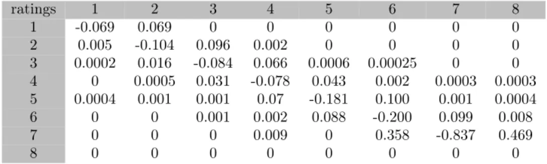
of the intensity approach where almost all transition probabilities were not null8. For instance, using a constant generator matrix on time interval[01/2013−01/2014]leads to the following results on the2013
one year transition matrix9, see Table4. 7See (35) in4.2to get the definition ofpˆ∗
ij.
8This difference is due to the fact that the cohort approach does not make full use of the available data. Specifically, the estimates of the cohort approach are not affected by the timing and sequencing of transitions within the period where the intensity approach captures within-period transitions.
1 2 3 4 5 6 7 8 1 87.13 12.77 0.10 0 0 0 0 0 2 0 98.57 1.39 0.04 0 0 0 0 3 0 1.57 93.59 4.78 0.06 0 0 0 4 0 0.03 3.17 94.29 2.36 0.15 0 0 5 0 0 0.13 7.56 89.50 2.71 0.08 0.02 6 0 0 0.01 0.68 9.31 83.68 4.84 1.48 7 0 0 0 0.05 0.82 14.13 59.60 25.40 8 0 0 0 0 0 0 0 100
Table 4: One year transition matrix on 2013
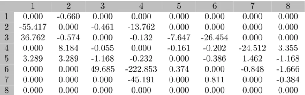
The transition matrix in Table4is typical of the migration dynamic behaviour. The probabilities on the diagonal are close to one which means that the ratings are quite stable during a short time period (which is the case for 1 year). The probabilities around the main diagonal (above and below) are also significant, while the other ones tend generally to zero. Indeed, during a short time period, a credit risk analyst has no incentive to downgrade (resp. upgrade) a rating for more than one grade. However, for the non investment grades, i.e. ratings 5, 6 and 7 it is common to have more heterogeneity than the investment grades. This is due in one hand to the financial situation of the firms standing at these ratings and in the other hand to the correction effect of agencies. When a default which has not been predicted by the rating agencies occurs, several adjustments are performed to correct for this prediction error, some downgrades are then applied to the firms which are in the same situation as the defaulted one. If we consider a constant matrix generator on the overall study period, i.e. [01/2006−01/2014] we get the following transition matrix that we can consider as a Through The Cycle transition matrix(see Table5). 1 2 3 4 5 6 7 8 1 92.69 6.47 0.48 0.03 0.31 0.02 0 0 2 0.64 89.93 8.96 0.46 0.01 0 0 0 3 0.02 1.47 92.37 5.91 0.20 0.03 0 0 4 0 0.08 3.12 92.13 4.16 0.41 0.06 0.04 5 0.06 0.09 0.25 6.89 83.99 8.16 0.41 0.15 6 0 0 0.13 0.52 7.96 82.77 6.10 2.52 7 0 0 0.03 0.61 1.24 22.92 43.27 31.93 8 0 0 0 0 0 0 0 100
Table 5: One year Through The Cycle transition matrix
Comparing to the2013 matrix, the TTC matrix is less concentrated on the diagonal and almost all the transition probabilities are not null. This is due to computation with respect to all the duration of data history, all the migrations are likely to happen during this time.
5.3
Estimation with observable factors
Many studies have addressed the question of selecting the appropriate covariates to explain time variation in the behaviour of ratings. This question is a large topic of investigation, one can refer to Kavvathas
(2001),Bangia et al.(2002),Couderc and Renault(2005) andKoopman et al.(2009) to have more details. In this study, we have followed the idea ofCouderc and Renault (2005) by selecting variables according to three covariates "families", i.e. macroeconomic information, financial and commodity markets infor-mation and credit market inforinfor-mation. As our portfolio is mainly composed of US and Euro positions we focused on US and Euro indicators. The entire list of covariates is given below10.
Macroeconomic variables : US and Euro Real Gross Domestic Product, US and Euro Consumer Price Indices, US and Euro Civilian Unemployment rates, US Effective Federal Funds rate (short term interest rate), Euro short term interest rates, US 10 years treasury constant maturity rate, long-term Government bond yields 10-years, US and Euro Industrial Production Indices, US and Euro Purchasing Manager Indices, Case-Shiller Index (real estate price Index for US).
10The macroeconomic indicators time series are in free access on the website of the FEDERAL RESERVE BANK OF ST. LOUIS, while the financial, commodity and credit indicators time series can be retrieved from Bloomberg.
Financial and commodity markets variables : Crude Oil price, Gold price, NASDAQ 100 Index, Dow Jones Index, Euro STOXX Index and Chicago Board Options Exchange Market Volatility Index.
Credit market variables : Bank of America Merrill Lynch US Corp BBB total return Index, Bank of America Merrill Lynch US Corp AA total return Index, Markit iBoxx AA and Markit iBoxx BBB.
The data time series go from01/2006to01/2014which encompasses our study period. Each variable consists in a year to year growth without overlapping between the sub-periods, this gives 8 sub-periods. For example, the US Real GDP growth for the date01/2014(last sub-period) is calculated as the relative variation during the period [31/12/2012−31/12/2013], which gives,
Real GDP Growth01/2014=
Real GDP31/12/2013− Real GDP31/12/2012
Real GDP31/12/2012
=15916 b$−15433b$
15433 b$ = 3.13%
As the number of covariates is important (25series), we have performed a Principal Component Analysis (PCA) in order to reduce the number of explicative factors. Table 6 summarizes the8 first eigenvalues with cumulated variance explained in percentage.
Eigenvalues Percentage of variance Cumulated percentage 8.79 43.99 43.99 3.39 16.98 60.98 2.43 12.19 73.18 1.61 8.09 81.27 0.95 4.77 86.04 0.72 3.64 89.69 0.56 2.83 92.53 0.36 1.83 94.36
Table 6: Observable factors eigenvalues
The first factor explains almost44%of the total variance, where the rest of factors (2until8) explain
50% cumulated variance. As there is not a strict rule to choose the number of covariates, we have inves-tigated the estimation procedure for different number of covariates. Above five factors the log-likelihood is no more significantly improved, we have then chosen thefive first factors with a cumulated explained variance of86%to realise the estimation procedure. The number of selected factors can be challenged in the light of a deeper investigation, but it is not the purpose of this paper.
5.3.1 Parameters estimation for the intensity model
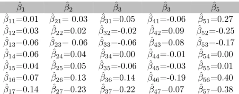
We recall that for the intensity model, the parameters to be estimated are the baseline intensity Λ0 (see
Table7) and the matrices of factor sensitivitiesβs,s= 1,· · · ,5 (see Table8below and Tables22-25in
appendixD.2). We use proposition3.4to estimate these parameters from the panel data composed of 8 sub-periods. 1 2 3 4 5 6 7 8 1 -0.03 0.03 0 0 0 0 0 0 2 0 -0.05 0.05 0 0 0 0 0 3 0 0.01 -0.07 0.06 0 0 0 0 4 0 0 0.03 -0.06 0.03 0 0 0 5 0 0 0 0.06 -0.13 0.07 0 0 6 0 0 0 0 0.10 -0.14 0.04 0 7 0 0 0 0 0 0.45 -0.72 0.27 8 0 0 0 0 0 0 0 0
1 2 3 4 5 6 7 8 1 0 -0.06 0 0 0 0 0 0 2 0.34 0 -0.11 1.58 0 0 0 0 3 -4.93 0.22 0 -0.03 0.28 2.77 0 0 4 0 12.38 0.02 0 -0.06 0.07 0.80 -2.47 5 -2.42 -2.42 -0.17 0.04 0 -0.04 -2.92 -0.17 6 0 0 -7.67 1.63 0.05 0 -0.04 -0.08 7 0 0 0 3.52 0 0.09 0 -0.11 8 0 0 0 0 0 0 0 0
Table 8: Beta for the first factor intensity model
In order to assess the statistical significance of theβˆij associated with the migrationi−→j, we have
implemented a likelihood ratio test11 consisting in the assessment of the null hypothesis H
0 : ˆβij,k =
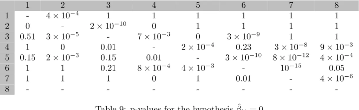
0, k = 1,· · ·,5 against the hypothesis H1 : ∃k ∈ {1,· · ·,5},βˆij,k 6= 0. Table 9 reports the p-values
associated with the likelihood ratio test.
1 2 3 4 5 6 7 8 1 - 4×10⁻⁴ 1 1 1 1 1 1 2 0 - 2×10⁻¹⁰ 0 1 1 1 1 3 0.51 3×10⁻⁵ - 7×10⁻³ 0 3×10⁻⁹ 1 1 4 1 0 0.01 - 2×10⁻⁴ 0.23 3×10⁻⁸ 9×10⁻³ 5 0.15 2×10⁻³ 0.15 0.01 - 3×10⁻¹⁰ 8×10⁻¹² 4×10⁻⁴ 6 1 1 0.21 8×10⁻⁴ 4×10⁻³ - 10−15 0.05 7 1 1 1 0 1 0.01 - 4×10⁻⁶ 8 - - -
-Table 9: p-values for the hypothesisβˆij = 0
The migrations are expected to be correlated with the business cycle, negatively when the migration is a downgrade and positively when the migration is an upgrade. According the Table 8, where the first factor can be considered as a proxy of the business cycle, this behaviour is confirmed for the short migrations (i.e. one grade migration, for instance βˆ12 = −0.06,βˆ23 = −0.11,βˆ32 = 0.22,βˆ21 = 0.34).
As can be seen on Table 9, the p-values associated with these sensitivities state for their statistical significance. When the migration is farther (i.e. more than two grades), due to the lack of observations, it is no more possible to state any significant relation with the business cycle (see the p-values associated to βˆ31,βˆ51,βˆ46, βˆ63). When we focus on the non investment grade obligors (ratings 5, 6 and 7), we can
observe that, all downgrades are significantly negatively correlated to the business cycle, whatever the amplitude of the migration (see the p-value associated withβˆ57,βˆ58,βˆ68, etc).
5.3.2 Parameters estimation for the structural model
For the structural model, the parameters are θ = (Ci+1, αi, βi, σi)i=1,···,7, these parameters where
esti-mated using the equations (9 -11). The results are reported in Tables10and11.
ˆ C αˆ σˆ ˆ C2= 5.16 αˆ1= 5.08 σˆ1= 0.17 ˆ C3= 4.35 αˆ2=3.83 σˆ2= 0.38 ˆ C4= 3.47 αˆ3= 3.14 σˆ3= 0.74 ˆ C5= 2.16 αˆ4= 2.47 σˆ4= 1.18 ˆ C6= 1.05 αˆ5= 1.52 σˆ5= 1.17 ˆ C7 = -0.19 αˆ6=0.63 σˆ6= 1.17 ˆ C8 = -1.55 αˆ7=-1.01 σˆ7= 1.72
Table 10: Parameters for observable factors structural model 11SeeLando and Skodeberg(2002) for more details about the test.
ˆ β1 βˆ2 βˆ3 βˆ3 βˆ5 ˆ β11=0.01 βˆ21= 0.03 βˆ31=0.05 βˆ41=-0.06 βˆ51=0.27 ˆ β12=0.03 βˆ22=0.02 βˆ32=-0.02 βˆ42=0.09 βˆ52=-0.25 ˆ β13=0.06 βˆ23= 0.06 βˆ33=-0.06 βˆ43=0.08 βˆ53=-0.17 ˆ β14=0.06 βˆ24=0.04 βˆ34=0.00 βˆ44=-0.01 βˆ54=0.00 ˆ β15=0.04 βˆ25=0.05 βˆ35=-0.06 βˆ45=-0.03 βˆ55=0.01 ˆ β16=0.07 βˆ26=0.13 βˆ36=0.14 βˆ46=-0.19 βˆ56=0.40 ˆ β17=0.14 βˆ27=0.23 βˆ37=0.22 βˆ47=0.07 βˆ57=0.38
Table 11: Beta for observable factors structural model
The likelihood ratio test has also been implemented for the structural model. For any i = 1· · · ,7
and k= 1,· · ·,5, we consider the null hypothesis given by H0 : ˆβik= 0. The p-values of these tests are
reported in Table12. ˆ β1 βˆ2 βˆ3 βˆ3 βˆ5 1 0.10 0.02 0.05 9×10⁻⁵ 10−5 1 0.30 10−5 1 5×10⁻⁸ 10−4 6×10⁻⁴ 10−3 1 2×10⁻³ 9×10⁻³ 1 0.60 1 2×10⁻³ 0.01 4×10⁻³ 0.30 0.50 10−4 5×10⁻¹¹ 4×10⁻⁷ 8×10⁻⁸ 6×10⁻¹⁰ 0.01 2×10⁻¹⁰ 0.04 0.03 5×10⁻³
Table 12: p-values for hypothesisβˆik= 0
The results of Tables10,11and12are consistent with those obtained byGagliardini and Gourieroux
(2005) as the estimated barrier levels Cˆ increase with respect to rating quality. The same conclusion holds for the intercepts αˆi which confirms that the downgrade risk is higher for low quality credit. The
estimated rating volatilities are consistent with the fact that the non investment grade firms are likely to move in a larger set of ratings. Indeed, σˆ7= 1.72andσˆ6= 1.17, whereasσˆ1= 0.17andσˆ2= 0.38. One
should also notice that the βˆ coefficients for the non investment grade ratings6 and 7 are significantly higher than for the investment grade firms. As can be seen in Table 12, they are also statistically more significant. These results confirm that the weakest firms are more impacted by adverse changes in the economy.
5.4
Estimation with unobservable latent factors
The use of latent factors to explain time variation of the credit ratings requires to compute a relatively high number of empirical transition intensities λˆij,t, i ∈ {1,· · ·,7}, j ∈ {1,· · ·,8}, i6=j. Indeed, λˆij,t
are used as inputs for both models, they are transformed into ψˆiJ,t for the structural model (see next
section) and kept as such for the intensity model. In order to increase the number of observations, we have considered an overlapping year to year sub-period with one month slope. With8 years of monthly frequency data, this allows to have86observations instead of8 observations if the sub-periods were not overlapping12. For instance,λˆij,t
1 is calculated on the sub-period[01/2006−01/2007],λˆij,t2 is calculated
on the sub-period [02/2006−02/2007], etc. We recall thatˆλij,t are computed using the proposition3.3.
5.4.1 Determining the number of unobservable factors
Since the covariates are unobserved we proceed by using the method proposed inGagliardini and Gourier-oux(2005) to find the number of covariates in both structural and intensity models. The idea is to build time series ofλˆij,t andψˆiJ,t fort=t1,· · ·, t86, to consider them as the realisations of random variables
and then carry on a PCA to find the number of common factors.
For the intensity model, we count49variablesλˆ12,t,λˆ13,t,· · · ,λˆ78,t, each one going fromt1tot86which
makes49time series. The PCA is then applied on this set to compute the common factors. Concerning the structural model, theλˆij,tare transformed into empirical transition probabilitiespˆij,t using (5), then
12We need a high number of observations in order to perform the Kalman filter, we have performed the Kalman filter on 8 observations but we didn’t get a satisfying result.
the series ψˆiJ,t such as ψˆiJ,t = Φ−1 pˆ∗iJ,t
for t =t1,· · ·, t86 are computed (see (35) in 4.2 to get the
definition of pˆ∗iJ,t ). We get also49times series on which we apply the PCA. The corresponding eigenvalues are given in decreasing order in the Table13.
intensity eigenvalues Cumulated percentage structural eigenvalues Cumulated percentage 1.83 79.50 1853.46 48.89 0.43 98.28 735.23 72.29 0.02 99.27 515.81 81.52 0.007 99.58 311.41 89.04 0.003 99.71 306.01 93.81 0.002 99.82 247.94 96.50 Table 13: Eigenvalues
For the λˆij,t time series, the first two factors explain 98% of the total variance. The variance of ψˆiJ,t
time series are explained at 72%by the two first factors. In order to choose the number of processes to use in the Kalman filter we have estimated two models, the first with one common factor and the second with two common factors. We found that in both cases, the first filtered process was the same, the second filtered process of the model with two common factors was identical to the first one with respect to a scale factor. According to these elements we have chosen the model with one common factor. The filtered process obtained was considered as the business cycle. Once the number of covariates known, we have done the parameters estimation using the two steps procedure, filtering of the process X¯t and
maximisation of the log-likelihood (see subsections 3.3and 4.2). We present and discuss the results for the one factor models below.
5.4.2 Results and discussion
We report in the Figures 1 and 2 the filtered processes E(Xt | Yt) and E(Xt | Ψt) respectively13, for
t=t1,· · · , t86. Recall thatE(Xt|Yt)andE(Xt|Ψt)correspond to the filtered factor process associated
with max-likelihood models (see (3.4) and (4.2)). The figures below clearly show periods ofpeak,normal
times and trough which are properties of the business cycle. Our period of study encompasses what it is known as the Liquidity Crisis and Sovereign Debt Crisis, with some famous events like the Lehman Brothers bankruptcy on September2008and the falls of market indices like CAC40, DAX and FTSE100
during the summer 2011. As can be seen on Figures 1 and2, the Liquidity Crisis seems to be captured by both models. Note that, during theSovereign Debt Crisis, the decrease of the filtered factor process is higher in the structural model than in the intensity model.
13Note that the process
Figure 1: Filtered common factor in the intensity model
Figure 2: Filtered common factor in the structural model
5.4.3 Parameters estimation for the intensity model
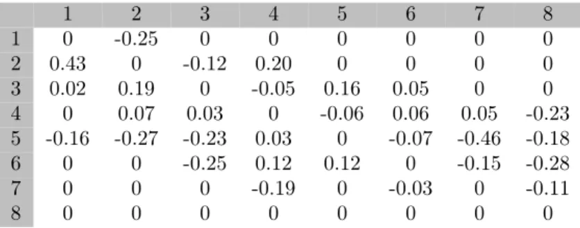
The estimated parameters and the p-values for the one factor intensity model are reported in Tables 14,
15and16. 1 2 3 4 5 6 7 8 1 -0.03 0.03 0 0 0 0 0 0 2 0 -0.08 0.08 0 0 0 0 0 3 0 0 -0.07 0.07 0 0 0 0 4 0 0 0.03 -0.07 0.04 0 0 0 5 0 0 0 0.07 -0.17 0.1 0 0 6 0 0 0 0 0.07 -0.15 0.08 0 7 0 0 0 0 0 0.27 -0.67 0.42 8 0 0 0 0 0 0 0 0
Table 14: Baseline intensity for one factor intensity model 1 2 3 4 5 6 7 8 1 0 -0.25 0 0 0 0 0 0 2 0.43 0 -0.12 0.20 0 0 0 0 3 0.02 0.19 0 -0.05 0.16 0.05 0 0 4 0 0.07 0.03 0 -0.06 0.06 0.05 -0.23 5 -0.16 -0.27 -0.23 0.03 0 -0.07 -0.46 -0.18 6 0 0 -0.25 0.12 0.12 0 -0.15 -0.28 7 0 0 0 -0.19 0 -0.03 0 -0.11 8 0 0 0 0 0 0 0 0
Table 15: Beta for one factor intensity model
1 2 3 4 5 6 7 8 1 - 3×10⁻³ 1 1 1 1 1 1 2 4×10⁻⁴ - 6×10⁻⁹ 0.12 1 1 1 1 3 1 5×10⁻⁶ - 6×10⁻³ 0.05 0.72 1 1 4 1 1 0.20 - 4×10⁻³ 0.33 0.54 0.09 5 0.87 0.21 0.14 0.10 - 2×10⁻⁴ 10−4 0.06 6 1 1 0.22 0.27 3×10⁻³ - 10−16 10−3 7 1 1 1 0.2 1 0.01 - 6×10⁻⁶ 8 - - -
-Table 16: p-values for hypothesisβˆij = 0
5.4.4 Parameters estimation for the structural model
The estimated parameters and the p-values for the one factor structural model are reported in Tables17
and18. ˆ C αˆ σˆ βˆ ˆ C2 = 6.82 αˆ1= 5.01 σˆ1= 1.71 βˆ1= 0.43 ˆ C3 = 4.50 αˆ2= 3.12 σˆ2= 0.76 βˆ2= 0.10 ˆ C4 = 3.12 αˆ3= 2.56 σˆ3= 0.69 βˆ3= -0.06 ˆ C5 = 1.84 αˆ4= 1.83 σˆ4= 0.69 βˆ4= -0.05 ˆ C6 = 0.96 αˆ5= 1.23 σˆ5= 0.75 βˆ5= 0.03 ˆ C7= 0.001 αˆ6= 0.12 σˆ6= 0.87 βˆ6= 0.03 ˆ C8 = -0.43 αˆ7= -0.56 σˆ7= 1.09 βˆ7= -0.03
Table 17: Parameters for one factor structural model
For anyi= 1,· · · ,7, we test the null hypothesisH0: ˆβi= 0. The corresponding p-values are reported
in Table18.
ˆ
β1= 0 βˆ2= 0 βˆ3= 0 βˆ4= 0 βˆ5= 0 βˆ6= 0 βˆ7= 0
1 0 0 6.6×10⁻¹⁶ 1 1.1×10⁻¹⁶ 0.01 Table 18: p-values for hypothesisβi= 0
The parameters obtained for both models are consistent with those obtained in the case of observable factors. However, note that, for the structural model, the null hypothesis cannot be rejected for the beta’s associated with the first and the fifth rating class.
5.5
Comparison between models
As stated previously, the aim of this paper is to assess and compare the migration models on their ability to link the transition probabilities to dynamic risk factors. In order to achieve this objective, we proceed in two steps. First, we compare the one year default probabilities implied by each model during the study period with the empirical default probabilities. We have chosen the default probability
because this indicator is the most relevant from the credit risk perspective. Nevertheless, other transition probabilities have been compared and reported into appendixD.5(see Figures 9, 10,11,12,13). These results are in the same line as the one obtained for default probabilities. Secondly, we compare transition matrices of each model with respect to a metric called SVD mobility index and introduced inJafry and Schuermann(2004). The mobility index is a function that measures the ability of a transition matrix to generate migration events (the mobility index is detailed in subsection5.5.2). The model parameters used for the computation of one-year default probabilities and mobility indices are those obtained from the estimation procedures of the two previous sections (observable and latent covariates). The comparison is made with respect to a credit migration model with no covariate – called theempirical model hereafter – where, on each sub-period, the transition matrix is estimated using the procedure described in proposition
3.3(see also subsection5.2). Recall that we have 8 non overlapping sub-periods for the observable factors and 86 overlapping sub-periods for the unobservable factors.
5.5.1 Comparison using the implied one year default probabilities
We compute the one year matrices implied on each sub-period by both intensity and structural models. We present graphically the evolution of the implied default probabilities of the ratings 4, 5, 6 and 7 (the default probabilities of the ratings 1, 2, and 3 are almost null).
Observable factors: Figures 3 and 4 represent the estimated one year default probabilities in the empirical model (solid line), in the intensity model (dashed line) and in the structural model (dotted line). One can see on the Figure 3 that for ratings 4 and 5 the intensity model adjusts perfectly the empirical default probabilities, the curves are almost identical. The structural model over-estimates the default probabilities for the rating 5, when the curve of the default probabilities for the rating 4 is almost flat.
Figure 3: Ratings 4 and 5: implied one year default probabilities. Model estimation performed in the case of observable factors. Empirical model in solid line, intensity model in dashed line, structural model in dotted line.
On the Figure4 the same observation is made with regards to ratings 6 and 7. The intensity model fits very well the empirical default probabilities when the structural model over-estimates them.
Figure 4: Ratings 6 and 7: implied one year default probabilities. Model estimation performed in the case of observable factors. Empirical model in solid line, intensity model in dashed line, structural model in dotted line.
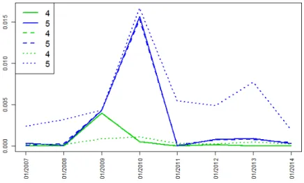
Unobservable factors: Figure 5 shows that both models are not able to reproduce the one year empirical PD during the trough period, see the period[01/2009−07/2010]. Concerning the rest of the study period, the structural model over-estimates the PD for the rating 5 where it shows an almost flat curve for the PD rating 4. The PD curves of the intensity model (for ratings 4 and 5) are most of the time under the empirical PD.
Figure 5: Ratings 4 and 5: implied one year default probabilities. Model estimation performed in the case of unobservable factors. Empirical model in solid line, intensity model in dashed line, structural model in dotted line.
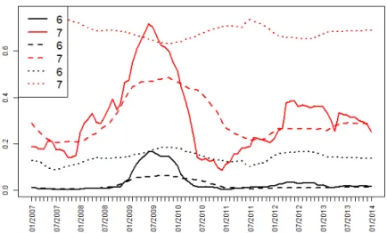
Concerning the one year PD for the ratings 6 and 7 (see Figure 6), the structural model shows a quasi non sensitivity to the business cycle. Indeed, the curves are high and almost flat comparing to the empirical one year PD. The intensity model shows a better adjustment in the sense that it is more reactive than the structural model to the business cycle but it is still unable to reproduce the empirical PD during thetrough period.
Figure 6: Ratings 6 and 7: implied one year default probabilities. Model estimation performed in the case of unobservable factors. Empirical model in solid line, intensity model in dashed line, structural model in dotted line.
5.5.2 Comparison using the SVD mobility index
In literature, comparing transition matrices is usually done using three methods, the euclidean distance (seeIsrael et al.(2001)), statistic testing, t-test orχ2(seeNickell et al.(2000),Foulcher et al.(2004)) or with a mobility index (seeGeweke et al.(1986),Jafry and Schuermann(2004)). The mobility index was introduced to compare two transition matrices on their ability to generate migration events. It is defined as a function M(Π)ofRd×d−→Rwhere by convention M(I) = 0, withI the identity matrix. A good
mobility index must be assessed on three criteria, persistence, convergence and temporal aggregation (see the well documented papers of Shorrocks (1978), Geweke et al. (1986) andJafry and Schuermann
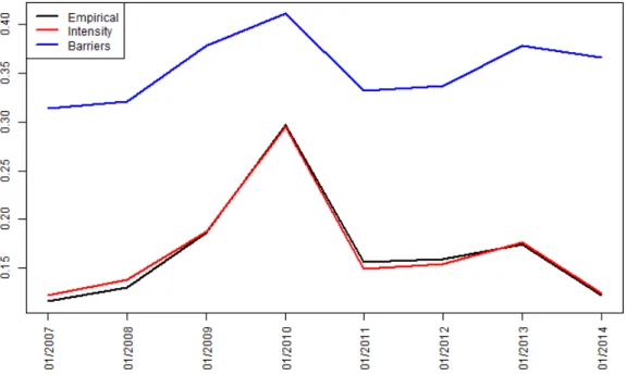
(2004) to have a complete overview of this topic). In this paper we use the mobility index instead of the euclidean distance or the statistic testing because the latter are relative measures : the comparison is then only possible between two matrices. In contrast, the mobility index is an absolute measure, all transition matrices can be compared according to it. Morever, the mobility index has an intuitive interpretation, the higher it is, the more dynamic the transition matrix is. We present hereafter the SVD mobility index introduced inJafry and Schuermann (2004). This metric will be used to compare the matrices implied by the intensity and the structural models when factors are observable and when factors are unobservable.
For ad-dimensional square matrixΠ, the SVD mobility index is given by,
MSV D(Π) = Pd i=1 r λi ˜ Π0Π˜ d , (40)
where Π = Π˜ −I and Π˜0 is its transpose. λi
˜
Π0Π˜is the ith eigenvalue of Π˜0Π˜, sorted in decreasing
order, i.e. λ1( ˜Π0Π)˜ >· · ·> λd( ˜Π0Π)˜ .
We have applied the SVD mobility index on each matrix calculated according to the intensity and structural models. Figures 7 and 8 show the evolution of the SVD mobility index of the empirical model (black curve), of the on intensity model (red curve) and of the structural model (blue curve). Figure7corresponds to estimations with observable factors whereas Figure8corresponds to estimations with unobservable factors. The two figures confirm the statements made previously : the intensity model with observable factors fits very well the empirical transition matrices whereas the other models, i.e., the structural with observable factors, the intensity with latent covariates and the structural with latent covariates, over-estimates, under-estimates and over-estimates respectively the empirical transition matrices.
Figure 7: Implied SVD mobility index implied when model estimation is performed in the case of observ-able factors. Empirical model in black, intensity model in red, structural model in blue.
Figure 8: Implied SVD mobility index implied when model estimation is performed in the case of unob-servable factors. Empirical model in black, intensity model in red, structural model in blue.
As a conclusion for the subsection5.5we can state that the intensity model with observable factors is the one that best fits the empirical probabilities. This is mainly due to following points:
• for the intensity model with observable factors, the parametersλij,0andβij are estimated through
factors, it is most likely to have at least one factor that explains correctly the intensity migration
λij. The estimation of the structural model parameters is done through the maximization of the
global likelihood function, this is less tractable than the intensity model in the sens that it is not possible to explain separately the transition probabilities.
• for the intensity model with observable factors, the maximum likelihood problem is solved using a semi-analytical solution which is not the case of the other models. Indeed the baseline intensity estimatorˆλij,0is given analytically when the regression coefficientsβˆare obtained through the
res-olution of the gradient of the log-likelihood function which represents a simple non-linear equations system. The parameters of the structural model with observable factors are also estimated through the resolution of the gradient of the log-likelihood function but the non-linear equations system is far more difficult to resolve.
• for the statistical estimation using unobservable factors, the solution ofGagliardini and Gourieroux
(2005) to skip the issue of high dimension integrals requires to build a linear Gaussian model to apply the Kalman filter. The assumption of an infinite number of obligors n and the asymptotic normality of the maximum likelihood estimator at each time t and for every migration (i,j) is not satisfied. Indeed, even with a very high value of n, some migrations are unlikely to happen frequently like the long migrations (three grades or more). The intensity model with observable factors uses directly the observations without making some approximations based on very restrictive assumptions.
• the latent factors models have more parameters to estimate (the filtered processX¯tand the
auto-regression matrixA). This constraint added to the limited quantity of data plays an important role in the final results.
6
Conclusion
The aim of this paper is to assess and compare two alternative stochastic migration models on their ability to link the transition probabilities to either observable or unobservable dynamic risk factors. In this respect, we use the same data set (S&P credit ratings on the period [01/2006−01/2014]) to estimate model parameters in the multi-state latent factor intensity model and in the ordered Probit model. The estimation procedure is detailed in the two cases where the underlying dynamic factors are assumed to be either observable or unobervable. When the underlying factors are unobservable, we adapt a method given inGagliardini and Gourieroux(2005) to represent the considered factor migration model as a linear Gaussian model. In that case, we identify the business cycle as the factor process filtered by a standard Kalman filter. The estimation methods are compared on their ability to fit the one-year empirical default probabilities and their ability to reproduce the empirical SVD mobility index. We conclude that the intensity model with observable factors was the one which best fits the S&P rating history. In line withKavvathas(2001), this study shows that short migrations of investment grade firms are significantly correlated to the business cycle whereas, because of lack of observations, it is not possible to state any relation between long migrations (more than two grades) and the business cycle. Concerning non investment grade firms, downgrade migrations are negatively related to business cycle whatever the amplitude of the migration.
References
Albanese, C., Campolieti, G., Chen, O., and Zavidonov, A. (2003). Credit barrier models.Risk Magazine, 16:109–113.
Bangia, A., Diebold, F., and Schuermann, T. (2002). Ratings migration and the business cycle, with application to credit portfolio stress testing. Journal of Banking and Finance, 26:445–474.
Couderc, F. and Renault, O. (2005). Business and financial indicators: W