Extending the SACOC algorithm through the
Nystr¨
om method for Dense Manifold Data
Analysis
H´
ector D. Men´
endez
Department of Computer Science, University College London, United Kingdom Tel.: +44 (0)2031 084042 E-mail: [email protected]
Fernando E. B. Otero
School of Computing, University of Kent, United Kingdom Tel.: +44 (0)1634 888822 E-mail: [email protected]
David Camacho
Department of Computer Science, Universidad Aut´onoma de Madrid, Spain Tel.: +34 91 497 22 88 E-mail:[email protected]
Abstract: Data analysis has become an important field over the last decades. The growing amount of data demands new analytical methodologies in order to extract relevant knowledge. Clustering is one of the most competitive techniques in this context. Using a dataset as a starting point, these techniques aim to blindly group the data by similarity. Among the di↵erent areas, manifold identification is currently gaining importance. Spectral-based methods, which are the mostly used methodologies in this area, are however sensitive to metric parameters and noise. In order to solve these problems, new bio-inspired techniques have been combined with di↵erent heuristics to perform the clustering solutions and stability, specially for dense datasets. Ant Colony Optimization (ACO) is one of these new bio-inspired methodologies. This paper presents an extension of a previous algorithm named Spectral-based ACO Clustering (SACOC). SACOC is a spectral-based clustering methodology used for manifold identification. This work is focused on improving this algorithm through the Nystr¨om extension. The new algorithm, named SACON, is able to deal with Dense Data problems. We have evaluated the performance of this new approach comparing it with online clustering algorithms and the Nystr¨om extension of the Spectral Clustering algorithm using several datasets. Keywords: Ant Colony Optimization, Clustering, Data Mining, Machine Learning, Spectral, Nystr¨om, SACON, SACOC
1 Introduction
Data analysis is currently a growing field [1]. The importance of analysing these data quantities is growing as a consequence of Social interactions, smart devices, WiFi and networks, etc. Several methodologies have been extended in order to deal with these problems. Two of the most recent methodologies in Data Mining are based on MapReduce [1] and online algorithms [2]. The former is an approach which was designed for parallelizing computation. Using several nodes it distributes some calculus in two steps the mapper and the reducer step. Online analysis is a methodology where data instances are only processed once and the system keeps no information about old instances. This reduces the memory usage and allows the algorithms to work with Dense Data.
There are several Data Mining approaches which deal with Dense Data. The most relevant are those based on
Supervised [3] and Unsupervised Learning [3]. Because supervised techniques usually need human assistant by a manual labelling process, and this is costly, unsupervised techniques are gaining importance in this area [2]. One of the most relevant unsupervised techniques is clustering. Clustering is defined as the process of grouping data blindly, using a similarity criterion. These methods have been extensively used in several and heterogeneous fields [3].
Clustering techniques can be divided in several sub-areas [3] such as centroid-based, medoid-based, hierarchical and continuity-based among others. This work is based on the latter. Continuity-based clustering is a methodology focused on the identification of manifolds within the data. These manifolds are structures which are defined by the data points inside their search space [4]. The main idea behind this work is to extend a previous continuity-based algorithm to a
Copyright c 2008 Inderscience Enterprises Ltd. Copyright c 2009 Inderscience Enterprises Ltd.
Dense Data approach. The algorithm, named SACOC (Spectral-based ACO Clustering algorithm) [5], is a bio-inspired clustering algorithm based on Ant Colony Optimization.
Ant Colony Optimization [6] algorithms are based on the foraging behaviour of the ants when they need to find the shortest path between their nest and the food source. The ants use a methodology based on pheromones to indicate the path that they have followed. The evaporation of these pheromones is used to choose the best path. This idea can be extended to optimization problems and has been successfully applied in several fields, such as Data Mining [7, 8].
This work aims to extend a previous SACOC the Nystr¨om extension [9]. This extension applies a space reduction using a subset of the dataset. It guarantees accurate solutions even when the reduction has been applied. The new algorithm designed, called SACON, has been evaluated using several continuity-based datasets and it has been compared against Online Clustering algorithms and the Nystr¨om extension of Spectral Clustering.
The paper is structured as follows: Section 2 presents the related work, Section 3 introduces the SACOC algorithm which is extended in Section 4 to create the new SACON algorithm. Section 5 shows the experimental setup applied in the experiments of Section 6. Finally, the last section explains the conclusions.
2 Related Work
Following sections will be focused on provide a general description of the clustering problem, include some issues about ACO for classification and clustering.
2.1 Clustering Large Data
Clustering has been widely used in several and heterogeneous fields. Important challenges of large data analysis is the online analysis. Clustering methods have become promising techniques in this field, as these algorithms can deal with unlabelled data.
The idea behind online clustering algorithm is to analyse this data using real-time techniques. These techniques usually need to deal with large data quantities. The main problem of these algorithms is that they need a specific space to update the information. This limits the possibilities of the new algorithm, producing for example, that some clustering algorithms might not be easily adapted to this kind of analysis [2].
One of the main tools used for online clustering analysis is the Massive On-line Analysis (MOA) tool. This framework provides the following online clustering algorithms:
• Online K-means [2]: This online algorithm updates the centroid position when a new instance arrives. Only one centroid is updated per iteration. It is similar to classical K-means algorithm.
• ClusTree [10]: This online algorithm iteratively updates the information of the clusters. It is able to consider the speed of the data stream generating the concept of the age of the object. It also maintains stream summaries.
• CluStream [11]: This algorithm combines o✏ine clustering and online clustering in order to provide partial clustering solutions which measure the evolution of the clusters.
All of these algorithms have been designed in order to identify more properties of the data stream than the final clusters in a specific moment.
2.2 Continuity-based and Spectral Clustering
This section explains the Spectral Clustering Algorithm (see Algorithm 1) which is one of the most relevant continuity-based clustering algorithms. The algorithm starts generating a Similarity Graph among the data instances (line 1 of Algorithm 1), pair to pair. There are three main methodologies, i.e., graphs, which are used in these techniques [12]:1. The ✏-neighbourhood graph: all the components whose pairwise distance is smaller than✏ are connected.
2. The k-nearest neighbour graphs: the vertex vi is connected with vertex vj if vj is among the k-nearest neighbours ofvi.
3. The fully connected graph: all points with positive similarity are connected with each other. This work is centred in the fully connected graph. One of the most important metrics used in Spectral Clustering is the RBF kernel [14] defined by:
s(xi, xj) =e ||xi xj||
2
(1) The second step is related to the study of the eigenvectors of the Laplacian Matrix of the Similarity Graph (lines 2 and 3 of Algorithm 1). Depending on the Laplacian Matrix calculation, there are three di↵erent techniques related to Spectral Clustering [12]:
1. Unnormalized Spectral Clustering It defines the Laplacian matrix as:L=D W
2. Normalized Spectral ClusteringIt defines the Laplacian matrix as:Lsym=D 1/2LD 1/2=I D 1/2W D 1/2
3. Random Walks-based Normalized Spectral Clustering It defines the Laplacian matrix as: Lrw=D 1L=I D 1W
In these equationsIis the identity matrix,Drepresents the diagonal matrix whose (i, i)-element is the sum of the Similarity Matrix ith row and W represents the Similarity Graph (see Algorithm 1, line 2). Once the
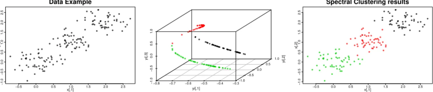
−0.5 0.0 0.5 1.0 1.5 2.0 2.5 − 1.0 − 0.5 0.0 0.5 1.0 1.5 2.0 2.5 Data Example x[,1] x[,2] −0.8 −0.7 −0.6 −0.5 −0.4 −0.3 − 1.0 − 0.5 0.0 0.5 1.0 −1.0 −0.5 0.0 0.5 1.0 yi[,1] yi[,2] yi[,3] −0.5 0.0 0.5 1.0 1.5 2.0 2.5 − 1.0 − 0.5 0.0 0.5 1.0 1.5 2.0 2.5
Spectral Clustering results
x[,1]
x[,2]
Figure 1 Spectral Clustering process from the original dataset to the final clustering results (left to right): the original data, the partition in the projective space and the final discrimination.
Algorithm 1Normalized Spectral Clustering according to Ng et al. (2001)[13]
Require: A dataset of n elements X ={x1, . . . , xn} and a fixed number of clustersk.
Ensure: A set of clusters C={C1, . . . , Ck} which is a partition ofX
1: Form the Similarity Graph W 2Rn⇥n defined by Wij =e ||xi xj||
2
ifi6=j, andWii = 0.
2: Define D to be the diagonal matrix whose (i, i)-element is the sum of thei-th row ofW.
3: Construct the matrixL=D 1/2W D 1/2.
4: Find v1, . . . , vk, the k largest eigenvectors of L (chosen to be orthogonal to each other in the case of repeated eigenvalues) and form the matrix V = [v1v2. . . vk]2Rn⇥k by stacking the eigenvectors in columns.
5: Form the matrix Y from V by renormalizing
each row of V to have unit length (i.e. Yij = Vij/(PjVij2)1/2).
6: Apply K-means (or any other algorithm) treating each row ofY as a point in Rk.
7: Assign the points xi to clusterCj if and only if the rowiof the matrixY was assigned to cluster j.
8: return C
Laplacian is calculated (in Algorithm 1 the Normalized Spectral Clustering algorithm is used), its eigenvectors are extracted (see lines 4 and 5 of Algorithm 1). Some of the main problems of Spectral Clustering are related to the consistency of the two classical methods used in the analysis: normalized and un-normalized Spectral Clustering. A deep analysis about the theoretical e↵ectiveness of normalized clustering over un-normalized can be found in [15].
The graph cut problem is closely related to Spectral Clustering. In the graph cut literature this problem has two classical solutions [12]: RadioCut and NCut. Von Luxburg et al. [12] describe the connection between the di↵erent approaches of Spectral Clustering (focused on the Laplacian Matrices), RadioCut and NCut. They also show that Unnormalized Spectral Clustering converges to RadioCut and the Normalized methods converge to NCut.
Figure 1 shows an example where the Laplacian Matrix has a maximum of 150 di↵erent eigenvectors.
According to the leader eigenvalues (those eigenvalues with the highest values) their associated eigenvectors are chosen. Since this example has three clusters (see Figure 1), the 3 leader eigenvectors are chosen.
The last step is the application of a clustering algorithm to the projective space formed by the normalized eigenvectors (see Figure 1 considering each row of the matrix as a point (see lines 6 and 7 of Algorithm 1). The most frequently applied algorithm is K-means. There are several versions of Spectral Clustering according to the algorithm that is used in this step, e.g., the SACOC [5] algorithm is a Spectral-based algorithm which applies an ACO clustering algorithm instead of K-means. Figure 1 shows the application of K-means to the previous example. The figure shows the distribution of the data in the space generated by the chosen eigenvector. In this case, each point could be interpreted as a projection of the original points. The results of the application of the algorithm to this data are also shown in Figure ?? (right). The data in the projective space is easier to separate than in the original space. This shows the results of the algorithm in the original space.
The main problem of Spectral Clustering is how to compute the eigenvectors and the eigenvalues of the Laplacian Matrix of the Similarity Graph avoiding the huge memory that it consumes. For example, when large datasets are analysed, the Similarity Graph of the SC algorithm requires a high memory storage and it makes extremely hard the eigenvalues and eigenvectors computation.
2.3 Ant Colony Optimization in Classification
and Clustering
One of the current perspectives which deals with Machine Learning problems is Ant Colony Optimization [6]. ACO approaches have been used to improve local minima convergence problems. These algorithms are designed to look for an optimal solution. These approaches have been applied for both, classification [3] and clustering [3] algorithms.
In ACO there are also some adaptations of classification algorithms—e.g., Otero et al. introduce an ACO algorithm for decision tree induction [7]; Blum and Socha introduce a neural network ACO model [16] and
Centroid 1 Centroid 2 Centroid 3
Int. 1 Int. 2 Int. 3 Int. 4 Int. 5 Figure 2 The construction graph of SACOC. The arrows
represent a trail of an ant.
Borrotti and Poli focused their work on the Na¨ıve Bayes model [17].
There are also some clustering algorithms which have produced promising results—e.g., Kao and Cheng designed a centroid-based ACO clustering algorithm [18]; Ashok and Messinger focused their work on graph-based clustering [19]; Men´endez et al. designed a Medoid-based ACO Clustering algorithm called MACOC [8] focused on improving the results of ACOC; and, finally, several other approaches are discussed in [20]. It is interesting to remark that both MACOC and SACOC are based on ACOC algorithm. The logic of the algorithms is similar (also the parameters), but the goal and search space are di↵erent.
3 Spectral-based
ACO
Clustering
Algorithm (SACOC)
This section presents the Spectral-based ACO Clustering Algorithm (SACOC) [5]. This algorithm is similar to Spectral Clustering. The goal of the algorithm is to choose the data discrimination representing the information as a Similarity Graph, and cutting it in di↵erent clusters.
3.1 ACOC algorithm
The ACOC algorithm (see Algorithm 2) is the base of SACOC (see Algorithm 3). It has a search space based on instances and centroids, and can be defined as a graph whose associated matrix is a N⇥k matrix, where N is the number of instances and k is the number of centroids (clusters).
The algorithm works with several ants looking for the best path in the graph (see Fig. 2). Each ant (a) has the following features: a list of visited objects (tba), a set of chosen centroidsCa and a Weighted matrixWa (related to the assignment of objects to clusters).
An ant a has two possible strategies: exploration and exploitation. It chooses the strategy according to the following equation:
j= ⇢
argmaxu2Ni{[⌧(i, u)][⌘a(i, u)] }, if qq0
S , otherwise ,(2)
whereNiis the set of nodes associated to objecti,jis the chosen cluster,⌧(i, u) is the pheromone value betweeni
and u,q0 is the exploitation probability,q is a random number for strategy selection, is a parameter, ⌘k(i, u) is the heuristic value between iand ufor antadefined by the formula: ⌘a(i, u) = 1/d(x
i, caj).
wherexi is a data instance andckj is a centroid from the ant centroid list. andS is the exploration defined by:
S=Pa(i, u) =P[⌧(i, u)][⌘a(i, u)] m
j=1[⌧(i, j)][⌘a(i, j)]
. (3)
The algorithm steps can be divided by:
1. Initialize pheromone matrix (see line 1 of Algorithm 2).
2. Initialize ants (see line 3 of Algorithm 2): (tba,Ca, Wa), for each ant ain the colony. Then, each ant repeats untiltba is full:
(a) Select (randomly) a data object i satisfying i /2tba (see line 6 of Algorithm 2).
(b) Select a cluster j: first the ant chooses a strategy; then, it calculates the transition probability and, finally, it visits a node (see line 7 of Algorithm 2).
(c) Updatetba,Ca andWa(see lines 9 and 10 of Algorithm 2).
3. Choose the best solution. First, calculate the objective function for each ant (see lines 14 and 15 of Algorithm 2): Jk= n X i=1 m X j=1 waijd(xi, caj) , (4) where wa
ij is a weight value of the assignment matrixWa. Next, rank ants solutions. Choose the iteration-best solution, apply local search (for more details of local search see [21]), to improve the solution and, finally, compare it with the best-so-far solution and update this value with their maximum.
4. Update pheromone trails (global updating rule). Only the bestr ants are able to add pheromones. Let ⇢ be the pheromone evaporation rate, (0<
⇢<1), t the iteration number, r is the number of elitism ants and ⌧h
ij = 1/Jh (see line 17 of Algorithm 2): ⌧ij(t+ 1) = (1 ⇢)⌧ij(t) + r X h=1 whij ⌧ijh . (5)
5. Check the termination condition: if the number of iterations is greater than the maximum limit, finish; otherwise, go to step 2.
Algorithm 2ACOC algorithm.
Require: X =x1, . . . , xn andknumber of clusters Ensure: c1, . . . , ck bestk centroids
1: Initialize the pheromone matrix⌧0.
2: forgenerationg= 0tomaxGenerationsdo
3: Initialize ants:Ca=
;andtba =
; 4: for allanta2A(the ants set)do
5: while|tba|==nor|Ca|==kdo
6: Select the next data objecti
7: Choose a strategy (exploration,
exploitation)
8: Selectcq⇤ 2Ca as the closest centroid
9: SetWi,qa⇤ = 1
10: addInstance(i) totba 11: end while
12: Calculate the objective function for each
ant:Ja=Pn i=1min|
M|
j=1d(xi, maj)
13: end for
14: Rank the ants according toJa.
15: Choose the best anta⇤(iteration-best solution). 16: Compare it with the best-so-far solution (a⇤⇤)
and update this value with the maximum between them.
17: ⌧g+1(i, u) = (1 ⇢)⌧g(i, u) +Prh=1wiuh ·
⌧g(i, u)h
18: end for
19: Re-centralizea⇤⇤.
3.2 The Spectral hybridisation
The original ACOC algorithm uses the Euclidean space as a search space. However, the algorithm can be modified to consider any kernel in a similar way that K-means is modified to generate the Spectral Clustering algorithm. Consider a graph G and its associated weighted matrixW, which is a pairwise Similarity Graph amongst the data. The similarity is calculated using a similarity function defined by a kernelk(xi, xj) (see line 1 of Algorithm 3). The Spectrum of the graph is calculated in a similar fashion used by Ng et al. [13] (see lines 2 and 3 of Algorithm 3) to create the original Spectral Clustering algorithm. First, we calculate the Laplacian matrix defined by:Lsym=I D 1/2W D 1/2, where I is the identity matrix and D represents the diagonal matrix whose (i, i)-element is the sum of the similarity matrix i-th row. After the creation of the Laplacian matrix, we extract thev1, . . . , vz, (see line 4 of Algorithm 3) which corresponds with the z largest eigenvectors of L—chosen to be orthogonal to each other in the case of repeated eigenvalues—and form the matrixV = [v1v2. . . vz]2Rn⇥z by stacking the eigenvectors in columns. Finally, we form the matrix Y from V by renormalizing each row of V to have unit length (i.e., Yij =Vij/(PjVij2)1/2) (see line 5 of Algorithm 3). Then, we can considerY as a projection of the original space and apply ACOC (see line 6 of Algorithm 3) to the representation of each point.
Algorithm 3SACOC algorithm. [5]
Require: X=x1, . . . , xn andknumber of clusters Ensure: c1, . . . , ck bestkclusters
1: Form the Similarity Graph W 2Rn⇥n defined by Wij=e ||xi xj||
2
/2 2 ifi6=j, and W ii= 0.
2: Define D to be the diagonal matrix whose (i, i)-element is the sum of thei-th row ofW.
3: Construct the matrixL=D 1/2W D 1/2.
4: Find v1, . . . , vk, the k largest eigenvectors of L (chosen to be orthogonal to each other in the case of repeated eigenvalues) and form the matrix V = [v1v2. . . vk]2Rn⇥k by stacking the eigenvectors in columns.
5: Form the matrix Y from V by renormalizing each row of V to have unit length (i.e. Yij= Vij/(PjVij2)1/2).
6: ACOC(Y,k).
4 SACON:
Improving
the
SACOC
algorithm through the Nystr¨
om Method
The goal of this methodology is to reduce the dimensions sampling the Similarity Matrix. We are going to choose a subset of points S ={s1, . . . , sn}2X=
{x1, . . . , xN} (see line 1 of Algorithm 4). If W is the Similarity Matrix (related to the Similarity Graph), we need to extract the eigenvectors of its Spectrum in order to project the data. The Spectrum we are going to consider in this work is defined by: Lsym (see Section 3.2). Because it is difficult to scale the original Similarity Matrix, we need to use the subsampleS and reformulate the whole process to describe how to extract approximate eigenvectors of the Spectrum using less information related to the original Similarity Matrix.
For this approximation, we are going to apply the Nystr¨om extension [9], defined as follows:
Nystr¨om Extension: Letk(xi, xj) be a kernel whose Gram matrix K is symmetry and positive semi-definite satisfying Ki,j=k(xi, xj). We assume that the eigendescomposition is KU=U⇤ with U orthogonal. Then, the Nystr¨om extension for a new instance x is the eigenvector approximation ¯uk(x) to the realuk(x) given by: ¯ uk(x) = 1u k N X j=1 k(x, xj)ukj (6)
In order to apply the extension to calculate the eigenvectors of Lsym we need to simplify the problem. First, Lsym=I D 1/2W D 1/2, so it is equivalent to calculate the eigenvectors for P=D 1/2W D 1/2.
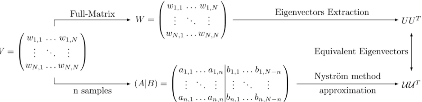
In order to approximate the eigenvectors, we are going to follow the scheme of Figure 3. In this case, we useW, and we take the subsamples setS, which defines a submatrix ofW calledA. These matrices satisfy:
W = ✓
A B BtC
W = 0 B @ w1,1 . . . w1,N .. . . .. ... wN,1. . . wN,N 1 C A W = 0 B @ w1,1 . . . w1,N .. . . .. ... wN,1. . . wN,N 1 C A (A|B) = 0 B @ a1,1. . . a1,nb1,1. . . b1,N n .. . . .. ... ... ... ... an,1. . . an,nbn,1. . . bn,N n 1 C A U UT UUT Full-Matrix n samples Eigenvectors Extraction Nystr¨om method approximation Equivalent Eigenvectors
Figure 3 Eigenvector decomposition applying the Nystr¨om extension. The original Similarity MatrixW is subsampled in the augmented matrix (A|B). Using only this information the Nystr¨om extension is able to approximate the eigenvectorsU ofW as the eigenvectorsU.
Algorithm 4SACOC+Nystrom (SACON) algorithm. Require: X =x1, . . . , xN andknumber of clusters Ensure: c1, . . . , ck bestk clusters
1: Select a subsample of the data instances: S=
{s1, . . . , sn}2X ={x1, . . . , xN}where,n << N.
2: Form the Similarity Graph A2Rn⇥n defined by Aij =e ||si sj||
2
ifi6=j, andAii = 0.
3: Calculate the Matrix B formed by the similarities among the elements of A and the rest of data instances.
4: Calculate the eigenvectors of A, named ¯U and the eigenvalues, named ¯⇤.
5: Calculate the approximate eigenvectors U of W
which try to approximate the real eigenvectors, namedU, as: U = ✓ ¯ U BtU¯⇤¯ 1 ◆
6: Define D to be the diagonal matrix whose (i, i)-element is the sum of thei-th row ofW.
7: Construct the matrixL0=D 1/2W0D 1/2.
8: Separate L0= ✓ A0 B0 (B0)t (B0)t(A0) 1B0 ◆ 9: Set R=A0+ (A0) 1/2B0(B0)t(A0) 1/2, and
calculate its eigenvector decomposition R= UR⇤RURt.
10: SetV=
A0
(B0)t (A0) 1/2UR⇤R1/2.
11: Find v1, . . . , vk, the k largest eigenvectors of L0 and form V = [v1v2. . . vk]2Rn⇥k by stacking the eigenvectors in columns.
12: Form the matrix Y from V by renormalizing each row of V to have unit length (i.e. Yij = Vij/(PjVij2)1/2).
13: ACOC(Y,k).
where A2Rn⇥n, B
2Rn⇥(N n) and C
2
R(N n)⇥(N n)(see line 3 of Algorithm 4). The Nystr¨om Extension will only need the augmented matrix formed by A and B: (A|B). The matrix C is the part that we want to approximate and satisfies that has more elements than A, due ton << N. Using this matrix it
will be able to approximate eigenvectors ofUcalculating the eigenvectors of A, denoted by ¯U (see line 4 of Algorithm 4). These eigenvectors ¯U will be extended to form the approximationU which is close to the original U. Once the eigenvectors ¯U have been calculated, we have the eigendecomposition ofAasA= ¯U⇤¯U¯T because U is orthonormal. Equation 6 provides a methodology to calculateU as (see line 5 of Algorithm 4):
U = ✓ ¯ U BtU¯⇤¯ 1 ◆ (7) which is the approximation of theKfirst eigenvectors of W.
Now, we need to extract the Laplacian eigenvectors, which are extracted from the approximate matrix (see line 7 of Algorithm 4): L0 =D 1/2W0D 1/2, where W0 =U⇤bU, ⇤b= n l⇤¯. Setting Di,i= PN j=1w0i,j we can restructureD as D= ✓ D1 0 0 D2 ◆
where D12Rn⇥n and D22R(N n)⇥(N n) and L can be approximated by (see lines 7 and 8 of Algorithm 4):
L0 = ✓ A0 B0 (B0)t (B0)t(A0) 1B0 ◆ where A0=D 1A and B0 =D2B. In order to approximate the eigenvectors ofL0 we will use the same
methodology that we have used to approximate W- In this case, we are going to use A0 as the base, supposing
that the eigenvectors of A0 and eigenvalues are Vo and
⇤o. ⇤0 =n l⇤ o, V= r l n A0 (B0)t Vo⇤o
where V and ⇤0 are the extended eigenvectors and eigenvalues of L0. Due to V is not orthogonal, which is required by the Spectral Clustering algorithm, we apply the transformation of Fowlkes et al. [9] and defined the matrix (see line 9 of Algorithm 4):
This matrix can be decomposed as R=UR⇤RURt due to A0 is positive define. Then, we set (see line 10 of Algorithm 4): V= A0 (B0)t (A0) 1/2UR⇤R1/2 And, finally, D 1/2W0D 1/2=V⇤RVt
which means thatV are the eigenvectors which will be used for the ACOC clustering algorithm (see line 11 of Algorithm 4).
5 Experimental Setup
The evaluation of the clustering algorithm is a sensitive process, specially when the algorithm deals with large datasets. In this work we have focused the evaluation on comparing the algorithm with other Big Data algorithms. This evaluation has been performed using 8 datasets with 50.000 instances.
The experiments have been carried out using the Nystr¨om extension of Spectral Clustering [9] (SC+N), CluStream, Online K-means and ClusTree.
The parameters of SACON are: the subsample size (fixed to 500), and the sigma value that has been calculated using the methodology described by Ng et al. in [13] (for SC + Nystr¨om is the same); the ants number is 10, the elitism is 1, the exploitation probability is 0.0001, the initial pheromone values have been set to 1/k—wherekis the number of clusters, = 2.0,⇢= 0.1, the local search probability is 0.001 and the maximum number of iterations is 1000.
The metrics used are the Euclidean Distance for online algorithms, and the RBF for the spectral-based algorithms. The evaluation is performed comparing the results with the ideal labels. The evaluation is performed with the accuracy metric, defined by:
sim(Ci, Cj) = Pn q=1 Ci(xq) Cj(xq) 2 ✓ 1 |Ci| + 1 |Cj| ◆ (8) where |Ci| is the number of elements of cluster Ci and
Ci(xq) is the Kronecker defined by:
Ci(xq) =
⇢
0 if xq 2/Ci 1 if xq 2Ci
All the experiments have been executed 100 times. The statistical test which has been performed is the Wilcoxon test, because we can not guarantee that the distributions are normal. It compares SACON with SC+Nystr¨om since these algorithms are very similar to each other. We have considered that there is statistically di↵erence when the p-value of the test is lesser than 0.05 (5% significance level).
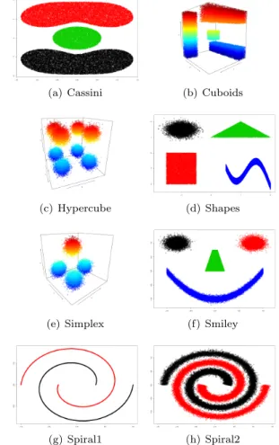
(a) Cassini (b) Cuboids
(c) Hypercube (d) Shapes
(e) Simplex (f) Smiley
(g) Spiral1 (h) Spiral2
Figure 4 The original images of the synthetic datasets
5.1 Dataset Description
The datasets have been generated using the R package mlbench [22] which allows to generate dense datasets with a specific form. The datasets—all composed by 50.000 instances—that have been generated are the following (see Figure 4):
• Cassini: This dataset is formed by 3 clusters which are continuity-based.
• Cuboids: This dataset has four cuboids in three dimensions.
• Hypercube: This datasets is composed by eight spheres distributed as the vertex of a cube.
• Shapes: This dataset has 4 di↵erent shapes.
• Simplex: This dataset has four spheres well separated.
• Smiley: This dataset is formed by four clusters which define a smiley face.
• Spirals1: This dataset has two spirals without noise.
6 Experimental Results
This section presents the evaluation process of SACON. Table 1 shows the results for the algorithms applied to the datasets. As we can appreciate, SACON obtains overall good results, but it is important to analyse the algorithm according to each dataset in order to identify its weaknesses.
In the case of Cassini dataset, SACON obtains the best results. SC+Nystr¨om also obtains good results. It is important to remark that the SD of SACON is 0, which means that these results are stable. The rest of the algorithms obtain worse results. It should be because the dataset (see Figure 4 (a)) has two sections which can be easily defined using a Gaussian distribution, and when the number of instances is high, the boundaries between these distributions are harder for the discrimination process. SC is also sensitive to the noise produced in this situation. The statistical test shows that SACON is significantly better than SC + Nystr¨om.
For Cuboids dataset, Clustream obtains the best Median results (100.0%) followed by SC+Nystr¨om (99.74%). However SACON obtains close results (99.33%). This dataset produces the lesser stable results for SACON (0.0066 of SD), however, the algorithm is the most stable of the algorithms group. These results suggest that the algorithm is also able to deal with volume identification problems (see Figure 4 (b)). The Wilcoxon test shows that there is not statistical di↵erence between the spectral-based algorithms.
Hypercube results show that SACON is able to discriminate the clusters perfectly. Clustream also obtains good results during the discrimination process. SC+Nystr¨om, Clustree and Online K-means have more problems to discriminate the cluster distribution. It might be because the algorithms have to deal with large data quantities and that introduces noise during the calculation (see Figure 4 (c)). The algorithms are also less stable than SACON (the SD of SACON is 0). Again, SACON is significantly better than SC+Nystr¨om approach.
In the case of Shapes, the best results according to the Mean and Median are achieved by Clustream, and the best for Median by Clustree and Online K-means. SACON obtains worse but close results (99.98%) because the algorithm is more stable (the SD is 0.0002). SC+Nystr¨om obtains the worst results of the iteration (68.71%). According to the statistical test, SACON is better again.
Simplexis easy for all algorithms. The Median value shows that they obtain the maximum results. However, according to the Mean, only SACON, Clustream and SC+Nystr¨om keep these results in all the iterations. These results are a consequence of the data structure (see Figure 4 (e)), in this case, they only need to discriminate spheres which is the simplest clustering problem. There is not statistical di↵erence between them.
Smiley results show that SACON obtains the best discrimination results (99.59%). The rest of
the algorithms have more problems generating the clusters. This dataset is a continuity-based problem, therefore only SC+Nystr¨om, Clustream and SACON can discriminate the boundaries (see Figure 4 (f)). SACON is statistically better than SC + Nystr¨om.
The Spiral1dataset tests show how the algorithms can deal with continuity datasets without noise (see Figure 4 (g)). In this case, SACON and SC+Nystr¨om obtain the best results (100.0%). In this case, Online K-means, Clustree and Clustream have more problems discriminating the spirals which means that these algorithms are not able to deal with pure continuity-based problems. There is not statistically di↵erence between them.
TheSpiral2dataset introduces noise to the previous one (see Figure 4 (h)). In this case, the results of SACON are worse than in the previous datasets, but it also obtains the best and more stable results. The results of the rest algorithms show that there is a good minimal solution and all of them are close to this solution (around the 59%), however, they still find problems discriminating the spirals. SACON is significantly better than SC + Nystr¨om.
6.1 Discussion
SACON shows competitive results when it is applied to continuity-based data, such as Cassini, Shapes, Smiley and Spirals while the rest have more problems, e.g., with Spirals which is a pure continuity-based problem. It also performs better than the rest when we add noise to the dataset. The algorithm also obtains more stable results than the others according to the standard deviation. The spectral transformation is probably the main reason of the algorithm improvements. The performance is correlated to the type of clustering that this algorithm can face.
In order to compare the memory usage of the current algorithm against SACOC (its predecessor), it is important to remark that SACON uses a matrix of 50,000⇥500 instances, whereas SACOC uses 50,000⇥
50,000 instances. The memory usage of the former is around 0.18 GB while the latter consumes around 18.63 GB. The memory consume of SACON grows linearly whereas SACOC grows exponentially. The rest of the algorithm are not spectral algorithm, i.e., they do not use a Similarity Matrix. According to the memory consumption, the online algorithms only keep memory about the centroids they are using (similar to K-means), i.e., the memory grows according to the number of centroids, while ACOC keep memory of the assignation of the instance to the centroid, i.e., its memory usage grows linearly according to the product of instances and centroids number.
Dataset SACON SC+Nystrom Online K-means Clustree Clustream Cassini N99.98% ±0.0000 98.61% ±0.1681 65.47% ±0.0003 66.97% ±0.1301 67.39% ±0.0478 Cuboids 99.33%±0.0066 99.74% ±0.1736 88.84% ±0.1219 72.74% ±0.1108 100.0% ±0.1157 Hypercube N100.0% ±0.0000 76.71%±0.1565 81.36% ±0.1122 82.29% ±0.1126 100.0% ±0.0541 Shapes N 99.98%±0.0002 68.71%±0.4425 100.0% ±0.1389 100.0%±0.1765 100.0% ±0.0001 Simplex 100.0% ±0.0000 100.0%±0.0000 100.0% ±0.1508 100.0%±0.1703 100.0% ±0.0000 Smiley N99.56% ±0.0003 74.99%±0.1627 62.54% ±0.1729 64.41% ±0.1608 91.60% ±0.1451 Spirals1 100.0% ±0.0000 100.0%±0.0991 50.00% ±0.0000 50.01% ±0.0002 50.01% ±0.0006 Spirals2 N63.03% ±0.0001 59.59% ±0.0392 59.36% ±0.0000 58.84% ±0.0295 59.59% ±0.0392 Table 1 Median and Standard Deviation accuracy results of the application of the algorithms to the datasets. Values in
bold shows the best results while italics shows the second. TheNsymbol shows those datasets where the results of SACON are statically better than the results of the benchmark algorithm SC + Nystrom.
7 Conclusions
This paper presents an evolution of the SACOC algorithm [5] using the a Nytr¨om extension [9]. The new algorithm, called SACON, applies the spectral transformations and the Nystr¨om extension to the original search space in order to apply the clustering in the projective space. The transformation consists on transforming the original data into a graph-based representation (through a similarity graph) and calculate its Laplacian matrix, during this calculation, the Nystr¨om extension guarantees that the Laplacian calculation is accurate enough using less information. Once the Laplacian has been obtained, the eigenvectors are extracted and normalized to generate the projective space, this extraction also applies the Nystr¨om extension in order to reduce the memory usage.
The proposed SACON algorithm shows good results for the studied datasets. It is able to discriminate continuity-based clusters with more stable results, when compared to Spectral Clustering using the Nystr¨om extension (SC+Nystr¨om) and modern online clustering algorithms.
References
[1] Cheng Chu, Sang Kyun Kim, Yi-An Lin, YuanYuan Yu, Gary Bradski, Andrew Y Ng, and Kunle Olukotun. Map-reduce for machine learning on multicore. Advances in neural information processing systems, 19:281, 2007.
[2] Sudipto Guha, Nina Mishra, Rajeev Motwani, and Liadan O’Callaghan. Clustering data streams. In Foundations of computer science, 2000. proceedings. 41st annual symposium on, pages 359–366. IEEE, 2000.
[3] D. T. Larose. Discovering Knowledge in Data. John Wiley & Sons, 2005.
[4] H´ector D Men´endez, David F Barrero, and David Camacho. A genetic graph-based approach for partitional clustering. International journal of neural systems, 24(03), 2014.
[5] H´ector D Men´endez, Fernando E.B. Otero, and David Camacho. Sacoc: A spectral-based aco clustering algorithm. In Intelligent Distributed Computing VIII, pages 185–194. Springer, 2015. [6] Marco Dorigo and Mauro Birattari. Ant colony
optimization. InEncyclopedia of Machine Learning, pages 36–39. Springer, 2010.
[7] Fernando E.B. Otero, A.A. Freitas, and C.G. Johnson. Inducing decision trees with an ant colony optimization algorithm. Applied Soft Computing, 12(11):3615–3626, 2012.
[8] H´ector D Men´endez, Fernando E.B. Otero, and David Camacho. Macoc: a medoid-based aco clustering algorithm. In Swarm Intelligence, pages 122–133. Springer, 2014.
[9] Charless Fowlkes, Serge Belongie, Fan Chung, and Jitendra Malik. Spectral grouping using the nystrom method. Pattern Analysis and Machine Intelligence, IEEE Transactions on, 26(2):214–225, 2004.
[10] Philipp Kranen, Ira Assent, Corinna Baldauf, and Thomas Seidl. The clustree: indexing micro-clusters for anytime stream mining. Knowledge and information systems, 29(2):249–272, 2011.
[11] Charu C Aggarwal, Jiawei Han, Jianyong Wang, and Philip S Yu. A framework for clustering evolving data streams. In Proceedings of the 29th international conference on Very large data bases-Volume 29, pages 81–92. VLDB Endowment, 2003. [12] Ulrike von Luxburg. A tutorial on spectral clustering. Statistics and Computing, 17(4):395– 416, December 2007.
[13] A. Ng, M. Jordan, and Y. Weiss. On Spectral Clustering: Analysis and an algorithm. In T. Dietterich, S. Becker, and Z. Ghahramani, editors,Advances in Neural Information Processing Systems, pages 849–856. MIT Press, 2001.
[14] Alexandros Karatzoglou, Alex Smola, Kurt Hornik, and Achim Zeileis. kernlab – an S4 package for
kernel methods in R.Journal of Statistical Software, 11(9):1–20, 2004.
[15] Ulrike von Luxburg, Mikhail Belkin, and Olivier Bousquet. Consistency of spectral clustering. The Annals of Statistics, 36(2):555–586, April 2008. [16] Christian Blum and Krzysztof Socha. Training
feed-forward neural networks with ant colony optimization: An application to pattern classification. In Proceedings of the Fifth International Conference on Hybrid Intelligent Systems, HIS ’05, pages 233–238, Washington, DC, USA, 2005. IEEE Computer Society.
[17] Matteo Borrotti and Irene Poli. Na¨ıve bayes ant colony optimization for experimental design. In Rudolf Kruse, Michael R. Berthold, Christian Moewes, Mar´ıa ´Angeles Gil, Przemyslaw Grzegorzewski, and Olgierd Hryniewicz, editors, Synergies of Soft Computing and Statistics for Intelligent Data Analysis, volume 190 of Advances in Intelligent Systems and Computing, pages 489–497. Springer Berlin Heidelberg, 2013.
[18] Yucheng Kao and Kevin Cheng. An aco-based clustering algorithm. In Marco Dorigo, LucaMaria Gambardella, Mauro Birattari, Alcherio Martinoli, Riccardo Poli, and Thomas St¨utzle, editors, Ant Colony Optimization and Swarm Intelligence, volume 4150 ofLecture Notes in Computer Science, pages 340–347. Springer Berlin Heidelberg, 2006. [19] Luca Ashok and David W. Messinger. A spectral
image clustering algorithm based on ant colony optimization. volume 8390, pages 83901P–83901P– 10, 2012.
[20] O.A. Mohamed Jafar and R. Sivakumar. Ant-based clustering algorithms: A brief survey. International Journal of Computer Theory and Engineering, 2:787–796, 2010.
[21] PS Shelokar, Valadi K Jayaraman, and Bhaskar D Kulkarni. An ant colony approach for clustering. Analytica Chimica Acta, 509(2):187–195, 2004. [22] Friedrich Leisch and Evgenia Dimitriadou.mlbench:
Machine Learning Benchmark Problems, 2010. R package version 2.1-1.