Application of deep learning techniques for biomedical data analysis

(1)

Application of Deep Learning Techniques for Biomedical Data

Analysis

A thesis submitted in fulfilment of the requirements for the degree of Doctor of Philosophy

Parham Khojasteh

M. Eng (Shahrood University of Technology) B. Eng (Islamic Azad University, Karaj Branch)

School of Engineering

College of Science, Engineering and Health RMIT University

(2)

i

Declaration of Authorship

I certify that except where due acknowledgement has been made, the work is that of the author alone; the work has not been submitted previously, in whole or in part, to qualify for any other academic award; the content of the thesis is the result of work which has been carried out since the official commencement date of the approved research program; any editorial work, paid or unpaid, carried out by a third party is acknowledged; and, ethics procedures and guidelines have been followed.

Signed: Parham Khojasteh Data: June 2019

(3)

ii

Acknowledgment

I would first like to thank Prof. Dinesh Kant Kumar, who has guided and encouraged me to move During my PhD and has given me immense support as my senior PhD supervisor. I have had the pleasure of working with Dinesh and he has devoted countless hours to my development as a research scientist. Your inspiration, commitment and patience are greatly appreciated.

My thanks go to my associate supervisor Dr. Behzad Aliahmad, who provided support on several successful projects during my PhD.

I would like to thank Dr. João Paulo Papa whom I have worked closely on several projects. With his down-to-earth nature and ability to communicate complex theory, he is a joy to work with.

I would like to offer my thanks to my co-authors, Dr. Sridhar Poosapadi Arjunan, Ms. Rekha Viswanathan, Dr. Leandro Passos, Dr. Tiago Carvalho, Dr. Edmar Rezende. Their expertise and comments were valuable to the papers.

I am grateful to all my friends and colleagues in the Biosignal Lab for their valuable helps and providing inspiring research environment.

Lastly, I would like to thank my family and friends for continual encouragement and support over the last years.

(4)

iii

Publications

1. Khojasteh, P., Aliahmad, B., Kumar, D. (2019) A Novel Color Space of Fundus Images for Reliable Automatic Exudates Detection. “ Journal of Biomedical Signal Processing and Control” 10.1016/j.bspc.2018.12.004

2. Khojasteh, P., Junior, L. A., Carvalho, T., Rezende, E., Aliahmad, B., Papa, J., Kumar, D. (2018) “Exudate detection in fundus images using deeply-learnable features. “Journal of Computers in Biology and Medicine- Elsevier” 10.1016/j.compbiomed.2018.10.031

3. Khojasteh, P., Aliahmad, B., Kumar, D. (2018) Fundus Images Analysis Using Deep Features for Detection of Exudates, Hemorrhages and Microaneurysms. “Journal of BMC Ophthalmology-Springer” 10.1186/s12886-018-0954-4

4. Khojasteh, P., Aliahmad, B., S.P. Arjunan, Kumar, D. (2018) Introducing a Novel Layer in Convolutional Neural Network for Automatic Identification of Diabetic Retinopathy “IEEE EMBC 2018” 10.1109/EMBC.2018.8513606

5. Khojasteh, P., R. Viswanathan., Aliahmad, B., Kumar, D. (2018) Parkinson Disease Diagnosis on Multivariate Deep Features of Speech Signal “IEEE Life Science 2018” 10.1109/LSC.2018.8572136

6. R. Viswanathan, P. Khojasteh, B. Aliahmad, S.P. Arjunan, S. Ragnav, P. Kempster, Kitty Wong, Jennifer Nagao, D. Kumar. (2018) Efficiency of Voice Features Based on Consonant for Detection of Parkinson's Disease. “IEEE Life Science 2018” 10.1109/LSC.2018.8572266

(5)

iv

Abstract

Deep learning and machine learning methods have been used for addressing the problems in the biomedical applications, such as diabetic retinopathy assessment and Parkinson's disease diagnosis. The severity of diabetic retinopathy is estimated by the expert’s examination of fundus images based on the amount and location of three diabetic retinopathy signs (i.e., exudates, hemorrhages, and microaneurysms). An automatic and accurate system for detection of these signs can significantly help clinicians to make the best possible prognosis can result in reducing the risk of vision loss. For Parkinson's disease diagnosis, analysis of a speech voice is considered as the earliest symptom with the advantage of being non-intrusive and suitable for online applications. While some reported outcomes of the developed techniques have shown the good results and ongoing progress for these two applications, designing new algorithms is a thriving research field to overcome the poor sensitivity and specificity of the outcomes as well as the limitations such as dataset size and heuristic selection of the network parameters.

This thesis has comprehensively studied and developed various deep learning frameworks for detection of diabetic retinopathy signs and diagnosis of Parkinson's disease. To improve the performance of the current systems, this work has had an investigation on different techniques: (i) color space investigation, (ii) examination of various deep learning methods, (iii) development of suitable pre/post-processing algorithms and (iv) appropriate selection of deep learning architectures and parameters.

For diabetic retinopathy assessment, this thesis has proposed the new color space as the input for the deep learning models that obtained better replicability compared with the conventional color spaces. This has also shown the pre-trained model can extract more relevant features compared to the models which were trained from scratch. This has also presented a deep learning framework combined with the suitable pre and post-processing algorithms that increased the performance of the system. By investigation different architectures and parameters, the suitable deep learning model has been presented to distinguish between Parkinson's disease and healthy speech signal.

(6)

1

List of Figures

Figure 2.1. Different deep learning models. ... 17

Figure 2.2. A typical CNN architecture (Zhou, Greenspan et al. 2017)... 18

Figure 2.3. Max-Pooling processing on two different feature maps. While the blue matrixes are different, the output are same due to transformation invariance feature. ... 19

Figure 2.4. Comparison of a neural network before and after applying dropout method, where the circles with a cross symbol inside denote deactivated units (Zhou, Greenspan et al. 2017). ... 22

Figure 2.5. AlexNet Architecture (Krizhevsky, Sutskever et al. 2012). ... 23

Figure 2.6. Comparison of the three different topologies used in AlexNet, VGGNet and GoogleNet. ... 24

Figure 2.7. Residual block. (Conv: convolutional layer) ... 25

Figure 2.8. Comparison of the 34-layer residual network with 34-layer plain network and VGG-19 (He, Zhang et al. 2016). ... 26

Figure 2.9. U-net architecture for segmentation application (Ronneberger, Fischer et al. 2015). ... 28

Figure 2.10. The architecture of multiscale three-layer neural network (Zhao and Jia 2016). ... 29

Figure 2.11. Transfer learning process (Tan, Sun et al. 2018). ... 31

Figure 2.12. An example of the RBM architecture. ... 33

Figure 3.1.Schematic of PCA transformation procedure on an image. ... 44

Figure 3.2. Samples from DIARETDB1 database: (a) Image from a patient where exudates are highlighted in blue, and (b) Image from a healthy subject without any exudate. ... 47

Figure 3.3. Eigenchannels of RGB, HSI and LUV: (a) Original RGB image; (b) 1st Eigenchannel of RGB; (c) 2nd Eigenchannel of RGB; (d) 3rd Eigenchannel of RGB; (e) 1st Eigenchannel of HSI; (f) 2nd Eigenchannel of HSI; (g) 3rd Eigenchannel of HSI; (h) 1st Eigenchannel of LUV; (i) 2nd Eigenchannel of LUV; (j) 3rd Eigenchannel of LUV. ... 49

Figure 3.4. Examples of Exudate patches. ... 50

(11)

6

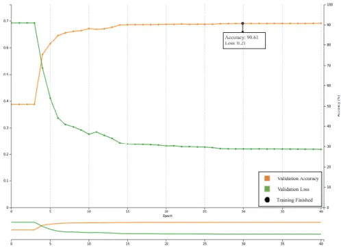
Figure 3.6. Accuracy and loss values over 40 training epochs for the RGB space. A

saturation can be observed after the 30th epoch. ... 52

Figure 3.7. SSIM index between channels of HSI and PCA-RGB spaces. ... 54

Figure 3.8. Comparing replicability of the three spaces (PHS, HSI and PCA-RGB) using 20-fold cross validation approach with 20 runs. ... 55

Figure 3.9. Variation of the accuracy changes for the three spaces (PHS, HSI and PCA-RGB) using 20-fold cross-validation approach with 20 runs. ... 55

Figure 3.10. Distribution of the exudate and background pixels of an exudate patch sample in different color spaces. ... 57

Figure 4.1. Architecture of the proposed CNN used in this work. ... 63

Figure 4.3. Samples of exudate patches ... 66

Figure 4.6. Flowchart for detecting exudate and non-exudate patches. ... 67

Figure 4.7. Accuracy and loss changes over 40 training epochs concerning the DIARETDB1 database. A saturation is observed after the 30th epoch. ... 68

Figure 4.8. Heat map obtained from the grid-search showing the best combination of learning rate and the number of hidden units. ... 69

Figure 4.9. Change of accuracy of the network corresponding to different learning rates. 74 Figure 5.1. Architecture of the proposed CNN- I: input image, PPL: pre-processing layer C: convolutional layer, FP: feature map, MP: max pooling, FC: fully-connected layer. ... 79

Figure 5.2. Patch examples corresponding to four classes: (a) exudate; (b) hemorrhage; (c) microaneurysm; (d) background... 80

Figure 5.3. The training process for three designed CNNs. After 53, 65 and 74 epochs, the training process stopped for CE, CLAHE and No-PPL, respectively. ... 82

Figure 5.4. Total accuracy of the classification corresponding to three CNNs. ... 84

Figure 6.1. Example of Retina Images containing three DR sings. This image shows an entire retina image with haemorrhage, microaneurysm and exudate labelled by graders, and which was then cropped to illustrate individual patch. ... 87 Figure 6.2. Overview of the proposed framework contains two main phases: 1) patch-based and 2) image-based analysis. The patch-based section corresponds to training and testing a

(12)

7

CNN model to discriminate between the different DR signs. Image-based analysis of the entire image generates probability maps for each sign. ... 93 Figure 6.3. Applying the image enhancement technique on an example retina image. (a) Original retina image; (b) After image enhancement. This shows that some new lesions can be singularized by image enhancement shown by yellow annotations). ... 94 Figure 6.4. Process of generating three probability maps corresponding to exudate, hemorrhage and microaneurysm from a retina image. By taking a patch of size S×S centered around pixel (𝑥𝑖, 𝑦𝑖), each patch is fed to the trained CNN that determines the membership probabilities at location 𝑥𝑖, 𝑦𝑖 for the three pathological signs: i.e. exudate, hemorrhage and microaneurysm (shown by PE,xi,yi, PH,xi,yi and PM,xi,yi). ... 95 Figure 6.5. Patch examples corresponding to the four classes; (a) exudate. (b) hemorrhage. (c) microaneurysm. (d) no-sign. ... 97 Figure 6.6. Three probability maps were generated from an example retina image: (a) original retina image; (b) Exudate probability map; (c) Hemorrhage probability map; (d) Microaneurysm probability map. Colorbar shows the severity level of a pixel belong to the sign that is ranging between 0 to 1 corresponding to blue to red color. ... 98 Figure 6.7. Three examples of pathological signs before and after post-processing. (a) Original image. (b) Probability map corresponding to the sign. (c) Image output after post-processing ... 99 Figure 6.8. ROC curve corresponding classification of the four classes (exudate, hemorrhage, microaneurysm and no-sign). This shows that the CNN-model obtained the highest AUC for detection of exudate (yellow color) and almost same AUC for detection hemorrhage and microaneurysm. ... 100 Figure 6.9. Performance of proposed framework for the sign detections using two databases (DIARETDB1 and e-Ophtha) compared to the method with binary outputs of the network. ... 101 Figure 6.10. Segmentation output image of the example retina image. (a) Manually annotated images that exudate, hemorrhage, and microaneurysm signs marked by blue, green and pink color, respectively. (b) Segmented output by the proposed algorithm. ... 101 Figure 7.1. Overview of the proposed framework. ... 108

(13)

8

Figure 7.2. Performance of the proposed networks corresponding to different frame sizes: (a) Accuracy (b) PPV (c) Sensitivity (d) Specificity. ... 112

(14)

9

List of Tables

Table 2.1. Detail of the different architectures used in (Mazo, Bernal et al. 2018). ... 32 Table 3.1. Architecture of the proposed CNN. I - Input image, C - Convolutional layer, MP - Max pooling layer, FC - fully-connected, FM - Feature map, CH - Channels, Neurons-N. ... 46 Table 3.2. CNN parameters for train and test phases. ... 51 Table 3.3. Performance of the six spaces for the detection of the exudates. ... 53 Table 3.4. Changes of Dµ and DΣ from a color space to transformed orthogonal space (↑ = increase, ↓ = decrease). ... 57 Table 3.5. Comparison the result of proposed method with previous works reported in the literature. The symbol ‘-‘ stands for unreported results. DR1 and EO corresponding to DIARETDB1 and e-Ophtha databases, respectively. ... 59 Table 4.1. Performance of the proposed methods for DIARETDB1 database: overall accuracy, sensitivity, and specificity. ... 70 Table 4.2. Performance of the proposed methods for e-Ophtha database: overall accuracy, sensitivity, and specificity. ... 70 Table 4.3. Comparison of the proposed approach against other works reported in the literature. The symbol `-' stands for unreported results. ... 72 Table 5.1. Statistics of the patches- exudate (EX), hemorrhage (HM), microaneurysm (MA) and background (BK). ... 81 Table 5.2. Performance of three proposed CNNs- exudate (EX), hemorrhage (HM), microaneurysm (MA) and background (BK). ... 83 Table 6.1. Comparison between performance of the pervious methods for detection of exudate, hemorrhage and microaneurysm. ... 89 Table 6.2. Validation parameters ... 96 Table 6.3. Statistics information of sign patches. ... 97 Table 6.4. Sensitivity, specificity, accuracy and PPV of the proposed method in patch-level evaluation for detection of exudate, hemorrhage and microaneurysm... 99

(15)

10

Table 7.1. Proposed DCNN’s architectures. Conv (𝑎 × 𝑏 × 𝑐): convolutional layer with 𝑎

feature maps and size of 𝑏 × 𝑐 pixels, MP (𝑒 × 𝑓) : max-pooling layer with kernel size of

𝑒 × 𝑓 pixels, FC (𝑛): fully connected layer with 𝑛 neurons... 109 Table 7.2. Statistics of frames using different window seizes in training, validation and test sets. ... 110

(16)

11

Chapter 1

1

Introduction

1.1

Introduction

A combination of machine learning, image and signal processing methods have been used to address various problems in the biomedical applications, such as Diabetic Retinopathy (DR) assessment and Parkinson’s Disease (PD) diagnosis (Kahai, Namuduri et al. 2006, Rahn, Chou et al. 2007, Lee, Zhou et al. 2008, Gracas, Gama et al. 2012, Zaki, Zulkifley et al. 2016). Unlike the conventional pipeline that required hand-crafted feature extraction, Deep Learning (DL) methods have overcome this issue by automatically learning informative features from the input data (Schmidhuber 2015, van Grinsven, Venhuizen et al. 2016, Kamal Maried, Abdalla Eldali et al. 2017, Tan, Fujita et al. 2017). Achieving the promising results in different applications by the DL methods has led to increasing a demand for developing new DL techniques to improve the performance of the current systems. This thesis has investigated to develop novel DL frameworks for two biomedical applications:

• DR Assessment

• PD Diagnosis

Diabetic Retinopathy Assessment. The severity of DR is currently estimated by the expert’s

examination of fundus images based on the amount and location of three retinopathy signs (i.e., exudates, hemorrhages, and microaneurysms) across the retina surface (Hansen, Abramoff et al. 2015). If the DR severity is misdiagnosed, it can lead to irreversible vision loss (Mohamed, Gillies et al. 2007, Shaw, Sicree et al. 2010). Consequently, an automatic and accurate system for detection of the DR signs can significantly help clinicians to make the best possible prognosis about the severity of DR and risk of vision loss. For this purpose,

(17)

12

DL and other machine learning methods have been employed (Hajeb Mohammad Alipour, Rabbani et al. 2012, Lazar and Hajdu 2013, Tang, Niemeijer et al. 2013).

Parkinson’s Disease Diagnosis. The speech impairment in PD, as one of the earliest

symptoms, has been considered for the diagnosis of the disease. It has the advantage of being non-intrusive and suitable for online applications, and hence researchers have investigated the speech features to diagnose PD (Tsanas, Little et al. 2010, Zhang, Yang et al. 2016, Pompili, Abad et al. 2017). Machine learning and speech processing techniques have been utilized to analyse the speech signals to classify between PD and control subjects.

1.2

Problem Statement

Among the three DR signs, the presence of exudate is observed as the earliest sign of DR. For automatic exudate detection, various DL and machine learning methods have been developed. However, the current methods have some drawbacks described as follow.

• Retina image analyses have been conducted using color spaces such as RGB, HSV, and LUV. Majority of the DL methods use three channels of the RGB space as the input to the networks (Gargeya and Leng 2017, Quellec, Charrière et al. 2017, Grassmann, Mengelkamp et al. 2018). However, other color spaces haven’t been explored and tested with DL methods.

• Most of pervious DL frameworks are based on the Convolutional Neural Networks (CNNs) architecture. This requires identifying the suitable architecture and optimal parameters. However, there is no exact method for the selection of the network parameters (He, Zhang et al. 2016).

• Another concern in using the CNN-based methods is the need for a large dataset to train the CNN. For overcoming these limitations, there is a need to investigate different DL methods to identify a network that gives good performance and is not reliant on large datasets.

(18)

13

The success of diagnosis of DR requires the detection of all the three signs: exudate, hemorrhage and microaneurysm. For the simultaneous detection of all DR signs, a few studies have been conducted by employing the CNN-based methods, but their methods achieved poor performance for distinguishing between hemorrhage and microaneurysm (Tan, Fujita et al. 2017). One of the main drawbacks in these works is not using the suitable DL-based framework with appropriate pre/pro-processing methods in their algorithm. It is observed that pre-processing methods have significant effect on enhancing the contrast between the DR signs and backgrounds. Although various pre-processing techniques have been developed for the DR assessment, comparing the performance of these methods have not been tested for the DL-based methods. Additionally, the effect of post-processing methods on the output of these methods have not been investigated for automatic DR signs detection. As a result, it is essential to investigate various pre/pre-processing methods to find the suitable one for improving the performance of the CNN-based methods.

For PD diagnosis based on the speech signal, many studies have attempted to extract and analysis the time-frequency-based features, such as Jitter, Shimmer, Pitch, Harmonics to Noise Ratio, Autocorrelation, voiced and unvoiced frames (Sakar, Isenkul et al. 2013). However, there is the need for improving the performance for diagnosis. This aim of this sub-section was to investigate CNN-based models can provide informative features while the efficiency of such these models have not been tested yet.

1.3

Hypotheses

This thesis aims to investigate and develop different DL methods for assessment of DR and PD. This research has been conducted based on the following hypothesis:

i. An appropriate choice of color channels is expected to enhance the performance of the system for automatic DR signs detection.

ii. Identify a suitable DL method is able to overcome the limitations of the CNN-based methods for automatic DR signs detection.

iii. A combination of suitable pre/post-processing algorithms is expected to increase the performance of the DL-based method for automatic DR signs detection.

(19)

14

iv. DL methods are able to extract suitable informative features from the speech signals for distinguishing between PD and healthy individual.

1.4

Research Aim and Objectives

The aim of this research is to study and investigate the use of DL for two biomedical applications: (i)- retinal image analysis for DR assessment and (ii)- for speech analysis for PD diagnosis. The objectives of this research are to:

i. Develop a framework of DL for detection and segmentation of DR signs in the color fundus images.

ii. Investigate and compare different color spaces of fundus images for DR signs detection

iii. Compare different DL methods (CNN, pre-trained and Restricted Boltzmann Machine (RBM) models) for detecting the DR signs.

iv. Investigate different image enhancement methods to improve the performance of DL-based techniques.

v. Develop a post-processing algorithm to improve the performance of DL-based techniques.

vi. Develop a DL model for automatic and simultaneous detection of three DR signs. vii. Propose a DL model for assessment of PD using speech signal.

viii. Investigate various DL architectures to identify suitable architecture for PD assessment.

This research has comprehensively studied and developed various DL methods for detection of DR signs and diagnosis of PD. This demonstrates the importance of combining the machine learning, image and signal processing techniques to the DL techniques and assess the impact of them on the clinical applications. This also suggests using suitable color channels and DL’s architecture combined with appropriate pre/post processing algorithms can have a significant impact on the performance of the system. This thesis also delivers the effect of different designs of DL architectures on the system’s performance.

(20)

15

1.5

Outline of the Thesis

The chapters of the thesis are organized as follow:

Chapter 1 describes the overall thesis with an introduction, problem statement, hypothesis

and aims, and objectives of the work.

Chapter 2 presents a literature review of the DL methods used in this thesis.

Chapter 3 investigates and compares the performance of different color spaces of fundus

images for automatic detection of exudates.

Chapter 4 investigates different DL techniques to maximize the sensitivity and specificity

of the method for automatic detection of exudates.

Chapter 5 proposes a novel pre-processing layer in the CNN architecture to increase the

performance of the system for DR signs detection.

Chapter 6 develops a method using the probabilistic output of the CNN model to

automatically and simultaneously detect the DR signs.

Chapter 7 investigates the efficiency of the CNN model in distinguishing between

Parkinson’s and healthy voices.

Chapter 8 concludes the findings of the thesis and discusses future studies to be

(21)

16

Chapter 2

2

Methodology Background

2.1

Overview

This chapter provides a literature review of the fundamentals of DL with a focus on the methods used in this thesis. It also provides a description of the software and hardware that is required for implementation of the algorithms. This introduces the fundamental concepts of the DL methods and comparison of their performances in the different applications of biomedical data analysis.

2.2

Deep Learning Algorithms

In common machine learning pipelines for different applications, extracting informative features are conducted by the machine learning experts on the basis of their knowledge about the target domain (Shen, Wu et al. 2017). However, DL methods have overcome this issue by learning a hierarchy of features from input data (Schmidhuber 2015, Kamal Maried, Abdalla Eldali et al. 2017). Instead of a handy-crated feature selection and extraction, the DL methods automatically learn the informative representation in a self-taught manner (LeCun, Bengio et al. 2015).

Researches have become interested in using DL methods because these methods not only require less engineering efforts but also have achieved record-breaking performances in the variety of artificial intelligence applications (Collobert and Weston 2008, Mikolov, Deoras et al. 2011, Sutskever, Martens et al. 2011, Hinton, Deng et al. 2012, Krizhevsky, Sutskever et al. 2012, Farabet, Couprie et al. 2013, Sainath, Mohamed et al. 2013, Tompson, Jain et al. 2014, Suk and Shen 2015, Szegedy, Wei et al. 2015, Zhang, Li et al. 2015, Kleesiek, Urban et al. 2016, Wu, Kim et al. 2016).

(22)

17

DL methods, generally, can be categorized into the five main groups (shown in Figure 2.1):

• CNNs

• Pre-trained models

• Deep neural networks (Auto-Encoders)

• Deep generative models (Restricted Boltzmann Machines (RBMs))

• Sequential models (Recurrent Neural Networks (RNNs))

Figure 2.1. Different deep learning models.

In this thesis, three DL methods are used and described in this section:

• CNNs

• Pre-trained Models

• RBMs

2.2.1

Convolutional Neural Network

CNN architectures and their applications are explained as folow.

Deep Learning Convolutional Neural Network Pre-trained Model Deep Neural Network Deep Generative Model Sequential Model

(23)

18

2.2.1.1 Convolutional Neural Network’s Architecture

A CNN architecture, basically, is comprised of different layers including convolutional and pooling (down-sampling) layers that are followed by fully connected layers (similar to multi-layer neural networks). A typical CNN architecture is shown in Figure 2.2.

Figure 2.2. A typical CNN architecture (Zhou, Greenspan et al. 2017).

Convolutional layer

The purpose of the convolutional layer is to detect local features at different positions of the feature map of the pervious layer where a feature map is the output of one filter applied to the pervious layer. According to formula (2.1), each neuron from the same convolutional matrix generates 𝑛 feature maps in the convolutional layer if there are 𝑛 kernels.

𝐴𝑖 = 𝑓 (∑ 𝐼𝑗∗ 𝐾𝑖 + 𝐵𝑗 𝑁

𝑗=1

) (2.1)

In formula (2.1), 𝐼_𝑗 is 𝑗th_{input matrix, where there is only one input matrix from the input} layer, and 𝑓(. ) is a nonlinear activation function. 𝑘_𝑖, 𝐵_𝑖, ∗ indicate the 𝑖th_{convolutional} kernel matrix, bias matrix and a convolutional operation, respectively.

Pooling Layer

A pooling layer follows the convolutional layer to downsample and reduce the size of the feature map of the preceding convolution layer. This layer is responsible to progressively

(24)

19

reduce the spatial size of the feature map and decrease the number of computations and parameters. Another advantage of pooling layer is for transformation invariance over small spatial shifts in the input. Among different types of the pooling layers, Max-Pooling is the most privilege method which is widely used in the CNN’s architectures. This layer selects the maximum number of each stride. Figure 2.3 shows an example of the transformation invariance feature of the Max-Pooling operation on the two different feature maps. While the blue matrix by the size of 2×2 in the feature maps is different, the output for both are same because the blue matrix in feature map B is the horizontally flipped version of the feature map A.

Figure 2.3. Max-Pooling processing on two different feature maps. While the blue matrixes are different, the output are same due to transformation invariance feature.

Fully Connected layer

Fully connected layers have the characteristic as same as the multi-layer neural networks (Abbod, Catto et al. 2007, van Gerven and Bohte 2017). The input units are the last proceeding feature map which is reshaped to a vector followed by the hidden layers and the output units are mostly the number of target classes which varies from one application to another one.

(25)

20

In a CNN architecture, updating learnable parameters (weights and biases) require a training phase which is described as follow.

Training Convolutional Neural Networks

To train a CNN model, the back-propagation algorithm is used to update the network parameters (weights and biases). Assuming that 𝜃 = {𝑊_𝑖, 𝑏_𝑖} defined as network parameters, where 𝑤 and 𝑏 correspond to weight and bias in the convolutional and fully connected layers, respectively. For the training process, the loss function of 𝐿_𝑐 is defined as follow: 𝐿𝑐 = − 1 |𝐶| ∑ ln (𝑝(𝐷 𝑖_|𝐶𝑖₎₎ |𝐶| 𝑖=1 (2.2) Where |𝐶| represents the number of items in the training data, 𝐶𝑖_and_𝐷𝑖 _{denote the}_ith

training sample and its label, respectively. To update 𝜃 parameters, stochastic gradient descent (SGD) (Pang, Yu et al. 2017) method is used. The 𝜃 in each iteration is updated by (2.3):

θ(p + 1) = θ(p) − γ∂Lc

∂θ + ∆θ(p) − µγθ(p) (2.3)

where γ, ϑ and µ denote learning rate, momentum rate and weight delay rate, respectively. One of the main challenges in training a deep CNN architecture is the backpropagated error message that becomes inefficient due to vanishing gradient after repeated multiplications which is called ‘Vanishing Gradient’ (Schmidhuber 1992). This causes the slower learning process in the layers close to the input layer compared to ones are closer to the output layer. To tackle this issue, some techniques are proposed as follow:

• Rectified Linear Unit

• Batch Normalization

(26)

21

Rectified Linear Unit

A neuron activation function is a step after the convolutional and fully connected layer. In the multi-layer neural networks, the hyperbolic tangent and sigmoid are the two most common non-linear activation functions methods which are used. Using such these functions, however, lead to decreasing the classification accuracy in the deep CNNs because of the saturation characteristics which could make the output gradient drop close to zero (Li, Cai et al. 2014). To address this issue, non-linear non-saturating functions, such as Rectified Linear Unit (RELU) and maxout (Goodfellow, Warde-Farley et al. 2013) functions, are used in the CNN architectures. The RELU function can vanish the gradient problem (Hinton and Salakhutdinov 2006, Glorot and Bengio 2010), and consequently, leads to improving the learning speed. The RELU is given by formula (2.4).

𝐹(𝑥) = max(0, 𝑥) (2.4)

Batch Normalization

Due to the change in the network parameters during the training phase, it’s observed that the change in the distribution of the network activations could cause longer training time. To address this problem, Ioffe and Szegedy (Ioffe and Szegedy 2015) presented a batch normalization method by applying the normalization for each mini-batch and backpropagating the gradients through the normalization parameters such as scale and shift. This layer follows the Max-Pooling layer to refine the pooling layer. Each unit of feature map is normalized by 2.5 :

𝑢̂_𝑖 = 𝑢𝑖− Ē[𝑢𝑖]

√𝑉𝑎𝑟 [𝑢_𝑖] (2.5)

Where 𝑖 stands for an index of the units (𝑢_𝑖) in the layer. In the next step, a pair of learnable parameters 𝛼_𝑖 and 𝛽_𝑖 are introduced to scale and shift the normalized values as follow:

(27)

22

The output of equation 2.6 (𝑦𝑖) then is fed into the following layer.

Dropout

The aim of dropout technique is to randomly deactivate a fraction of the units, e.g., 50%, in a network on each training iteration. This method prevents a complex co-adaptation among units that helps the CNN to avoid overfitting. The temporal and random removal of unites in the training phase can be assumed to train the different networks with sharing connections weights. This method is used in the training phase, while all units must be activated in the test phase. Figure 2.4 shows a neural network before and after applying the dropout, where the circles with a cross symbol inside denote deactivated units.

Figure 2.4. Comparison of a neural network before and after applying dropout method, where the circles with a cross symbol inside denote deactivated units (Zhou, Greenspan et al. 2017).

2.2.1.2 Application of Convolutional Neural Networks

Different CNN architectures and number of parameters have resulted in presenting various networks used in addressing different problems. The main CNN’s applications can be categized into:

• Image classification, segmentation and registration

• Object detection

• Speech analysis

• Text detection and recognition

(28)

23

In this thesis, image classification and segmentation and speech analysis are used.

Image Classification

In 1990, the first version of the CNN model was introduced by LeCun et al. for hand-written digits recognition (Cun, Boser et al. 1990). The main purpose of this network (LetNet) was to classify handwritten digits into the ten classes. LetNet with five layers could not achieve a promising result due to the lack of a large number of data sets for training the model. In 2012, Krizhevsky et al. (Krizhevsky, Sutskever et al. 2012) presented the ‘AlexNet’ with eight layers including five convolutional and pooling layers and three fully connected layers (shown in Figure 2.5) which won the completion of ImageNet challenge (Russakovsky, Deng et al. 2015) and attracted lots of attention from the other researchers in machine learning and computer vision field.

Figure 2.5. AlexNet Architecture (Krizhevsky, Sutskever et al. 2012).

The results of the AlexNet showed a decent accuracy although training these numbers of weights took lots of time. For addressing this issue, the ability of graphical processing units (GPUs) for parallel processing were used to decrease the training time while it took a long time just by using central processing units (CPUs). Currently, both GUPs and CUPs are managed to do some parts of the process together. By using smaller kernel size in the convolutional layer, a similar function can be represented with fewer parameters. Another advantage of such networks is having a lower memory footprint which makes a reliable and feasible deployment of these models on some devices such as esdge devices. In 2014,

(29)

24

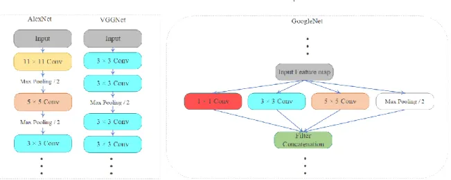
Simonyan and Zisserman (Simonyan and Zisserman 2014) proposed a CNN architecture ( VGGNet ) with 19 layers that won the ImageNet challenge of 2014. Presenting the deeper models continued until ‘GoogleNet’ was proposed by Szegedy et al. (Szegedy, Liu et al. 2014). Beside using deeper architecture, this model introduced inception blocks (Lin, Chen et al. 2013). Unlike the previous networks (AlexNet and VGGNet), the inception block in GoogleNet extracts features with the different kernel sizes in the inception block that then they are concatenated at the end of the inception block. Comparison of different topologies used in AlexNet and VGGNet with GoogleNet are shown in Figure 2.6. This image shows that the AlexNet employs different kernel sizes (11×11, 5×5 and 3×3) and VGGNet uses the small kernel size (3×3). However, GoogleNet utilizes the inception module was able to extract features by different kernel sizes.

Figure 2.6. Comparison of the three different topologies used in AlexNet, VGGNet and GoogleNet.

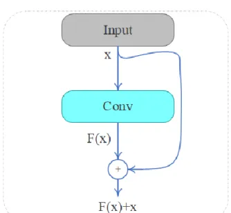
After presenting GoogleNet, the researchers tried to develop a deeper network to increase the performance of the system. However, it was observed that increasing the number of layers was led to decreasing the accuracy due to the vanishing gradient problem that even was not compensated even by using the RELU and dropout layers. In 2015, the solution was devised by He et al. (He, Zhang et al. 2016) by introducing residual connections (He, Zhang et al. 2016). In the residual setup, this does not only pass the output of convolutional layer (F(x)) to the next layer, but this also adds up the input of convolutional layer (x) and then

(30)

25

pass (F(x) + x) to the next layer (Figure 2.7). Expanding this principle into the entire network resulted in introducing the new architecture ‘ResNet’ that won ImageNet completion in 2015.

Figure 2.7. Residual block. (Conv: convolutional layer)

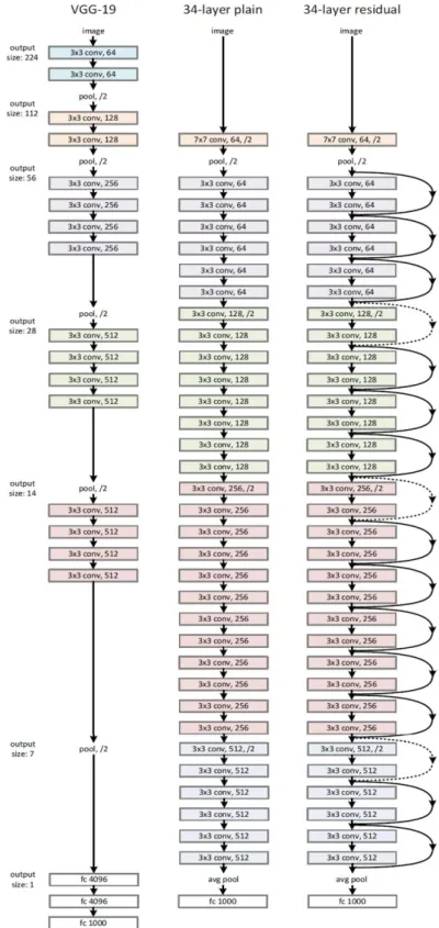
In Figure 2.8, the 34-layer residual network is compared with 34-layer plain network and VGG-19.

(31)

26

Figure 2.8. Comparison of the 34-layer residual network with 34-layer plain network and VGG-19 (He, Zhang et al. 2016).

(32)

27

Image Segmentation

One of the drawback of using a fully convolutional neural network (fCNN) for the segmentation of the entire image is losing resolutions due to the pooling layers. ‘Shift-and-stitch’ is one of the several techniques proposed to prevent this resolution decrease (Shelhamer, Long et al. 2017). The fCNN was applied to a shifted version of the input image and by stitching the result together, one obtains a full resolution version of the final output, minus the pixels lost due to the ‘valid’ convolutions.

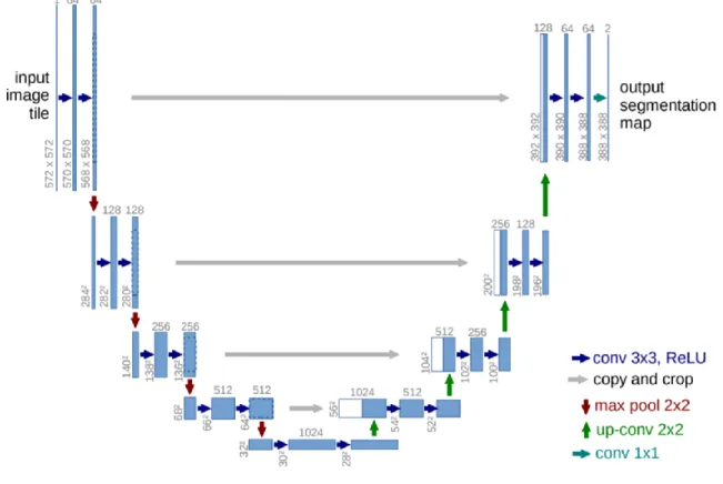
Using an upsampling path was become popular among the proposed CNN-based methods for the segmentation purpose (Long, Shelhamer et al. 2015). In 2015, Ronneberger et al. (Ronneberger, Fischer et al. 2015) proposed ‘U-net’ architecture comprising a fCNN followed by an upsampling section which increased the image size (shown in Figure 2.9). The authors combined it with skip-connections to directly connect opposing expanding and contracting convolutional layers. Milletari et al. (Milletari, Navab et al. 2016) extended this U-Net layout that incorporates ResNet and a Dice loss layer that could directly minimize segmentation error.

(33)

28

Figure 2.9. U-net architecture for segmentation application (Ronneberger, Fischer et al. 2015).

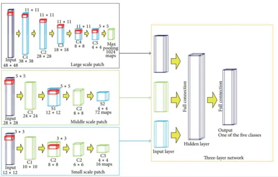
As another example of a CNN-based model for segmentation purpose, mitosis detection for screening the breast cancer was one the first work in this area (Ciresan, Giusti et al. 2013). For pixel classification, they used ‘sliding-window’ approach that each pixel was presented by the neighborhood pixels. The developed CNN architecture could win the ICPR competition in 2012. However, a drawback of this naïve method is producing huge overlaps for analyzing the pixels as well as variability of the window sizes. Small patches can introduce just local information of the image while the larger ones are the presenter of global characteristics. However, both local and global features can play an important role in some applications (Shyu, Brodley et al. 1998, Murphy, Torralba et al. 2006). To address this issue, Zho and Jia (Zhao and Jia 2016) proposed a multiscale CNN model for brain tumor segmentation. Instead of one fixed patch size, they trained three networks with the three different patch sizes (48×48, 28×28 and 12×12) and the output was yielded by a

(34)

29

combination of the three networks (Figure 2.10). In comparison to the traditional one-pathway architecture, their algorithm was more accurate and robust.

Figure 2.10. The architecture of multiscale three-layer neural network (Zhao and Jia 2016).

As a segmentation application of the CNN-based method for retinal image analysis, Li et al. (Li, Feng et al. 2016) turned the segmentation task into vessel mapping problem by using a 5-layer deep neural network for segmentation of the vessels in retinal fundus images. In 2016, Liskowski and Krawiec (Liskowski and Krawiec 2016) proposed a structure prediction scheme to highlight the context information with a 7-layers CNN architecture without any pooling layer. Similarly, Fu et al. (Fu, Xu et al. 2016) with a combination of the 7-layer CNN and conditional random field presented a recurrent neural network to model long-range pixel interactions. In 2018, a combination of the wavelet transform with a CNN model was presented to overcome the variability of width and direction of the vessel structure in the retina (Oliveira, Pereira et al. 2018). As a result of features of CNN-based model described above, the main advantages and drawbacks of these models can be concluded as follow (Pak and Kim 2017, Batmaz, Yurekli et al. 2018, Khan and Yairi 2018, Nash, Drummond et al. 2018).

(35)

30 Advantages:

• State-of-the-art performance in a variety of applications.

• Automatically salient features extraction from different types of data.

• The ability to perform function operation rapidly on multiple core GPUs up to 5000% over CPU-only implementations.

Drawbacks:

• Require large datasets to train the model from scratch (small dataset could just train the limited number of the neurons which not reflecting the high-level representations).

• Evaluating and tuning lots of parameters in order to get high performance, such as number of the layers, kernel size, filters, learning rate and type of activation function.

2.2.2

Pre-trained Model

As mentioned in section 2.2.1.2, training a CNN model from scratch requires a large dataset. However, most of the medical datasets are typically small ( hundreds/thousands of samples) compared to millions of images in the computer vision application (Russakovsky, Deng et al. 2015). Therefore, using pre-trained models (Transfer Learning) has become popular among the researchers, especially in medical image applications.

Transfer learning is a method that transfer the knowledge from the source domain to the target domain (Figure 2.11).

(36)

31

Figure 2.11. Transfer learning process (Tan, Sun et al. 2018).

There are two strategies for transfer learning:

• Using a pre-trained network as a feature extractor

• Fine-tuning a pre-trained network

Compare to the fine-tunning method, the extra benefit of using a pre-trained network as a feature extractor is not requiring a training stage and tunning network’s parameters that is easily plugged into the existing image analysis pipelines. To compare the performance of these two strategies, different studies were investigated (Azizpour, Razavian et al. 2015, Gulshan, Peng et al. 2016, Kim, Corte-Real et al. 2016, Tajbakhsh, Shin et al. 2016, Esteva, Kuprel et al. 2017, Tiulpin, Thevenot et al. 2018). For instance, Li et al. (Li, Pang et al. 2017) used three different approaches for classification of DR: (i) find-tunning, (ii) transfer learning and (iii) full training. Their results showed that the transfer learning method outperformed the other approaches.

For different applications, different pre-trained models were used. For classification of tissues in histological images, Mazo et al. (Mazo, Bernal et al. 2018) used four different pre-trained models (VGG-16, VGG-19, GoogleNet and ResNet) which initially pre-trained on the ImageNet dataset (Russakovsky, Deng et al. 2015). It is worth to mention that each network has a different architecture with a different number of parameters (Table 2.1).

(37)

32

Table 2.1. Detail of the different architectures used in (Mazo, Bernal et al. 2018).

Item VGG-16 VGG-19 GoogleNet ResNet

General Parameters 15.5 M 20.8 M 24.1 M 25.9 M Channels 3 3 3 3 Input size 100×100 100×100 150×150 200×200 Number of layers Convolutional 13 16 94 53 Max- Pooling 5 5 4 1 Fully connected 3 3 3 3 Presence of modules

Batch normalization No No Yes Yes

Residual connection No No No Yes

Abbasi-Sureshjani et al. (Abbasi-Sureshjani, Dashtbozorg et al. 2018) used the ResNet architecture for extracting a feature from retinal fundus images for DR assessment.

It can be seen that different pre-trained models have been used in different applications. Therefore, the success of the transfer learning method (either fixed feature extractor or fine-tuning) is subjected to the application and the type of network.

2.2.3

Restricted Boltzmann Machine

The first version of the Restricted Boltzmann Machine (RBM) models was presented by Smolensky in 1986 (Smolensky 1986) and it was then represented based on the fast learning algorithm by Hinton (Hinton 2012). An RBM model is an unsupervised method and energy-based stochastic neural networks composed of two different layers: (i) Visible layer and (ii) Hidden layer. These layers include a different number of visible (𝑉) and hidden (ℎ) units,

(38)

33

respectively. A weight matrix (𝑊𝑚×𝑛) stands for the connection weights between the visible

and hidden layer with 𝑚 and 𝑛 units, respectively. This connection is bidirectional, so given an input vector 𝑉 that one can obtain the latent feature representation ℎ and vice versa (Figure 2.12)

Figure 2.12. An example of the RBM architecture.

An energy function of 𝐸(𝑣, ℎ) is defined and minimized by:

𝐸(𝑣, ℎ) = − ∑ 𝑎𝑖𝑣𝑖 𝑚 𝑖=1 − ∑ 𝑏𝑗ℎ𝑗 𝑛 𝑗=1 − ∑ ∑ 𝑣𝑖ℎ𝑗𝑊𝑖𝑗 𝑛 𝑗=1 𝑚 𝑖=1 (2.7)

Where 𝑎 and 𝑏 are the biases of visible and hidden unites, respectively. The probability of joint configuration (𝑣, ℎ) is computed as follow:

𝑃(𝑣, ℎ) = 1 𝑧 𝑒

−𝐸(𝑣,ℎ) (2.8)

Where 𝑍 is the normalization factor computed over all possible configurations including hidden and visible unites called the partition function. The marginal probability of the visible vector is given by:

𝑃(𝑣) = 1

𝑧 ∑ 𝑒

−𝐸(𝑣,ℎ) ℎ

(39)

34

As the activations of the visible and hidden units are independent, 𝑃(𝑣|ℎ) is leading to following conditional probability:

Note that ∅ (. ) stands for the logistic-sigmoid function and assume that 𝜃 = (𝑊, 𝑎, 𝑏) are the RMB’s learnable parameters. The aim is maximizing the product of the probabilities given by the training data set (𝐷) as follow:

𝑎𝑟𝑔𝑚𝑎𝑥_𝜃 ∏ 𝑃(𝑣)

𝑣 ∈𝐷

(2.14)

To solve the equation 2.14, the contrastive divergence method was proposed by Hinton (Hinton 2002) and it was then developed and expanded in 2012 (Montavon, Orr et al. 2012). The next generation of the RBM models is Deep Belief Networks (DBNs) (Bengio, Lamblin et al. 2006, Hinton, Osindero et al. 2006) and Deep Boltzmann Machines (DBMs) (Salakhutdinov and Larochelle 2010) which had the similar application with the slight

(40)

35

difference from the original RMB model. One of the challenges in using the RBM models for image application was that the original RBM model was only suitable for the binary image processing. In order to deal with the real images (gray scale and color images), a series of RBM variants are put forward, such as Gaussian-Binary RBM (GRBM) (Lee, Grosse et al. 2009, Cho, Ilin et al. 2011), the covariance RBM (cRBM) (Ranzato, Krizhevsky et al. 2010), the mean and covariance RBM (mcRBM) (Ranzato and Hinton 2010) and the spike-slab RBM (ssRBM) (Courville, Bergstra et al. 2011, Courville, Bergstra et al. 2011, Goodfellow, Courville et al. 2012, Goodfellow, Courville et al. 2012, Courville, Desjardins et al. 2014).

The original and developed RBM models are commonly used for various applications in image processing and machine learning. Lee et al. proposed a method by a combination of a CNN and RBM model that could learn the two-dimensional structure information of images and realized classification task (Lee, Grosse et al. 2009, Lee, Yan et al. 2009, Norouzi, Ranjbar et al. 2009, Lee, Hong et al. 2011). It is worth to mention that the application of the RBM models is not limited in the image analysis and these such models are widely used in analyzing the sequential data for speech and metadata analysis (Sutskever and Hinton 2007, Sutskever, Hinton et al. 2009, Swersky, Tarlow et al. 2012, Mittelman, Kuipers et al. 2014, Reed, Sohn et al. 2014, Montúfar, Ay et al. 2015, Montúfar and Morton 2015).

2.3

Software and Hardware

As mentioned in section 2.2, it can be concluded that the success of the DL methods is due to the two main factors (Hinton and Salakhutdinov 2006, Vincent, Larochelle et al. 2010, Srivastava, Hinton et al. 2014):

• Accessing the big dataset

• Advances in high-tech GPUs

The widespread availability of GPUs and GPU-computing libraries (CUDA, OpenCL) has the main contribution in developing the DL methods. With current high-tech GPUs, deployment of the DL methods becomes roughly 10-30 times faster than on CPUs.

(41)

36

Another reason for popularity in using the DL methods is the availability of the open-source software package. It allows to user to implement ideas at a high level rather than worrying about efficient implementation. The most popular packages are:

• Caffe (Jia, Shelhamer et al. 2014) provides C++ and python interface, developed by UC Berkeley.

• Tensorflow (Abadi, Agarwal et al. 2016) comes with C++ and python interface which was developed by Google research.

• Theano (Bastien, Lamblin et al. 2012) provides a python interface, developed by MILA lab in Montreal.

• Torch (Collobert, Kavukcuoglu et al. 2011) provides the Lua and python interface which wad developed by Facebook AL research.

In this thesis, The Caffe platform is used for implementing the DL algorithms.

2.4

Conclusion

This chapter has described the literature review of the methodology used in this thesis. The general concept of DL methods including the three main DL approaches are explained in detail: (i) CNNs, (ii) Transfer Learning method and (iii) RBMs. The pros and cons of these methods are discussed and compared together. A review of the literature on successful applications of the DL methods has been explained. This chapter also covers the detail of the required software and hardware for implementing the DL algorithms.

Further to the investigation of the current DL approaches, this thesis has proposed the novel methods to improve the performance of the current DL-based method in the biomedical applications as follow:

i. Color space analysis of fundus images for automatic exudate detection (Chapter 3) ii. Investigation different DL methods for automatic exudate detection (Chapter 4)

(42)

37

iii. A novel pre-processing layer in convolutional neural network for automatic identification of diabetic retinopathy (Chapter 5)

iv. Analysis of deep probabilistic features for detection of exudates, hemorrhages and microaneurysms (Chapter 6)

v. Parkinson’s disease diagnosis based on multivariate deep features of speech signals (Chapter 7)

(43)

38

Chapter 3

3

Color Space Analysis of Fundus Images for

Automatic Exudates Detection

3.1

Overview

This chapter has compared the performance of different color spaces of fundus images for automatic detection of exudates. A convolutional neural network was employed to assess the performances of different color spaces generated by orthogonal transformation of the original colors in red/green/blue (RGB) space. Experiments were conducted on two publicly available databases: 1- DIARETDB1 and 2- e-Ophtha. Based on the experimental results, this chapter has proposed a new color space of fundus images with three channels: (i) second eigenchannel of the RGB space, (ii) hue and (iii) saturation channels of Hue/Saturation and Intensity (HSI) space. This achieved an accuracy, sensitivity and specificity of 98.2%, 0.99 and 0.98, respectively. Twenty times 20-fold cross validation technique confirmed that proposed color space obtained higher replicability compared with conventional color spaces.

3.2

Introduction

DR is a common cause of vision impairment in the world population (Abràmoff, Reinhardt et al. 2010, Mookiah, Acharya et al. 2013, Leontidis, Al-Diri et al. 2017) and presence of exudates on retina has been found to have impact on vision loss (Kaur and Mittal 2018). However, vision loss can be prevented in 50% of patients if DR is diagnosed and treated in time (Ege, Hejlesen et al. 2000, Hsu, Pallawala et al. 2001, Hove, Kristensen et al. 2004).

(44)

39

DR diagnosis requires detection of exudates on the retina which is performed by visual examination of eye fundus images. However, this is a time-consuming task and the outcomes are dependent on expertise of the examiner. While fully automatic analysis of retinal images for exudate detection is highly desirable, significant variations in shape, size and texture of the exudates makes this a challenging task.

A number of automatic exudate detection methods have been developed which can be divided into two main categories: (i) Morphological and (ii) Machine learning based methods (Walter, Klein et al. 2002, Fleming, Philip et al. 2007, Niemeijer, van Ginneken et al. 2007, Jaafar, Nandi et al. 2010, Ali, Sidibé et al. 2013, Harangi and Hajdu 2014, Naqvi, Zafar et al. 2015, Pereira, Gonçalves et al. 2015, Zaki, Zulkifley et al. 2016). Sopharak et al. (Sopharak, Uyyanonvara et al. 2008) employed morphological operations to detect exudates based on the intensity channel (I) of HSI space. Sánchez et al. (Sánchez, García et al. 2009) used a statistical mixture model-based clustering for dynamic thresholding of the exudate pixels. García et al. (García, Sánchez et al. 2009) compared three different classification methods to identify the candidate pixels from the green channel of retinal images which include the multilayer perception (MLP), radial basis function (RBF) and support vector machine (SVM). Giancardo et al. (Giancardo, Meriaudeau et al. 2012) used the green channel and the intensity channel from eye retinal images to detect the exudate. In 2014, Zhang et al. (Zhang, Thibault et al. 2014) identified exudates from the green channel of fundus images using random forest classifier after image normalization and de-noising. In 2017, Fraz et al. (Fraz, Jahangir et al. 2017) used combination of morphological reconstructions, Gabor filter banks and a bootstrap decision tree for multiscale segmentation of exudates. However, most of these methods suffer from poor sensitivity and accuracy, especially near the vascularized region.

DL techniques have delivered promising results in various computer vision applications (Long, Shelhamer et al. 2015, Fu, Xu et al. 2016, Charron, Lallement et al. 2018, Chen, Papandreou et al. 2018, Fu, Liu et al. 2018), including retinal image analyses (van Grinsven, Venhuizen et al. 2016, Tan, Fujita et al. 2017, Khojasteh, Aliahmad et al. 2018, Khojasteh, Aliahmad et al. 2018). Prentašić and Lončarić (Prentašić and Lončarić 2015) trained a ten-layered Convolutional Neural Network (CNN) to detect exudate pixels on RGB retinal

(45)

40

images. However, the results suffered from the poor sensitivity of 0.77. In 2016 Perdomo et al. (Perdomo, Otalora et al. 2016) used CNN and achieved a high sensitivity of 92%, but the specificity of the method was poor (40.6%). Yu et al. (Yu, Xiao et al. 2017) and Prentašić et al. (Prentašić and Lončarić 2016) developed different CNN architectures to distinguish between exudate and non-exudate pixels. Their algorithm achieved sensitivity of 0.88 and 0.78 on a pixel level, respectively. In 2019, Khojasteh et al. (Khojasteh, Júnior et al. 2019) compared performance of a CNN-based model with other DL methods (pre-trained networks and Discriminative Restricted Boltzmann Machines) for exudates detection and they obtained accuracy of 89.1% for the CNN model. Literature indicates that DL approaches are promising for automated exudate from the eye-fundus images but require further research.

Retina image analyses have been conducted using color spaces such as RGB, HSV and LUV, and most of them have employed green channel of the RGB space because this has been found to have the highest contrast (Pachiyappan, Das et al. 2012). However, discarding other channels could lead to loss of information (Unnikrishnan, Aliahmad et al. 2013). Majority of the earlier DL methods have used three channels of the RGB space as the input of the networks (Gargeya and Leng 2017, Quellec, Charrière et al. 2017, Grassmann, Mengelkamp et al. 2018). To the best of our knowledge, no study has been reported a comparison between different color spaces.

We hypothesis that appropriate choice of color channels will enhance performance of the system for detection of exudates using a CNN-based model. This chapter reports a comparison of using different combination of color channels to identify a combination that gives the best performance of automatic exudate detection using a CNN model. Experiments were conducted using publicly available dataset to identify the combination of color channels that yielded the best performance measured based on sensitivity, specificity and accuracy, and 20-fold cross validation was used to test the replicability of the spaces. The remainder of this chapter is organized as follows. Section 3.3 presents the methodology regarding the techniques used in this paper, sections 0 and 3.5 discuss the material and experiment setup adopted for exudate identification. Tables showing the results are in

(46)

41

Section 3.6, and the observations have been discussed in section 3.7. Finally, the conclusions are drawn, and limitations listed in the section 3.8.

3.3

Methodology

There are two sub-sections to the methodology: (i) Color space identification and (ii) CNN-based model for exudate detection. Three conventional color spaces of fundus images (RGB, HSI and LUV), orthogonal transformed version of these spaces and combinations of these were investigated. The images were segmented to obtain two patch groups were prepared in all the spaces belonging to (i) Exudate and (ii) Non-exudate regions. These were then used to train and test the CNN to detect the exudates and the performance was the basis for determining the most suitable set of color channels. Twenty times 20-fold cross validation approach was used and the performance of the different combination of color channels were compared. The details are described below.

3.3.1

Color Space Identification

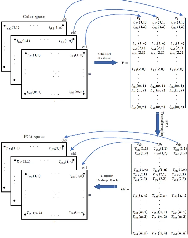
Original images in RGB space were transformed into HSI and LUV spaces as reported in (Sopharak, Uyyanonvara et al. 2008, Welfer, Scharcanski et al. 2010). Principal component analysis (PCA) was later applied on the images for the three color spaces. The rationale behind the transformation is based on the study by Unnikrishnan et al. (Unnikrishnan, Aliahmad et al. 2013) which showed that application of PCA on the RGB space can provide eigenchannels with better contrast between background and foreground objects compared to the green channel. In this study, we used PCA transformation on each color space (RGB, HSI and LUV) and the procedure is described below.

PCA on an Image

By applying PCA on an image with three channels, three eigenchannels (principle components) are created. It is assumed that intensity of a pixel (P) for an image (I) is presented by the equation 2.1:

(47)

42

𝑃_(𝑥,𝑦) = (𝐼_𝑐ℎ1(𝑥, 𝑦), 𝐼𝑐ℎ2(𝑥, 𝑦), 𝐼𝑐ℎ3(𝑥, 𝑦)); 1 ≤ 𝑥 ≤ 𝑚, 1 ≤ 𝑦 ≤ 𝑛 (3.15)

where IchZ corresponded to intensity of Zth (1 ≤ Z ≤ 3) channel (Ich) and (x, y) is the location

of the pixel. To apply PCA on an image, each channel is reshaped to a vector (vz) with size

of [1, m × n] and, consequently, that creates matrix V = [v1 v2 v3] where vz is described in

3.16: 𝑉 = [ 𝑣₁ 𝑣₂ 𝑣₃ 𝐼𝑐ℎ1(1,1) 𝐼𝑐ℎ2(1,1) 𝐼𝑐ℎ3(1,1) 𝐼𝑐ℎ1(1,2) 𝐼𝑐ℎ2(1,2) 𝐼𝑐ℎ3(1,2) ⋮ ⋮ ⋮ 𝐼_𝑐ℎ1(1, 𝑛) 𝐼_𝑐ℎ2(1, 𝑛) 𝐼_𝑐ℎ3(1, 𝑛) 𝐼𝑐ℎ1(2,1) 𝐼𝑐ℎ2(2,1) 𝐼𝑐ℎ3(2,1) 𝐼𝑐ℎ1(2,2) 𝐼𝑐ℎ2(2,2) 𝐼𝑐ℎ3(2,2) ⋮ ⋮ ⋮ 𝐼_𝑐ℎ1(2, 𝑛) 𝐼_𝑐ℎ2(2, 𝑛) 𝐼_𝑐ℎ3(2, 𝑛) ⋮ ⋮ ⋮ 𝐼𝑐ℎ1(𝑚, 1) 𝐼𝑐ℎ2(𝑚, 1) 𝐼𝑐ℎ3(𝑚, 1) 𝐼_𝑐ℎ1(𝑚, 2) 𝐼_𝑐ℎ2(𝑚, 2) 𝐼_𝑐ℎ3(𝑚, 2) ⋮ ⋮ ⋮ 𝐼_𝑐ℎ1(𝑚, 𝑛) 𝐼_𝑐ℎ2(𝑚, 𝑛) 𝐼_𝑐ℎ3(𝑚, 𝑛)] (3.16)

In the next step, PCA was applied on V to produce eigenvector matrix EG = [eg1 eg2 eg3],

where egz corresponds to Zth eigenvector and TchZ (m,n) stands for value of PCA

(48)

43 𝐸𝐺 = [ 𝑒𝑔1 𝑒𝑔2 𝑒𝑔3 𝑇𝑐ℎ1(1,1) 𝑇𝑐ℎ2(1,1) 𝑇𝑐ℎ3(1,1) 𝑇_𝑐ℎ1(1,2) 𝑇_𝑐ℎ2(1,2) 𝑇_𝑐ℎ3(1,2) ⋮ ⋮ ⋮ 𝑇𝑐ℎ1(1, 𝑛) 𝑇𝑐ℎ2(1, 𝑛) 𝑇𝑐ℎ3(1, 𝑛) 𝑇𝑐ℎ1(2,1) 𝑇𝑐ℎ2(2,1) 𝑇𝑐ℎ3(2,1) 𝑇_𝑐ℎ1(2,2) 𝑇_𝑐ℎ2(2,2) 𝑇_𝑐ℎ3(2,2) ⋮ ⋮ ⋮ 𝑇_𝑐ℎ1(2, 𝑛) 𝑇_𝑐ℎ2(2, 𝑛) 𝑇_𝑐ℎ3(2, 𝑛) ⋮ ⋮ ⋮ 𝑇_𝑐ℎ1(𝑚, 1) 𝑇_𝑐ℎ2(𝑚, 1) 𝑇_𝑐ℎ3(𝑚, 1) 𝑇_𝑐ℎ1(𝑚, 2) 𝑇_𝑐ℎ2(𝑚, 2) 𝑇_𝑐ℎ3(𝑚, 2) ⋮ ⋮ ⋮ 𝑇𝑐ℎ1(𝑚, 𝑛) 𝑇𝑐ℎ2(𝑚, 𝑛) 𝑇𝑐ℎ3(𝑚, 𝑛)] (3.17)

Each eigenvector was reshaped back to the original image size [m,n] to obtain an image in the space corresponding to PCA of original color space. Figure 2.13 shows the schematic of the transformation method. After applying this to the three color spaces (RGB, HSI and LUV), it resulted in three new spaces. The total of six color spaces (three original and three PCA) were used for further analysis.

(49)

44

(50)

45

Introducing New Color Space

The different color spaces were ranked based on the CNN performance measured using accuracy of classification. The new color space was identified experimentally by combining sets of three high ranking channels and comparing their performances. To reduce the number of combinations, a selection rule was formulated to combine only those channels with the low similarities measured using structural similarity index method (SSIM) (Wang, Bovik et al. 2004) (equation 3.18). This was calculated between each channel of the image against rest of the channels and ranked based on their similarity with the target channel.

𝑆𝑆𝐼𝑀(𝑥, 𝑦) = (2𝛼𝑥𝛼𝑦+ 𝑐1)(2𝜎𝑥𝑦+ 𝑐2) (𝛼𝑥2+ 𝛼𝑦2+ 𝑐1)(𝜎𝑥2+ 𝜎𝑦2+ 𝑐2)

(3.18) where 𝛼_𝑥, 𝛼_𝑦, 𝜎_𝑥, 𝜎_𝑦and 𝜎_𝑥𝑦are the local means, standard deviations and cross-covariance for images x and y, respectively. 𝑐₁ = (0.01 × 𝐿)2 and 𝑐₁ = (0.03 × 𝐿)2, where L is dynamic range of the pixel-values. The SSIM is a value between -1 and +1, +1 indicates that the two images are identical. By comparing all the possible pairs from the nominated channels, the channels were ranked and the three channels with lowest similarity index were identified to form the new space. In the next step, the CNN was trained and tested to distinguish between exudates and non- exudates patches.

3.3.2

CNN-Based Method

To assess the performance of different color spaces for exudate detection, a CNN model was developed, and its architecture is described in Table 2.2.

(51)

46

Table 2.2. Architecture of the proposed CNN. I - Input image, C - Convolutional layer, MP - Max pooling layer, FC - fully-connected, FM - Feature map, CH - Channels, Neurons-N.

Layer Type Feature Maps and Neurons Filter Size Weights

0 I 3CH-25×25 - - 1 C 16FM-23×23N 3×3 448 2 MP 16FM-12×12N 2×2 - 3 C 16FM-10×10N 3×3 2,320 4 C 16FM-8×8N 3×3 2,320 5 MP 16FM-4×4N 2×2 - 6 C 16FM-2×2N 3×3 2,320 7 MP 16FM-1×1N 2×2 - 8 FC 100N 1× 1 202

In this architecture, four convolutional layers were used with 16 feature maps in each layer of size 3 × 3 pixels. Rectified linear unit (ReLU) was used as the neuron activation function to ensure that the output was positive. Max-pooling layers of the size 2 × 2 pixels were used after the first, third and fourth convolutional layer. For updating network parameters, backpropagation training approach and stochastic gradient descent (SGD) was used.

3.4

Material

Two publicly available databases were used in this chapter and are described below:

DIARETDB1

The DIARETDB1 database (Kauppi, Kalesnykiene et al. 2007) consists of 89 color retinal images of the size 1500 × 1152. All images were taken by digital fundus camera with a 50

(52)

47

degree field of view and there are differences between the quality of the different images. The exudates have been manually annotated and evaluated by four independent medical experts. In this work, hard and soft exudates were grouped together and considered as a single class. The Figure 2.14 on the left shows an example of a manually segmented retinal image of a diabetic patient with exudates marked in blue while on the right shows the retinal image of a healthy subject with no sign of exudate. It can be seen that the size of the exudate’s sp