Visual Saliency Estimation Via HEVC
Bitstream Analysis
Submitted by:
XU DAI
For the degree of
Master of Philosophy
The University of Sheffield
Department of Electronic and Electrical Engineering
September 8
th, 2017
1
Abstract
Since Information Technology developed dramatically from the last century 50's, digital images and video are ubiquitous. In the last decade, image and video processing have become more and more popular in biomedical, industrial, art and other fields. People made progress in the visual information such as images or video display, storage and transmission. The attendant problem is that video processing tasks in time domain become particularly arduous.
Based on the study of the existing compressed domain video saliency detection model, a new saliency estimation model for video based on High Efficiency Video Coding (HEVC) is presented. First, the relative features are extracted from HEVC encoded bitstream. The naive Bayesian model is used to train and test features based on original YUV videos and ground truth. The intra frame saliency map can be achieved after training and testing intra features. And inter frame saliency can be achieved by intra saliency with moving motion vectors. The ROC of our proposed intra mode is 0.9561. Other classification methods such as support vector machine (SVM), k nearest neighbors (KNN) and the decision tree are presented to compare the experimental outcomes. The variety of compression ratio has been analysis to affect the saliency.
2
Acknowledgements
First and foremost, I would like to show my deepest gratitude to my supervisor Dr. Charith Abhayaratne, a respected scholar who has provided me with valuable guidance in my research period. Without his enlightening instruction, impressive kindness and patience, I could not have completed my study.
Also, I would like to thank everyone in our research group and my friend Zheng Hui for their support. Finally, I would like to thank my parents and my every family members. They give me very big support.
3
Contents
Chapter 1. Introduction ... 10
1.1. Motivations... 10
1.2. Aims and Objectives... 11
1.3. Contribution ... 12
1.4. Thesis Outline ... 12
Chapter 2. Literature Survey ... 14
2.1. Visual attention mechanism ... 14
2.1.1. Human Visual System... 14
2.1.2. Visual attention mechanism model ... 15
2.2. Psychology and neurobiology of visual attention ... 17
2.2.1. Bottom-up and top-down selective attention ... 17
2.2.2. Explicit attention and implicit attention ... 17
2.3. Visual searching ... 18
2.3.1. Inhibition mechanism in visual attention ... 18
2.3.2. Resolution and multi-scale of selective visual attention ... 19
2.4. Visual attention mechanism model ... 19
2.4.1. Filter model ... 19
2.4.2. Response selection model ... 20
2.4.3. Resource allocation model ... 20
2.4.4. Binary theory ... 20
2.5. Basic features of image and video ... 21
2.5.1. Brightness ... 21
2.5.2. Color ... 21
2.5.3. Three primary colors ... 22
2.5.4. RGB color space ... 22
4
2.5.6. Texture ... 23
2.5.7. Motion... 24
2.6. Saliency model ... 24
2.6.1. Static image saliency ... 25
2.6.2. Video saliency estimation ... 31
2.6.3. Applications of saliency model ... 34
2.7. High Efficiency Video Coding (HEVC) ... 35
2.7.1. Video coding system ... 35
2.7.2. HEVC Introduction ... 35
2.7.3. HEVC Coding structure ... 37
2.7.4. Prediction blocks ... 39
2.7.5. Intra prediction ... 41
2.7.6. Inter prediction ... 43
2.7.7. Transform and quantization ... 44
2.7.8. In-loop filtering ... 47
2.7.9. Decoded picture buffer ... 48
Chapter 3. Visual saliency estimation via HEVC bitstream analysis ... 49
3.1. Introduction ... 49
3.2. Experimental Datasets ... 49
3.3. Developer tools ... 51
3.4. HEVC encoding profile and configuration ... 51
3.4.1. Intra ... 52
3.4.2. Low delay ... 53
3.4.3. Random access ... 54
3.5. HEVC Feature analysis ... 54
3.5.1. Low-level features ... 55
3.5.2. High-level features ... 65
3.6. Proposed method ... 67
3.6.1. Beysian theory ... 68
3.6.2. Naïve Bayesian classification... 68
3.6.4. K nearest neighbors algorithm ... 71
5
3.6.6. Intra-frame prediction model ... 72
3.6.7. Inter-frame saliency prediction model ... 74
3.7. Experimental Result Analysis ... 75
3.7.1. Intra frame model ... 75
3.7.2. Inter frame model ... 80
3.8. Compression ratio ... 82
Chapter 4. Conclusion and further work ... 85
4.1. Conclusion ... 85
6
List of Figures
Figure 1-1 The applications of compressed video. ... 11
Figure 2-1: Information perception processing of Human visual perception system. .... 14
Figure 2-2Human eye structure schematic diagram [57]. ... 15
Figure 2-3 Illustration of Visual Attention. a) Intensity contrast b) Colour contrast c) Orientation contrast. ... 16
Figure 2-4 Illustration of Filter Model. ... 20
Figure 2-5 Illustration of Koch & Ullman selective processing model. ... 26
Figure 2-6 llustration of Itti selective visual attention model. ... 27
Figure 2-7 Illustration of Cheng motion saliency visual attention model. ... 32
Figure 2-8 Video coding system. ... 35
Figure 2-9 HEVC video decoder processing. ... 37
Figure 2-10 Closed GOP structure. ... 38
Figure 2-11 Opened GOP structure. ... 38
Figure 2-12 CU quad-tree syntax. ... 40
Figure 2-13 The block partitions in HEVC. ... 41
Figure 2-14 Intra prediction modes and directions of angular prediction. [58] ... 42
Figure 2-15 Four patterns of adjacent samples in SAO. C is the center sample and a and b is two adjacent samples. (a) horizontal location, (b) vertical location, (c) 135⁰ diagonal location, (d) 45⁰ diagonal location. ... 48
Figure 3-1 The thumbnails of test sequences in dataset. ... 50
Figure 3-2 Intel Video Pro Analyzer 2016 evaluation mode. ... 51
Figure 3-3 All intra-decoded sequence. ... 53
Figure 3-4 Low delay decoded sequence. ... 53
Figure 3-5 Random access decoded sequence. ... 54
Figure 3-6 Block depth feature map in intra main configuration. First row: original frames in intra mode. Second row: block depth map in intra mode. ... 56
Figure 3-7 Number of saliency/non-saliency pixels in different block depth in intra main configuration. Left: Before unify. Right: After unify. ... 56
7
Figure 3-8 Block depth feature map in low delay configuration. First row: original frames in low delay mode. Second row: block depth map in low delay mode. ... 57 Figure 3-9 Number of saliency/non-saliency pixels in different block depth ... 57 Figure 3-10 Example of all skip inter frame. ... 58 Figure 3-11 Block depth feature map in random access configuration. First row: original frames in random access mode. Second row: block depth map in random access mode. ... 58 Figure 3-12 Number of saliency/non-saliency pixels in different block depth ... 59 Figure 3-13 ADI feature analysis. Top left: an Original frame with ADI information. Top right: ADI feature map. Bottom: ADI value distribution in saliency and non-saliency pixels. ... 61 Figure 3-14 ADI and Saliency distribution in different videos... 62 Figure 3-15 Motion vector movement comparison. Left: Image of saliency object with small amount of movement. Right: Image of saliency object with large amount of movement. ... 64 Figure 3-16 Inter frame motion vector in video encoded with different configurations.
... 64 Figure 3-17 Residual of a frame in different video configuration. Left to right: Original frame; All intra configuration; Low delay configuration; Random access configuration. ... 66 Figure 3-18 : Prediction of a frame in different video configuration. Left to right: Original frame; All intra configuration; Low delay configuration; Random access configuration. ... 66 Figure 3-19 : Comparison between original reconstructed prediction data and simplified reconstructed prediction data. Left: original reconstructed prediction frame. Right: simplified reconstructed prediction frame. ... 74 Figure 3-20 Intra-frame saliency results of static background set. First column : Original frame. Second column: GBVS image saliency. Third column: Itti’s image saliency. Fourth column: Proposed method (Bayesian model). Fifth column: Manual
8
segmented ground truth. ... 76 Figure 3-21 Intra-frame saliency results of dynamic background set. First column : Original frame. Second column: GBVS image saliency. Third column: Itti’s image saliency. Fourth column: Proposed method (Bayesian model). Fifth column: Manual segmented ground truth. ... 77 Figure 3-22Intra-frame saliency results of objects moving with dynamic background set. First column : Original frame. Second column: GBVS image saliency. Third column: Itti’s image saliency. Fourth column: Proposed method (Bayesian model). Fifth column: Manual segmented ground truth. ... 77 Figure 3-23 Intra-frame saliency results of moving camera. First column: Original frame. Second column: GBVS image saliency. Third column: Itti’s image saliency. Fourth column: Proposed method (Bayesian model). Fifth column: Manual segmented ground truth. ... 78 Figure 3-24 Intra frame ROC comparison between existing model and proposed model. ... 80 Figure 3-25 Inter-frame saliency results. First column: Original frame. Second column: Itti motion saliency. Third column: Proposed method with low delay configuration. Fourth column: Proposed method with random access configuration. Fifth column: Manually segmented ground truth from dataset. ... 81 Figure 3-26 ROC curve of one video sequence. ... 82 Figure 3-27 Intra-frame saliency results. First column: Original frame. Second column: Proposed method (Bayesian model). Third column: Manual segmented ground truth. First row: qp=16. Second row: qp=32. Third row: qp=51. ... 82 Figure 3-28 Inter-frame saliency results. First column: Original frame. Second column: Proposed method (Bayesian model). Third column: Manual segmented ground truth. First row: qp=16. Second row: qp=32. Third row: qp=51. ... 83 Figure 3-29 ROC curve of different QP values. ... 83
9
List of Tables
Table 2-1 The comparison of video saliency estimation in compressed domain... 34 Table 3-1 HEVC configuration. ... 52 Table 3-2 Intra frame performance comparison between existing model and proposed model. ... 79
10
Chapter 1. Introduction
With the rapid development of information technology, image video information is growing and expanding. Computers are a useful tool in information analysis and large amounts of data processing. However, the speed of multimedia data growth is much greater than the speed of computer processing performance [1]. In addition, People only concern a part of a given image (or a video). This is because the amount of data in the image/video is beyond the processing power of the human eye [2]. Therefore, the ability to predict where humans' attention becomes a popular research content.
In recent years, network bandwidth and storage have increased rapidly, but it is far from meeting the requirements for the transmission and storage of massive video data. Therefore, the efficient compression of video information is one of the important technical measures to solve this contradiction. Video compression technology has been concentrated in the past two to three decades. From the first video coding standard H. 261 / MPEG-1 [3], the second generation of video coding standard H. 264 / AVC [3], and the third generation of video coding standard High Efficiency Video Coding (HEVC), the efficiency of video compression for each generation greatly increased. This thesis focus on the saliency estimation in HEVC compression domain.
1.1.
Motivations
With the rapid development of science and information technology, video resolution is from early 176 x 144, 352 x 288, 416 x 244, 720 x 480, 1280 x 720, and 1920 x 1080. Now ultra-high-definition (3840x2160) videos also cut a striking figure. With the increasing amount of video data, the existing video processing technology is not mature enough to deal with such a huge amount of data, real-time video processing tasks become particularly arduous.
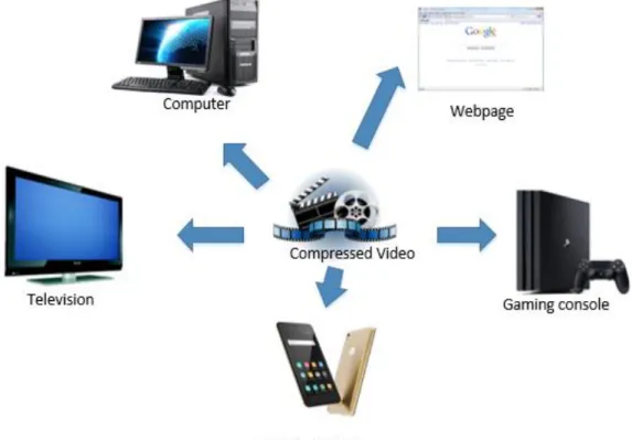
Currently, video saliency detection has been widely applied to many video processing applications such as video compression based on video highlighting, video classification, video watermarking, video transcoding, and video scaling. Visual
11
attention analysis simulates the human eye vision system by automatically detecting the salient region of the acquired image. In image processing, the research of video saliency is practically important.
Figure 1-1 The applications of compressed video.
1.2.
Aims and Objectives
The main aim of this thesis is to estimate video saliency using Bayesian modeling of HEVC features in the compressed domain.
Our model is used in video saliency estimation. This can be summarized by the following objectives:
To research the state-of-the-art of saliency estimation methods in both image and video domain. The gaps of the existing methods are analyzed.
To study the High Efficiency Video Coding (HEVC). The decoder part of HEVC is introduced. The good standing of HEVC decoder can help us to find the relationship between HEVC bitstream features and saliency.
12
within features extracted from HEVC compressed domain. All extracted features are analyzed and evaluated in different HEVC compressed mode. A naïve Bayesian classifier is trained for saliency region estimation in videos.
Different machine learning classification algorithms such as support vector machine (SVM), k nearest neighbors (KNN) and the decision tree are presented to compare the experimental outcomes. The variety of compression ratio has been analysis to affect the saliency.
1.3.
Contribution
A new proposed video saliency model in the compressed domain is proposed in this thesis. The relative intra and inter features such as block size, residuals, intra mode difference, motion vectors are extracted from HEVC decoder. Both intra mode saliency and inter saliency are achieved. The novelty of this model is to achieve saliency map in HEVC compressed domain without fully decoded bitstream. This method can be used in image/video searching and visual interface design.
Bayesian model is used for training and classification for the salient regions for each frame. The testing videos are divided into two parts: half of testing videos are used to training and half of them are used to classification. The basic theory of Bayesian model is classifying features to maximum probability category. The variety of compression ratio has been analysis to affect the saliency.
1.4.
Thesis Outline
The reminder of the thesis is structured as the following chapters. The contents of each chapter are summarized.
In chapter 2, the state-of-the-art for visual saliency is reviewed and presented. The chapter includes background of visual attention and visual attention models (VAM) in single image or a video. The comparison of video saliency estimation in the compressed domain is also provided. The applications of visual attention model are presented. General features used in the saliency estimation are introduced in detail. Then an
13
overview of HEVC coding system is provided. Some important HEVC decoder block coding steps is introduced briefly.
Chapter 3 analyzes and evaluates all extracted features are in different HEVC compressed mode. Then, a new video saliency method in video compressed domain is proposed.The intra saliency estimation is achieved using naïve Bayesian classification by relative HEVC features. The inter saliency is achieved by intra saliency moving via motion vector. Different machine learning classification algorithms such as support vector machine (SVM), k nearest neighbors (KNN) and the decision tree are presented to compare the experimental outcomes. The variety of compression ratio has been analysis to affect the saliency. The results are evaluated by ROC curve.
Chapter 4 includes a brief summary of the whole thesis. Some suggested further work is provided.
14
Chapter 2. Literature Survey
This chapter contains background of human visual system and visual attention models. Some existing image and video saliency models are presented. The applications of visual attention in different areas are discussed. The image/video features are introduced.
2.1.
Visual attention mechanism
With the rapid development of information technology, images and videos have become an important carrier of information. Processing and analysis digital image and video data efficintly has become the central issue.
2.1.1. Human Visual System
On the human visual perception system and visual nervous system, psychology and other related fields experts have carried out long-term exploration [4] and research. Through deeply research and exploration, visual sensory information in the visual nervous system is in accordance with a fixed path to be transmitted. The input is visual stimulation, the output is visual perception. The human visual system is mainly composed of visual sensory [5], visual pathway, visual central nervous system [6] and visual perception central organization.
15
The average diameter of person's eyes is about 24 mm [7]. The human eye is approximately spherical and consists of two parts: the eye wall and the eyeball. Cornea and sclera are located in the outer layer of the eye wall, in which the cornea with refractive effect [54], can be reflected the light to the eyes, scleral protects the eyeball. The middle layer of the eye wall consists of iris and choroid, and the inner retina is composed of cone cells and rod cells. Visual information is transmitted as follows: visual stimulation from the light sensory cells, effect on the retina [8], and then through the optic nerve, optic tract and subcortical center, finally reach the visual cortex, causing visual perception. The so-called visual sensation refers to the light brightness; visual perception refers to the color, shape and other characteristics.
Figure 2-2Human eye structure schematic diagram [57].
The cornea of the eye is a transparent, highly curved refraction window. The cornea of the eye is a transparent, highly curved refraction window, and then partially blocked by the opaque iris surface. The pupil changes with the intensity of the light. Under normal lighting conditions, pupil is in a 4contraction state, to avoid the blurring caused by spherical aberration.
2.1.2. Visual attention mechanism model
Visual attention is essentially a biological mechanism which can select from the complex environment, and gradually remove the relatively unimportant information [9]. In this way, the complex external scene can be simplified and decomposed. The advantage of this mechanism is that: it allows us to focus the important information and
16
objects rapidly in an environment [53].
Figure 2-3 Illustration of Visual Attention. a) Intensity contrast b) Colour contrast c) Orientation contrast.
Researchers do a lot of exploration about the applications of visual attention in physiological sciences, psychological science, neuroscience and information science field. The essence and characteristics of visual attention include six aspects [10]:
Selectiveness: Selecting part of information.
Concentration: Excluding unrelated stimuli.
Search: Looking for part of the targets.
Activation: To cope with all possible stimuli.
Set: To accept and respond to specific stimuli.
Vigilance: Keeping long attention.
Perry and Hodges study the mechanism of visual attention in the perspective of neuroscience. The manifestations of visual attention are [15]:
Selective Attention and Shifting: The characteristic is to focus on dealing with a relevant stimulus at the same time while ignoring or discarding other irrelevant stimuli.
Sustained Attention: It is characterized by a long period to maintain concentration attention.
Divided Attention: It is characterized by distributing attention at the same time, focuses on dealing with multiply related stimuli.
Harris argues that "concentration" and "vigilance" are the most basic features of the attention mechanism and, based on which visual attention is divided into four types:
17
Selective Attention: Used to select part of the visual information to meet the brain's limited information processing needs.
Parsing Attention: Used to separate the target from the background for pattern recognition.
Directing Attention: Used to guide the emergency interruption, the normal detection, and maintenance of visual attention and other acts of switching;
Alertness Attention: Used to wake up the potential visual information processing.
2.2.
Psychology and neurobiology of visual attention
The main research of visual selective attention mechanism on psychology and neurobiology in the following aspects.
2.2.1.
Bottom-up and top-down selective attention
The visual selective attention mechanism can be generalized in two aspects: bottom-up selective attention [11] and top-down selective attention [11]. Bottom-up [12] selective attention is driven by pure external stimuli, such as a strong contrast. The top-down selective attention is controlled by the subject, which is controlled by high-level brain information such as knowledge, expectations, and goals [12]. In the same scene, different people get the results of attention are different. Current research on top-down factors is limited and often manifested in obtaining knowledge related to target objects. Other top-down factors such as motivation, expectation, emotion, etc. are more difficult to control and analyze.
2.2.2.
Explicit attention and implicit attention
In general, explicit attention refers to the transfer of the region of interest, which is associated with the movement of the eye. Because the center of the human eye has a high resolution but a low resolution in the surroundings, the explicit attention happens when the area of selective visual attention falls away from the place where the current
18
fixation point is distant or even outside the field of view [13, 52]. In addition, there is another situation, which is not accompanied by the transfer of gaze. In 1890, William James pointed out that we can move attention without eye movement [52]. This phenomenon is implicit attention. For example, when you walk down the street to see the front, you will not bump the pedestrian next to you. Implicit attention is more efficient than explicit attention.
2.3.
Visual searching
Visual searching is an important tool in the study of visual attention. In the visual psychology experiment, the subjects are required to find certain requirements of the target around many interference objects [14]. One of the parameters of the visual searching efficiency is the reaction time. The research demonstrated that the response time almost unchanged as the number of interfering objects increases sometimes. However, in some cases, the reaction time increases rapidly as the number of interfering objects increases.
There are many theories to explain the essential difference between the selective attention mechanism in the efficient and inefficient search. The influential theory is Treisman's characteristic fusion theory. Feature fusion theory states that when the target can be distinguished by a feature, and the other disturbances have the same characteristics, the target is detected easily, quickly and in parallel. That theory holds that each object is processed in parallel in an efficient visual searching, while the object is processed serially during an inefficient searching. When the difference between the target object and the interfering objects is a combination of multiple features, the search belongs to serial searching.
2.3.1.
Inhibition mechanism in visual attention
The inhibition of selective attention is widely studied. One of the most common studied phenomena is the inhibition of return. It means that the respondent has slowed down the target response that had previously been repeated in the same position. It has been
19
argued that the inhibition of return mechanism plays an important role in maintaining spatial selectivity [15]. It enables the tester to return to the location where the target information has been extracted. Inhibition of return has important implications, for example, people do not repeatedly detect the same interfering object in visual search. inhibition of return [22].
2.3.2.
Resolution and multi-scale of selective visual attention
The resolution of selective visual attention refers to the ability to distinguish a single object in a number of closely arranged objects. It is common to use a plurality of interfering objects around the target to investigate how far the interfering object will affect the test object [16, 56]. It is used to study the resolution of the selective attention. When the distance between two objects is less than the resolution, people will not notice the single object. This phenomenon is called the Crowding Effect [51]. Another problem with this is the multi-scale problem. Human visual perception is carried out at multiple scales. For example, when you want to get a book, you will first notice the bookcase and then find your book. The scale of searching is different.
2.4.
Visual attention mechanism model
Visual saliency have become a prerequisite for many computer vision algorithms. This includes selecting a block in the scene or selecting a combination of some features in the area. Selective visual attention mechanism is an effective way to improve the real-time complexity and to solve the problem of information explosion [17].
2.4.1.
Filter model
Broadbent proposed a filter model in 2001 [18]. The number of visual information input channels is greater than before. However, only one channel is accessed through the filter into the advanced analysis phase. This filter reflects the selection of visual attention. Once the information exceeds human’s acceptable capacity, the filter will lock the
20
redundant information. Only that information through the filter can be analyzed.
Figure 2-4 Illustration of Filter Model.
2.4.2.
Response selection model
Deutsch proposed response selection model [19]. All the visual information of multiple input channels can enter the advanced analysis phase. The perceptual processing is obtained. Visual attention is not the choice of visual stimulus, but rather the choice of response to stimulation.
2.4.3.
Resource allocation model
Kahneman proposed the resource allocation model [20]. It thought visual attention is essentially a resource allocation mechanism. It allocates human limited information processing capacity (resources) according to a resource allocation scheme under various constraints. The selectivity of visual attention is manifested through this resource allocation scheme.
2.4.4.
Binary theory
The binary theory was proposed in the 1990s [21]. Visual information processing methods are divided into control processing and automatic processing. The characteristics of control processing are:
21
Under the conscious control.
Limited capacity.
Slow and flexible.
The characteristics of automatic processing are:
It does not need to pay attention to participation.
Free from conscious control.
Great capacity.
Faster but lack of flexibility.
2.5.
Basic features of image and video
2.5.1.
Brightness
The luminous intensity of the visual scene is called brightness. The human eye has a strong sensitivity to the brightness, which determines the brightness is an important factor of saliency detection. In the field of digital image processing, grayscale [23] can be used to represent the brightness. The brightness level of the image is presented using black with different saturation. The brightest represent by white and the darkest represent by black. Each grayscale object has a luminance value in the range 0% -100%. 0% represent white and 100% represent black. For 8-bit images, the luminance values are quantized and the range can be normalized to [0,255] intervals. The 256 discrete gray scale represents the different brightness of the image.
2.5.2.
Color
For different wavelengths of visible light, the human visual system has different subjective feelings. The different performance lies in different colors. Color is one of the most important elements of the image. The human visual system is more sensitive to color. In the image processing, the color characteristics can be described by the existing color space. Different color spaces are available for different applications. Color TV uses YUV as the color space, in order to use the brightness signal Y to solve
22
the compatibility issues. So that black and white TV can also receive color TV signals.
2.5.3.
Three primary colors
The human eye has a different sensitivity for different colors because the human eye has several kinds of conical photoreceptor cells. These cells are most sensitive to green, yellow-green and violet light. Their wavelengths are 534nm, 564nm, and 420 nm respectively [24]. If the stimuli of yellow-green photoreceptor cells is greater than the stimuli of green photoreceptor cells, people will recognize yellow; if the stimuli of yellow-green photoreceptor cells is much higher than the stimuli of green photoreceptor cells, people will recognize red. Although the three photoreceptors are not the most sensitive to green, red and blue. These three colors can stimulate the photoreceptors. Therefore, the green, red and blue as the basis of color perception. These three colors called primary colors.
2.5.4.
RGB color space
Based on the principles of the human visual system described above, red, green, and blue colors are set as the reference colors of RGB color space [25]. Variety of different colors are formed by different weights between three colors. RGB color space almost includes all perceived colors.
2.5.5.
YUV color space
In YUV color space, "Y" is the luminance, that is, the gray scale value. "U" and "V" are the color components. The specific part of the RGB signal is superimposed to establish the luminance signal. The RGB color space and the YUV color space conversion are shown below [26]:
[ 𝑅 𝐺 𝐵 ] = [ 1 −0.00093 1.401687 1 −0.3437 −0.71417 1 1.77216 0.00099 ] [ 𝑌 𝑈 − 128 𝑉 − 128 ]. (2-1)
23 [ 𝑌 𝑈 𝑉 ] = [ 0.299 0.587 0.114 −0.169 −0.331 0.5 0.5 −0.419 −0.081 ] [ 𝑅 𝐺 𝐵 ] + [ 0 128 128 ]. (2-2)
2.5.6.
Texture
Compared with intensity and color features, texture belongs to the advanced saliency characteristics. The external manifestation of the surface change or distribution of the object is called texture. The texture is often expressed as color or light of a regular change [27]. It can be seen that the human vision system can quickly determine the surface with different textures. However, it is difficult to know how the human visual system is handled. In addition, it is difficult to use language or text to describe in detail [28]. One of the most popular view states that the texture primitives form a texture according to a regular distribution such as zebra or tiger body stripes. Usually, this law has a certain uniformity, repeatability, and directionality [62, 63]. The above properties are also the basis of texture analysis.
Texture analysis methods are generally region-based because texture has a strong regional nature. Texture analysis refers to the use of a certain image processing technology is to extract the texture parameters, which can be a quantitative or qualitative description of the texture processing. Texture analysis can be divided into three types: structural methods, statistical methods, and spectrum methods. Structural methods refer to the analysis of the structure of the region to get the texture elements, and then use the texture elements to describe the texture of the image. Statistical methods refer to the analysis of the texture properties of the color distribution in the observation area. The main algorithm is random field model, random classification model and gray level co-occurrence matrix. Spectrum methods refer to the Garbo transform, Fourier transform or wavelet transform to obtain the coefficients to describe the texture. The Tamura parameter and the gray level co-occurrence matrix are more effective spectrum method.
24
2.5.7.
Motion
Motion as a description of the video content cannot be ignored in computer vision. Motion is also an indispensable feature for extracting video prominence regions [28]. People tend to concern objects with fast and strenuous moving. The features for the image mainly focus on color, brightness, texture; the main features of the video focus on the motion.
For non-compressed domain videos, the main methods of motion detection are optical flow [62] and frame difference [63]. The optical flow method can be considered as the motion of the image luminance mode in the video sequence, also it can be considered as the representation of the velocity of the motion on the surface of the object. The frame difference method is the subtraction between the adjacent frames; the difference is taken as the motion information.
For the compressed domain videos, inter frame predictive coding is used to remove temporal redundancy between adjacent frames. Inter frame prediction coding mainly uses the time domain correlation between successive frames to eliminate the time redundancy by motion compensation. Each frame in the video is divided into blocks, and each block is encoded. The target frame encoder requires the use of blocks of previously encoded video frames. The relative position difference between the target code block and the reference code block is called motion vector. The motion vector is the motion information of the compressed domain video. Therefore, the motion vector in the bitstream can be extracted. In addition, using motion vector need to take into account the camera movement and other factors. In the event of camera shake, the background has motion relative to the foreground, thus affecting the motion vector accuracy.
2.6.
Saliency model
In visual attention models, saliency map is used to define the visual attention area. Saliency map is a two-dimensional map of the same size as the original image, where
25
each pixel value represents the visual attention of the corresponding image. Many methodologies in visual attention estimation of both Static or dynamic scene are presented in this section.
2.6.1.
Static image saliency
The first image saliency estimation algorithm is proposed by Koch and Ullman [11]. Although this model has not yet been implemented at the beginning of the presentation, it provides an algorithmic basis for future implementation. Many of current visual attention models are based on Koch and Ullman’s work. The main idea of this saliency estimation algorithm is to combine a number of features in parallel with a feedforward model. WTA (Winner-Take-All) competitive neural network is used to determine the most salient area. Then a suppression of return mechanism is used to move the gaze into next the most salient area. Koch and Ullman [5] proposed the WTA neural network (the neural network that determines the most salient area in topographic map) and the concrete description of the implementation. This WTA neural network approach has a strong biological motivation and shows how the human brain may achieve VA mechanism. However, for computer systems, the WTA is not necessary because there is a simpler way to determine the most salient area.
26
Figure 2-5 Illustration of Koch & Ullman selective processing model.
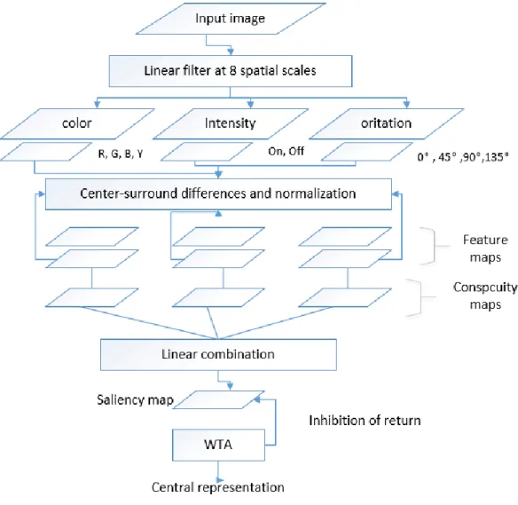
The first completed implementation of Koch and Ullman’s hypothesis is proposed by Koch & Ullman in 1994 [12]. Since then, visual attention estimation becomes more and more popular. The Neuromorphic Vision Toolkit (NVT) is one of the most well-known systems which is derived by Koch & Ullman. NVT has been developed over the years by Itti research groups. This model has developed under the efforts of the research team centered on Itti et al. Their models and implementation methods become the basis of many research groups. The feature maps, saliency maps, winner-take-all (WTA) neural network and Inhibition-of-return (IOR) are derived from Koch & Ullman model.
27
Figure 2-6 llustration of Itti selective visual attention model. This model can be described as followings:
1. Feature maps extraction. They represent the gray, color, and gradient directions of the original image at six different scales. Each feature is calculated by the center-surrounding differences operator.
2. Then superimposing these feature maps as three conspicuity maps by weight normalizing. Then adding three conspicuity maps as a saliency map via linear combinations.
3. The inhibition of return system suppresses the salient area in this saliency map so that the attention position autonomously points to the next position.
Every feature map is calculated using a center surrounding structure similar to the biological receptive field. Central surrounding structure means that typical visual
28
neurons are sensitive to small areas located in the center. In addition, stimuli in the wider, weaker regions around their central regions will suppress the response of the visual neurons. It is clear that such precise structures for local spatial discontinuities are particularly suitable for detecting areas that are prominent around their surroundings, which are also general principles of use in the retina, external geniculate and visual cortex.
Let 𝑟, 𝑔, 𝑏 correspond to the red, green and blue channels of the input image, the gray scale image 𝐼 is:
𝐼 =(𝑟+𝑔+𝑏)
3 . (2-3)
In order to separate the chrominance signal from the intensity, gray scale is used to normalize the 𝑟, 𝑔, 𝑏 channels, because the little brightness change in Chroma channel is difficult to recognize. So the normalization only applied in the position which the gray scale is greater than the maximum 1/10 on the original image, and other locations of the 𝑟, 𝑔, 𝑏 value is assigned to zero. According to the normalized 𝑟, 𝑔 and 𝑏, the established of four wide tuning of the color channel are:
Red: 𝑅 = 𝑟 −(𝑔+𝑏) 2 . (2-4) Green: 𝐺 = 𝑔 −(𝑟+𝑏) 2 . (2-5) Blue: 𝐵 = 𝑏 −(𝑟+𝑔) 2 . (2-6) Yellow: 𝑌 =(𝑟+𝑔) 2 − |𝑟−𝑔| 2−𝑏. (2-7)
Further, according to these color channels, four Gaussian pyramids 𝑅(𝜎), 𝐺(𝜎), 𝐵(𝜎), 𝑌(𝜎) can be established to multiple Gaussian blur, where 𝜎 ∈ (0, 1, … ,8) is the scale. The Gabor pyramids 𝑂(𝜎, 𝜃) used to represent the local orientation information, where 𝜎 ∈ (0, 1, … ,8) and 𝜃 ∈ (0, 450, 900, 1350) . Flicker pyramid 𝐹(𝜎) can be yielded.
Center surrounding operation is implemented as a difference between the fine and course of a given feature. Center-surrounding differences defined two scales: fine scale 𝑐 and coarser scale 𝑠 . Considering three kinds of features: grayscale, color and
29
orientation. If the central peripheral differential operation is ⊝, the gray scale feature can be obtained from the following equation:
𝐼(𝑐, 𝑠) = |𝐼(𝑐) ⊝ 𝐼(𝑠)|. (2-8) Which 𝑐 ∈ {2, 3, 4} and 𝑠 = 𝑐 + 𝛿, 𝛿 ∈ {3, 4}.
In a human visual system, this feature is detected by neurons that are sensitive to bright central dark surroundings or dark central bright surroundings.
The second feature is related to color. In the human visual cortex, there are four kinds of space and color double opponent: red/green, green/red, blue/yellow and yellow blue color pairs. In this model, the corresponding feature map to the red/green or green/red color pairs is:
𝑅𝐺(𝑐, 𝑠) = |𝑅(𝑐) − 𝐺(𝑐)) ⊝ (𝐺(𝑠) − 𝑅(𝑠))|. (2-9)
And the feature map corresponding to blue/yellow or yello/blue color pair is obtained from the following:
𝐵𝑌(𝑐, 𝑠) = |𝐵(𝑐) − 𝑌(𝑐)) ⊝ (𝑌(𝑠) − 𝐵(𝑠))|. (2-10)
Local orientation information is achieved by applying Gabor pyramids 𝑂(𝜎, 𝜃) . Orientation feature maps 𝑂(𝑐, 𝑠, 𝜃) is obtained by:
𝑂(𝑐, 𝑠, 𝜃) = |𝑂(𝑐, 𝜃) ⊝ 𝑂(𝑠, 𝜃)|. (2-11)
For each pixel of the input image, saliency map uses a scalar to characterize its saliency and to guide the selection of attention points based on the spatial distribution of the saliency. The difficulty of combining feature maps is that features are incomparable. Since all features are combined together, some salient targets that appear in some feature maps may be overwhelmed by a large number of noise or not salient objects. In the initial thesis of Itti et al., a normalization operator 𝑁(. ) is proposed to enhance the feature map with less salient peaks and to weaken the feature maps with large numbers of salient peaks. For each feature map, this operator includes:
1. Normalizing the feature values to a range of [0…𝑀] to eliminate the amplitude difference depending on the features.
2. Calculating the global maximum 𝑀 of the map and the average of the other local maximum 𝑚̅.
30
3. Multiplying the feature map by (𝑀 − 𝑚̅ )2.
Only considering the local maximum 𝑁(. ), the useful regions of the feature maps can be focus on while ignoring the uniform areas. The difference between the global maximum and all local maximum mean value reflects the difference between the most interested area and the average interested area. If the difference value is large, the region of most interested will be highlighted; if the difference value is small, it indicates that the feature maps do not contain any salient region. The biological basis of 𝑁(. ) is that: It approximates the cortical inhibition mechanism.
The feature maps are grouped into three conspicuity maps. As shown in the following: 𝐼̅ = 4 ⊕ 𝑐 = 2 𝑐 = 4 ⊕ 𝑠 = 𝑐 + 3 𝑁(𝐼(𝑐, 𝑠)). (2-12) 𝐶̅ = 4 ⊕ 𝑐 = 2 𝑐 = 4 ⊕ 𝑠 = 𝑐 + 3 [𝑁(𝑅𝐺(𝑐, 𝑠)) + 𝑁(𝐵𝑌(𝑐, 𝑠))]. (2-13) 𝑂̅ = ∑ 𝑁( 4 ⊕ 𝑐 = 2 𝑐 = 4 ⊕ 𝑠 = 𝑐 + 3 𝑁(𝑂(𝑐, 𝑠, 𝜃)) 𝜃∈{0,450,900,1350} ). (2-14)
𝐼̅ means intensity, 𝐶̅ means color and 𝑂̅ means orientation. And ⊕ means accumulation point by point.
The reason for the establishment of three normalized saliency feature description is: similarity features are highly competitive while different features will independently play a role in the feature map. These three feature descriptions are further normalized and summed to obtain a saliency 𝑆:
𝑆 = 1
3(𝑁(𝐼̅) + 𝑁(𝐶̅) + 𝑁(𝑂̅)). (2-15)
In the later work of Itti et al. [12], A number of feature combinations were compared, and it was found that normalizing each feature graph to a fixed dynamic range would show poor detection performance when detecting prominent targets in complex background. A possible way to improve performance is to obtain a linear combination of the feature maps. Although this method can highly improve the detection performance, it brings a difficulty of different models used in one application. Itti et al. [12] proposed a new feature combination strategy, on the basis of normalization, to
31
enhance the feature maps which have less salient peaks by the local nonlinear competition. This competition pattern is similar to the nonclassical inhibition observed by electrophysiology.
2.6.2.
Video saliency estimation
Researchers extend spatial attention studies to videos that contains a lot of motion. Cheng et al. [30] proposed a model of video saliency that combines motion. As shown in Figure 2-7, this video visual attention model analyzes the horizontal and vertical motion of the pixels in every frame. The input video is segmented into shots that contain motion gradient information. Each frame is then divided into frame segments that do not coincide with each other. For each frame segment, the motion information of the recorded camera is used to generate saliency after wards. At the same time, each feature model (such as brightness, color, motion, etc.) are calculated. Depending on the motion information of the camera, combinations of these feature maps. Finally, the overall saliency map was constructed. The area of visual attention in the video is represented by the saliency distribution.
32
Figure 2-7 Illustration of Cheng motion saliency visual attention model.
Bioman et al. [32] proposed a method of detecting irregularities in the temporal space domain of the video. The basis of this method is to compare 2-D and 3-D texture training data sets of the video blocks instead use the motion information, to obtain the information of the irregular motion information in the video. Meur et al. [33] proposed a time-space domain model based on visual attention, by analyzing affine parameters to generate saliency map.
Muthuswamy et al. [29] proposed a motion saliency detection model. The discrete cosine transform (DCT) coefficient and motion information are used to identify the motion saliency in MPEG-2. In MPEG-2, I frame refers to intra information compression; B and P frame refers to motion compensation compression with the reference I frame. The DCT coefficient of every macro block is obtained according to
33
the established partial decoder in the bitstream. Residual and motion vector are used to DCT coefficient de-quantization. The luma and chroma components of DCT coefficient are used to estimate spatial saliency. The motion saliency map is obtained by accumulating the motion vector map to improve the spatial saliency map.
Fang et al. [60] proposed video attention estimation model in MPEG-4. The features such as color information, luminance, and texture are extracted from DCT coefficients. The motion vectors are extracted from the bitstream. The intra prediction I frame saliency is estimated by color information, luminance, and texture which is relative with Itti’s image saliency model. The P and B frame saliency is estimated by applying Gaussian model to weight the static saliency and motion map.
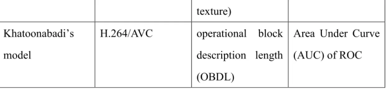
Khatoonabadi et al. [61] proposed a model to measure saliency using operational block description length (OBDL). This OBDL with minimum bits encoding in H.264/AVC compressed domain. When the prediction occur large errors, the residuals are large requiring more bits to code. OBDL can be calculated directly from decoder. According with OBDL, block size information from DCT coefficient can be extracted. Then Markov random field (MRF) is used to classify the block into saliency group or non-saliency group. The above methods can be summarized as following table.
Compressed method Features Performance evaluation Muthuswamy’s model MPEG-2 The DCT coefficient (luma and chroma components), motion vector Average Equalized Error Rate (EER) value
Fang’s model MPEG-4 The DCT
coefficient (color information, luminance and Receiver Operating Characteristic (ROC) curve
34
texture) Khatoonabadi’s
model
H.264/AVC operational block description length (OBDL)
Area Under Curve (AUC) of ROC
Table 2-1 The comparison of video saliency estimation in compressed domain.
As discussed with previous methods we can see that all techniques cannot cover the complex of HEVC features such as coding tree blocks splitting and bit locations. Moreover, none of the methods find the exact effect of features in the compressed domain to determinate the visual saliency. In fact, the relationship between the features in the compressed domain and the visual saliency can be achieved by training and testing the groundtruth and the video dataset. Therefore, this thesis presents a visual attention model of video by using HEVC features.
2.6.3.
Applications of saliency model
The visual attention model has been applied in many fields. Baccon et al. [34] proposed the use of visual attention techniques to select spatial-related visual information to control the direction of movement of the robot. Driscoll et al. [35] constructed a pyramid-type artificial neural network by calculating the two-dimensional saliency of the surrounding environment to control the focus of the camera. Chen et al. [36] applied visual attention techniques to small picture displays. The salienct regions have higher priority than other regions. Ouerhani et al. [37] and Stentiford [38] applied the attention model to image compression; the high saliency regions have higher compression quality.
35
2.7.
High Efficiency Video Coding (HEVC)
2.7.1.
Video coding system
Figure 2-8 Video coding system.
Figure 2-8 provides an overview of HEVC video coding system. These functions of blocks are indicated as below:
Video source: A video sequence is in a digital format acquired.
Pre-Processing: Some pre-operations such as trimming [31], color correction or de-noising.
Encoding: Operation of transform input sequence as a bitstream which can fit for the transmission scenario.
Transmission: Transmit the coded bitstream to the receiver.
Decoding: Processing bitstream into the reconstruction video. The reconstructed video is not the input sequence, as the encoding will occur compression loss.
Display: The final video to view. Some color format of the video needs to change in this processing.
2.7.2.
HEVC Introduction
The HEVC video coding compression standard is mainly developed by two major international organizations: ITU-T (International Telecommunication Union
36
Telecommunication Standardization Department) and ISO / IEC (International Organization for Standardization / International Electrotechnical Commission). ITU-T developed H.261 [32] and H.263 [32]; ISO / IEC developed MPEG-1 and MPEG4 [33]. These two organizations have developed H.262 / MPEG-2 video and H.264 / MPEG-4 AVC together. The co-developed video standards have been widely used, especially H.264 / MPEG-4 AVC [68]. Its applications include high-definition satellite television broadcasting, cable television, video capture / editing system, portable cameras, video surveillance, network and mobile Internet video transmission, Blu-ray discs, and real-time video applications such as video chat, video conferencing and telepresence systems. H.264 / MPEG-4 AVC basically covers all digital video applications and replaces other video compression standard.
However, with the increase in service diversification, the development of high-definition video and the emergence of ultra-high-high-definition format (4k × 2k or 8k × 4k), the market requires better video compression coding standards than H.264 / MPEG-4 AVC. In addition, with the rise of mobile devices and tablet PCs, demand for video services is increasing. Video quality and resolution requirements are increasing as well. These cause challenges to existing network bandwidth. Therefore, HEVC (High Efficiency Video Coding) as a new generation of video coding standards came into being. HEVC is composed of ITU-T VCEG (Video Coding Expert Group) [37] and ISO / IEC MPEG (Moving Picture Experts Group) [37]. JCT-VC began its first meeting in April 2010, to collect new video coding standard proposals from major companies, universities and research institutions in the world. The first version of HEVC was released in January 2013. The basic framework and content of HEVC were determined. HEVC continued to expand its content and functionality to adapt different application requirements such as multiple color space formats, Screen Content Coding (SCC), 3D video encoding, scalable video coding and so on. ISO / IEC will refer to HEVC as MPEG-H Part2 (ISO / IEC 23008-2), ITU-T may refer to HEVC as H.265.
The design goal of HEVC is to reduce the bit rate by 50% [69] compared to H.264 / AVC at the same image quality [34]. There are two main reasons for this design
37
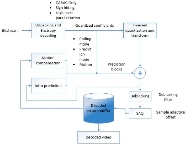
proposal: high-resolution video and parallel processing. Figure 2-9 shows the HEVC decoder structure, main including block segmentation, intra prediction, motion compensation, transform and quantization, deblocking, and sample adaptive offset (SAO).
Figure 2-9 HEVC video decoder processing.
2.7.3.
HEVC Coding structure
2.7.3.1.
Group of Pictures
The video sequence is composed of several consecutive frames, and when it is compressed, the video sequence is divided into several GOPs (Group of Pictures). GOP is divided into: closed GOP and opened GOP.
Closed GOP is shown in the following figure 2-10, each GOP begins with a IDR (Instantaneous Decoding Refresh), and each GOP is independently coded.
38
Figure 2-10 Closed GOP structure.
Open GOP is shown in figure 2-11, the first intra frame of the first GOP is an IDR frame, and the first intra frame in the subsequent GOP is a non-IDR frame [48]. That is, the inter frame in the subsequent GOP may cross the non-IDR frame and use the encoded frame in the previous GOP as the reference frame.
Figure 2-11 Opened GOP structure.
2.7.3.2.
Slices
Each GOP is divided into multiple slices which are independently encoded. This main purpose is to resynchronize in the event of data loss. Each slice consists of one or more slice segment (SS) [35, 49]. In HEVC, a slice contains only one fragment by default. That is a frame is a slice, but also a slice segment. Slices can be coded by applying different coding types [49]:
1. I slice: All coding blocks in I slice are intra prediction coded.
2. P slice: Coding blocks in P slice can be coded in both intra prediction and inter prediction with only one motion compensation signal.
3. B slice: Coding blocks in B slice can be coded in both intra prediction and inter prediction with one or two motion compensation signals.
39
2.7.3.3.
Tile
Tile is a new concept in HEVC. A frame can be divided into several slices, and it can be divided into several tiles, which divides an image from horizontal and vertical directions into several rectangular regions [36, 50]. The main purpose of tile division is to enhance the ability of parallel processing without introducing new error
diffusion. Tile provides a greater degree of parallelism (at the image or sub-image level) than CTB, without the need for complex thread synchronization. The division of tile does not require uniform distribution of horizontal and vertical boundaries and can be grasped according to the requirements of parallel computing and error control. In general, the CTU data contained in each tile is approximately equal. At the
encoding time, all tiles are processed in the order of scan. The number of CTUs in a tile and the number of CTUs in a slice does not affect each other. In the same image, some slices contain multiple tiles and some tiles contain multiple slices can
simultaneously exist.
Slice and tile are divided for the purpose of independent coding. The shape of the tile is substantially rectangular, and the shape of the slice is striped. A slice consists of a series of slice segments (SSs), a SS consists of a series of CTUs. Tile is directly composed of a series of CTUs.
2.7.4.
Prediction blocks
HEVC first divides a frame into a number of two-dimensional symmetric coding structure and then processing. CTU (Coding tree unit) [35] is the core of HEVC symmetric coding structure. CTU is similar with the "macroblock" in H.264 / AVC. The size of the CTU is not strictly limited. The size of CTU can be 64 × 64, 32 × 32, 16 × 16, and 8 × 8 [36]. The larger size can be better compression rate. CTU contains a luma CTB (Coding tree block) and two chroma samples CTBs. CTB cannot decide whether HEVC process intra or inter prediction. Thus CTBs can be partitioned into smaller blocks. CTU can be spilt into luma and chroma CBs (coding blocks). The
40
largest CU is called the LCU (Largest Coding Unit), the smallest CU is called the SCU (Smallest Coding Unit). The size of the LCU and SCU is generally limited to an integer power of 2 and normally greater than or equal to 8.
If the size of the LCU and the maximum depth of the recursive segmentation is known, the sizes of CUs in the LCU are known. If the size of the LCU is 64 × 64 and depth is 4, the CUs size can be 64 × 64 (LCU) [36], 32 × 32, 16 × 16, 8 × 8. If the LCU size is 16 × 16 and depth is 2 [70], the CU size is 16 × 16, 8 × 8.
Figure 2-12 CU quad-tree syntax.
The un-limitation size of coding block is conducive to improve the efficiency of HEVC. The coding blocks (CBs) can be divided into luma and chroma prediction blocks
(PBs). All the operations related to the prediction are processing in PUs. Intra mode difference, inter prediction, motion vector difference, reference frame index and motion compensation are based on PU processing. PU size is limited by the size of CU. After CU division, the size of PU is processing. There are three types of prediction mode in HEVC: Skip, Intra and Inter [50]. Predictive types are the main factors that affect PU segmentation. If the size of CU is 64 × 64, PU size is 64 × 64 in the skip mode. However, in intra mode, PU size may be 64 × 64 or 32 × 32. In Inter mode, PU size may be 64 × 64,64 × 32, 32 × 64, 32 × 32, 64 × 16, 64 × 48, 16 × 64 and 48 × 64 [37]. Residuals appear between the original blocks and its prediction blocks.
41
Figure 2-13 The block partitions in HEVC.
Residuals appear between the original blocks and its prediction blocks. The residuals of CBs can be split into smaller transform blocks (TBs). The size of transform blocks can be from 32*32 to 4*4.
HEVC also defines the TU (Transform Unit) as the basic unit of transformation and quantization. TU size may be greater than PU, but will not exceed the size of CU. TU must be two-dimensional symmetry. TU size is N × N or N / 2 × N / 2 [48] and depends on the PU split. The purpose of this segmentation design is to avoid TUs across the boundaries of PU. CU, PU, TU are independent and interrelated, this design is more in line with the texture features of images. Coding, prediction, transformation is more flexible [66] than H.264.
2.7.5.
Intra prediction
The intra prediction of HEVC is similar to H.264 / AVC. It is based on data from neighboring blocks to perform predictive reconstruction in various ways. When encoding high-definition video, larger coding units will be applied. In order to make the intra prediction more accurate, the prediction modes of HEVC brightness component up to 35. Including two non-directional predictions: DC and Planar, and another 33 kinds of directional prediction [38]. As shown in Figure 2-14, there are five prediction modes for chrominance components: horizontal, vertical, DC, DM (Derivation Mode) and LM (Linear Mode) [67], where the DM mode determines the chrominance prediction mode according with the luminance prediction mode. The LM
42
mode predicts the chromaticity of the current block based on the luminance and chrominance linear model relationships of neighboring blocks.
Figure 2-14 Intra prediction modes and directions of angular prediction. [58]
2.7.5.1.
Planar prediction Mode
The Planar prediction is suitable for reconstruction of smoothing content. The JCT-VC first proposes this prediction scheme. First, the lower right corner pixel of the block is written to the coding, and then interpolates the rightmost column and the bottom row according to the adjacent block reconstruction pixel. The predictions of other pixels are obtained by bilinear interpolation. In 2011, JCT-VC proposes another planar prediction method [39]. The pixel at the bottom right corner is interpolated by the adjacent blocks instead transmission to the decoding part. In addition, the bilinear interpolation is changed to the average of horizontal and vertical linear interpolation.
2.7.5.2.
Linear Mode (LM) prediction
LM (linear model) is new chroma prediction mode in HEVC. The specific calculation of chroma prediction is:
43
𝑃𝑟𝑒𝑑𝑐[𝑥, 𝑦] = 𝛼. 𝑅𝑒𝑐𝑙′[𝑥, 𝑦] + 𝛽 (2-16)
Where 𝑃𝑟𝑒𝑑𝑐[𝑥, 𝑦] is the chrominance prediction signal of the current block, 𝑅𝑒𝑐𝑙′[𝑥, 𝑦] is the luminance reconstruction signal of the current block. 𝛼 and β are derived from the relationship between the luminance and chrominance signals of adjacent blocks.
If the video source is in YUV 4: 2: 0 format, the sampling rate of the chrominance signal is half that of the luminance signal. When using the LM prediction, the chrominance and luminance signals have a phase difference of 1/2 pixel. Therefore, it is necessary to first sample the luminance signals to match the size and phase of the chrominance signals. In the LM prediction mode, the reconstructed luminance signals down sampled in the vertical direction, and secondary sampled in the horizontal direction:
𝑅𝑒𝑐𝑙′[𝑥, 𝑦] = (𝑅𝑒𝑐𝑙[2𝑥, 2𝑦] + 𝑅𝑒𝑐𝑙[2𝑥, 2𝑦 + 1]) ≫ 1 (2-17)
By using least squares method, the relationship between the reconstructed luminance signal and the chrominance signal after the down sampling can be fitted to derive the parameters α and β. 𝛼 =𝐼 ∑𝐼𝑖=0𝑅𝑒𝑐𝑐(𝑖)𝑅𝑒𝑐𝑙′(𝑖)−∑𝐼𝑖=0𝑅𝑒𝑐𝑐(𝑖)∑𝐼𝑖=0𝑅𝑒𝑐𝑙′(𝑖) 𝐼 ∑𝐼 𝑅𝑒𝑐𝑙′(𝑖)𝑅𝑒𝑐𝑙′(𝑖)− 𝑖=0 (∑𝐼𝑖=0𝑅𝑒𝑐𝑙′(𝑖))2 =𝐴1 𝐴2 (2-18) 𝛽 =∑𝐼𝑖=0𝑅𝑒𝑐𝑐(𝑖)−𝛼∑𝐼𝑖=0𝑅𝑒𝑐𝑙′(𝑖) 𝐼 (2-19)
𝑅𝑒𝑐𝑐(𝑖) 𝑎𝑛𝑑 𝑅𝑒𝑐𝑙′(𝑖) represent reconstructed chrominance signals and
reconstructed downsampled luminance signals. I is the total number of adjacent block sampling points.
Only the left and upper sides of the current block are sampling points. In the Intra configuration, LM mode enabled to increase the BD-rate of 𝑌, 𝐶𝑏 and 𝐶𝑟 by 0.8 %, 7.8% [51] and 5.9% [52].
2.7.6.
Inter prediction
As the PU segmentation may use four kinds of asymmetric way (2N × nU, 2N × nD, nL × 2N, nR × 2N), the motion vector is also allowed to asymmetric block as a unit in
44
the inter prediction. This technique is called AMP (Asymmetric Motion Partition). The asymmetric shape of the region can be more flexible for motion estimation.
Conventional video encoders generally use predictive coding for motion vector coding. In addition, the difference between the MV prediction value and the actual value is encoded [40]. This spatial motion vector predictive coding method is also known as MVP (Motion Vector Prediction).
AMVP (Advanced motion vector prediction) is proposed instead of MVP in HEVC. The motion vector prediction candidate blocks are not limited to the spatial domain, also within the time domain. These candidate blocks to form a collection. The AMVP scheme will find the optimal MV matching in this collection, and then encoding the index of the optimal matching block, reference frame subscript, and MVD (Motion Vector Difference), so as to save the space cost more effectively. If MVD is 0, HEVC will enable the merge mode so that the current block and the candidate block share a motion vector. HEVC generally uses both AMVP and merge to achieve optimal MVP encoding efficiency.
2.7.7.
Transform and quantization
2.7.7.1.
Large scale Transform
H.264 / AVC only contains 4 × 4 and 8 × 8 transformation modes. HEVC added 16 × 16, 32 × 32 two large scale transformation [65]. For HD video, the use of large scale frequency domain transformations will achieve better coding result. Because blocks represent content that is typically part of a particular object or a small portion of the background in HD video, the contents of blocks are mostly uniform texture patterns and subtle color changes. The calculation [41] can be expressed as:
45 𝐻 = [ 64 64 64 64 64 64 64 64 64 64 64 64 64 64 64 64 90 87 80 70 57 43 25 9 −9 −25 −43 −57 −70 −80 −87 90 89 75 50 18 −18 −50 −75 −89 −89 −75 −50 −18 18 50 75 89 87 57 9 −43 −80 −90 −70 −25 25 70 90 80 43 −9 −57 −87 83 36 −36 −83 −83 −36 36 83 83 36 −36 −83 −83 −36 36 83 80 9 −70 −87 −25 57 90 43 −43 −90 −57 25 87 70 −9 −80 75 −18 −89 −50 50 89 18 −75 −75 18 89 50 −5 −89 −18 75 70 −43 −87 9 90 25 −80 −57 57 80 −25 −90 −9 87 43 −70 64 −64 −64 64 64 −64 −64 64 64 −64 −64 64 64 −64 −64 64 57 −80 −25 90 −9 −87 43 70 −70 −43 87 9 −90 25 80 −57 50 −89 18 75 −75 −18 89 −50 −50 89 −18 −75 75 18 −89 50 43 −90 57 25 −87 70 9 −80 80 −9 −70 87 −25 −57 90 −43 36 −83 83 −36 −36 83 −83 36 36 −83 83 −36 −36 83 −83 36 25 −70 90 −80 43 9 −57 87 −87 57 −9 −43 80 −90 70 −25 18 −50 75 −89 89 −75 50 −18 −18 50 −75 89 −89 75 −50 18 9 −25 43 −57 70 −80 87 −90 −90 −87 80 −70 57 −43 25 −9 ]
2.7.7.2.
Alternative DST
For 4 × 4 size TU, HEVC provides an optional DST based transformation mode. The transformation matrix is shown as below:
𝐻 = [ 29 55 74 84 74 74 0 −74 84 −29 −74 55 55 −84 74 −29 ]
DST has better coding adaptability for regions that the residual amplitudes increased. And DST can save about 1% of the bit rate [42]. In addition, DST conversion is only used to 4 × 4 luma transform blocks.
2.7.7.3.
Transform Skipping
In order to improve the efficiency of video coding, HEVC also involves some other coding techniques. TSM (Transform Skip Mode) [43] is one of the technologies adopted by HEVC. Due to the anisotropic characteristics of video content, the traditional Hybrid video encoder cannot achieve the best coding results. It will be better to encoder prediction residual directly without frequency transformation.
Since the correlation between blocks of intra prediction is not as high as inter prediction, the prediction residual of intra prediction is generally large, especially for coding blocks.
46
The use of 2D frequency domain transforms facilitates energy concentration [42,43]. If the video source is a screen image, the content is mostly repetitive lossless matching data, the intra prediction residuals will be smaller or zero, in which case if the frequency domain transform is still used, it will be reduced coding efficiency. In this case, transform units will skip the transformation in TSM. In the subsequent CABAC entropy coding stage, the statistical properties of residual data can be modified to obtain better coding results.
The motion compensation residual signal generally exhibits different characteristics in both vertical and horizontal directions. Therefore HEVC can select different TSM [44] to skip the horizontal/vertical transform according to the specific situation in inter prediction. The TSM mode also includes the option of enabling both horizontal and vertical transformations. For some screen videos, BD-rate performance can be increased by up to 30% after enabling TSM with less modification to HEVC encoder.
2.7.7.4.
Quantization
The processing of quantization is to obtain a simpler representation of the transform coefficients. Quantization is the main reason of distortion in compression, so choosing the appropriate quantization step size to balance distortion and bit rate becomes the key problem. The quantization step size in HEVC is marked by the quantization parameter (QP), with a total of 52 levels (0 to 51). Each QP corresponds to an actual quantization step size. The large value of QP means the quantization will result in the lower bit rate, and the greater distortion will be. HEVC uses the Rate Distortion Optimized Quantization (RDOQ) technique to select the optimal quantization parameter for a given bit rate to minimize the distortion of the reconstructed image.
47
2.7.8.
In-loop filtering
2.7.8.1.
Deblocking Filter
Due to the error caused by the quantization of the frequency domain transform and the prediction deviation caused by the motion compensation, the block based coding processing appear effect that PU and TU boundaries are not aligned after the deblocking Filter prediction/transformation/quantization step. Therefore, the hybrid video encoder will eliminate that effect. The general practice is adding deblocking filter in the block boundary [45]. HEVC to block filter basically follows the H.264 / AVC method [64], such as filtering method and boundary strength decision mechanism. The only difference is that HEVC adopted More flexible block segmentation s


![Figure 2-14 Intra prediction modes and directions of angular prediction. [58]](https://thumb-us.123doks.com/thumbv2/123dok_us/776236.2598152/43.892.251.639.180.564/figure-intra-prediction-modes-directions-angular-prediction.webp)