Stereo Vision Algorithms
Stian Selbek
Algorithms
Stian Selbek
The process of stereo vision matches one or more images to recover the depth information of the pictured scene. Great progress is currently being made within this field, with algorithmic research, computational power developments, and cheaper cameras all contributing to give stereo vision great future potential as the depth measuring system of choice. One of the challenges of the stereo vision approach is the multitude of control parameters, which all affect algorithm behaviour. These parameters have traditionally been tuned by hand, with some limited use of computerized optimisation techniques. However, the process of evolutionary computation provides a promising method of optimisation of such complex problems.
This thesis explored the possibility of applying a multi-objective evol-utionary optimisation approach to the stereo algorithm parameter prob-lem. In this regard, an automatic parameter optimisation framework based on the multi-objective optimisation algorithm NSGA-II was developed and tested.
In order to judge the performance of the framework and the validity of the multi-objective approach, three different stereo algorithms were tested and a series of near pareto-optimal parameter sets were produced. One parameter set per algorithm was submitted to the official KITTI stereo vision benchmark ranking, and was able to improve upon the current official results.
I wish to thank my two supervisors, Kyrre Glette and Johannes Solhusvik for their inspiration and help. With your assistance I was able to explore a new and exiting field.
I would also want to thank Andreas Geiger of MPI Tübingen for his assistance with the KITTI benchmark submission process.
Lastly, I want to thank my fellow students, family, friends, and the staff at the ROBIN group for their support.
1 Introduction 1
1.1 Goals . . . 2
1.2 Thesis Outline . . . 2
2 Background 3 2.1 Stereo Vision . . . 3
2.1.1 Epipolar Geometry and Rectification . . . 4
2.1.2 Stereo Correspondence . . . 5
2.1.3 Sparse Stereo Correspondence . . . 6
2.1.4 Dense Stereo Correspondence . . . 7
2.1.5 Post Processing . . . 10
2.1.6 Comparison to other ranging techniques . . . 11
2.2 Stereo Algorithms . . . 12
2.2.1 Evaluation of Algorithms . . . 12
2.2.2 OpenCV Block Matching (BM) . . . 15
2.2.3 OpenCV Semi Global Block Matching (SGBM) . . . 17
2.2.4 ELAS - Efficient LArge-scale Stereo . . . 17
2.3 Evolutionary Algorithms . . . 18
2.3.1 An Introduction to Genetic Algorithms . . . 19
2.3.2 Evolutionary Multiobjective optimisation . . . 22
2.3.3 NSGA-II - Non-dominating Sorting Genetic Algorithm 25 2.4 Tools . . . 26
2.4.1 Statistics . . . 26
2.4.2 The OpenCV library . . . 28
2.4.3 TBB - Intel Threading Building Blocks . . . 28
3 Implementation 31 3.1 An Overview of the Evolutionary Framework . . . 31
3.2 The Evaluation Method . . . 32
3.2.1 Choice of Data Set . . . 32
3.2.2 Disparity Calculation . . . 33
3.2.3 Disparity Evaluator . . . 35
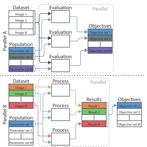
3.2.4 Evaluation Computation Strategies . . . 36
3.2.5 Timeout methods . . . 38
3.2.6 Uniqueness Constraint . . . 39
3.3 Evolutionary Setup . . . 41
3.3.2 NSGA-II . . . 42
3.3.3 Setting the crowding distance type . . . 43
3.3.4 Selection, Mutation and crossover . . . 44
3.3.5 Added and changed features . . . 44
3.3.6 Run Setup and Worker Assigments . . . 45
3.4 The Stereo Algorithms . . . 46
3.4.1 Genome . . . 47
3.4.2 Setting the Parameter Limits . . . 47
3.4.3 Additional Prefiltering . . . 48
3.5 Population Validation . . . 50
3.5.1 The N Best Out Percentage Method . . . 51
3.5.2 The Online Pareto Front Method . . . 51
3.5.3 The Offline Pareto Front Method . . . 51
4 Experiments & Results 55 4.1 Experiments on the Implementation . . . 55
4.1.1 Parallel Evaluation methods . . . 56
4.1.2 The Effect of Training Set Size . . . 59
4.1.3 Testing objective functions and helper objectives . . . 62
4.1.4 Real-time and CPU-time methods . . . 64
4.1.5 The Uniqueness Check . . . 67
4.2 Multi-Objective Parameter optimisation . . . 69
4.2.1 Quality, Density and Hypervolume . . . 70
4.2.2 Parameter Distribution . . . 73
4.2.3 Runtime Results . . . 76
4.2.4 Comparison with single-objective optimisation . . . 77
4.2.5 Results on Near Real-time Individuals . . . 80
4.3 A Brief Look at Overfitting and Generational Progress . . . 83
4.3.1 Results . . . 83
4.3.2 Analysis . . . 85
4.4 Results With Prefiltering . . . 85
4.4.1 Results . . . 86
4.4.2 Analysis . . . 90
4.5 The Timeout Threshold . . . 92
4.5.1 Results . . . 93
4.5.2 Analysis . . . 95
4.6 Improving on the Results . . . 95
4.6.1 Results . . . 96
4.6.2 Analysis . . . 98
4.7 Submitting Results to the KITTI benchmark . . . 100
4.7.1 Results . . . 101
4.7.2 Analysis . . . 102
5 Discussion 105 5.1 General Discussion . . . 105
5.1.1 Evolutionary Multi-Objective Optimisation . . . 105
5.1.2 The Framework as a Design Tool . . . 106
5.3 Future Work . . . 107
Bibliography 111 Appendices 119 A Algorithm parameter ranges 121 B Datasets 125 B.1 Training . . . 125
B.2 Test . . . 125
B.2.1 Testset A . . . 125
B.2.2 Testset B / Validation set . . . 125
C Additional Data Tables 127 C.1 Timeout Methods . . . 127
2.1 A Typical Binocular Stereo Vision Setup . . . 3
2.2 Epipolar Geometry . . . 5
2.3 Disparity to Depth comparison . . . 6
2.4 Sparse Stereo Correspondence . . . 7
2.5 Disparity Space Image . . . 8
2.6 Lidar point cloud . . . 11
2.7 BM and SGBM prefilters . . . 16
2.8 ELAS support points . . . 18
2.9 Overview of a Typical Genetic Algorithm . . . 19
2.10 The Two-Point Crossover Operator . . . 21
2.11 Pareto-optimal Solutions . . . 23
2.12 The 2D Hypervolume . . . 24
2.13 NSGA2 Structure . . . 25
2.14 Illustrated Boxplot Example . . . 27
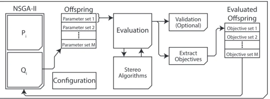
3.1 Implementation Overview . . . 31
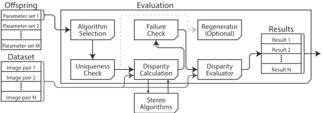
3.2 Evaluation Overview . . . 32
3.3 Example KITTI dataset images . . . 34
3.4 Parallel Evaluation Strategies . . . 37
3.5 No Timeout Method Illustration . . . 38
3.6 Uniqueness Checker . . . 40
3.7 Bad Objective Threshold . . . 42
3.8 Soft non-dominated sorting . . . 45
3.9 Worker Assignment Techniques . . . 46
3.10 Appending the Prefiltering genome limits . . . 49
3.11 Workflow of the Offline Pareto Front Method . . . 52
3.12 Post Run Pareto Front Extraction . . . 52
3.13 Pareto Front Reduction . . . 53
4.1 Comparing computational strategies . . . 58
4.2 Training set size results . . . 60
4.3 Boxplot of Timekeeping Methods . . . 65
4.4 Rank Outliers of Timekeeping Methods . . . 65
4.5 Results on the Uniqueness Checker . . . 69
4.6 Pareto front of Bad versus Invalid . . . 71
4.7 Pareto front of Bad versus Invalid - Transferability . . . 71
4.8 Hypervolume of Bad vs Invalid Fronts . . . 74
4.10 Runtime Analysis of Pareto Front . . . 77
4.11 Parameter Analysis on the runtime of the Pareto Front . . . . 78
4.12 3D histogram of objective space . . . 79
4.13 Pareto Front of Bad vs Invalid - Sub 1s Solutions . . . 82
4.14 Boxplot of Sub 1s Solutions’ Runtime . . . 82
4.15 Plot of hypervolume over time . . . 84
4.16 Analysis of Loss in Hypervolume . . . 86
4.17 Hypervolume of BM with Additional Prefiltering . . . 87
4.18 Time used on each prefilter for BM . . . 87
4.19 Hypervolume of ELAS with Additional Prefiltering . . . 88
4.20 Time used on each prefilter for ELAS . . . 88
4.21 Hypervolume of SGBM with Additional Prefiltering . . . 89
4.22 Time used on each prefilter for SGBM . . . 89
4.23 Analysis of Additional Prefiltering Techniques . . . 91
4.24 Boxplot of hypervolume for the timeout methods . . . 94
4.25 Boxplot of time used for the timeout methods . . . 94
4.26 Combined pareto fronts . . . 97
4.27 Boxplot of hypervolume . . . 97
4.28 Parameter analysis for the last experiment - algorithms . . . . 99
4.29 Parameter analysis for the last experiment - prefilters . . . 99
4.30 SGBM search space problem . . . 100
2.1 List of Software Used . . . 26
3.1 Comparison of Computation Strategies . . . 36
3.2 List of prefiltering types . . . 48
4.1 Runtime of evaluation methods . . . 57
4.2 Training Set Size Experiment Setup . . . 59
4.3 Training set size results . . . 60
4.4 Training Set Size Experiment Setup . . . 62
4.5 Results of the Objective Type Experiment . . . 62
4.6 Objective Type Comparison . . . 63
4.7 Timekeeping experiment setup . . . 64
4.8 Runtime Distribution among Timekeeping Methods . . . 66
4.9 Table of Uniqueness Checker Results . . . 68
4.10 Initial Pareto Front Experiment Setup . . . 70
4.11 Comparison with algorithm defaults . . . 72
4.12 Potential quality-density trade-offs . . . 73
4.13 Parameter Repeat Counts . . . 75
4.14 Near Real-Time Results . . . 81
4.15 Front Size Comparison After Change in Objectives . . . 84
4.16 Runs and runtimes for the Prefiltering Experiments . . . 90
4.17 Setup for the Timeout method experiment . . . 92
4.18 Final Pareto Front Experiment Setup . . . 95
4.20 Total Hypervolume Comparison . . . 98
4.21 Updated quality-density trade-offs . . . 98
4.22 KITTI - Individuals to submit . . . 102
4.23 KITTI - Results Table . . . 102
A.1 BM parameter range . . . 122
A.2 ELAS parameter range . . . 123
A.3 SGBM parameter range . . . 124
B.1 The Training Data Sets . . . 125
B.2 The Test Data Sets . . . 126
C.1 Timeout Methods - Wilcoxon Ranksum . . . 127
C.2 Submitted BM Individual . . . 128
C.3 KITTI BM test result . . . 129
C.5 KITTI ELAS test result . . . 131 C.6 KITTI SGBM test result . . . 132 C.7 Submitted SGBM Individual . . . 133
Introduction
The field of computer stereo vision allows 3D depth information to be extracted from two or more partially overlapping images. This technique has found use in many areas including robotic exploration [21], planetary [57] and solar observation [37], autonomous cars and driver assistance applications [56], and video conferencing, among others. Yet rapid development in stereo algorithmic research, cheap consumer cameras and the computational power required to calculate the results, all point to the even greater potential inherent to this technique in the years to come.
However, a common issue with stereo algorithms is the difficult tuning of their algorithm control parameters, which all modify their specific behaviour. These parameters are typically tuned by hand by altering them in turn, thereby garnering a better idea of their effect on the resulting output. This is a slow and laborious process and that makes it difficult to account for both multiple parameters at once, and their possible inter-dependence and effect. Fast, near real-time stereo algorithms present the practical opportunity to use computational optimisation methods to automatically tune algorithm control parameters to maximise quality on example images over the course of thousands of evaluations. Some work has been done in this regard using common statistical optimisation methods [85], but these tend to require a representative statistical model for minimization. Other alternatives include grid search, which performs a limited exhaustive search, and is thus a computationally expensive technique.
Evolutionary algorithms, inspired by the natural process of evolution, may provide a promising possibility for stereo parameter optimisation. This optimisation strategy is able to find near-optimal solutions with comparatively simple steps, even in large unknown problems. Some examples include the evolution of virtual creatures [70], component design [9], job scheduling [7], path planning [35], or even stereo vision [22]. However, only limited work has been published in this area in regards to actual stereo parameter optimisation, and then only with an optimisation of a single quality objective [53, 73].
1.1. GOALS
1.1
Goals
With the increased popularity of multi-objective optimisation techniques, this presents a good opportunity to test the possibility of using such a method on the computer stereo vision parameter optimisation problem. As such, the first goal of this thesis will be the implementation of a robust framework capable of parameter optimisation of stereo algorithms.
As a second goal, the possibility of using a multi-objective approach for algorithm parameter optimisation shall be investigated. This entails optim-ising several stereo algorithms to see if the multi-objective focus provides a feasible method for optimisation. Of particular secondary interest is the promising ability of a multi-objective approach to not only adapt paramet-ers to different trade-offs, but also to compare stereo algorithm perform-ance along their entire pareto fronts, giving the possibility of a more de-tailed view than traditional stereo algorithm comparisons.
1.2
Thesis Outline
This thesis is divided into five chapters with each dedicated to a certain aspect of the project. Beyond this introduction, the thesis starts with relevant background material presented in Chapter 2. This gives an overview of the computer stereo vision process, its different methods and certain algorithms relevant to the thesis. Background information in evolutionary algorithms with a focus on genetic algorithms and multi-objective optimisation is also covered in this chapter.
Chapter 3 describes the implementation of the stereo parameter optim-isation framework and how its various modules operate. In Chapter 4 the experiments done to tune the details of the framework for more robust res-ults is first presented. Then the framework is used to explore the possibility of improving on current benchmark results. Lastly Chapter 5 discusses the performance of the framework and the results acquired through its use. This chapter also contains the conclusion and a presentation of possible future work.
Background
This chapter contains relevant background information to the thesis. First, Section 2.1 provides an introduction to stereo vision with a focus on the faster variants most relevant for use in evolutionary computing. A sample of stereo algorithms is described in more detail in Section 2.2, in addition to a review of how algorithms may be compared. Then an introduction to the concepts of evolutionary computing with a focus on genetic algorithms is done in Section 2.3. Lastly tools used in this thesis are presented in Section 2.4.
2.1
Stereo Vision
Stereo vision is the art of extracting depth from images by comparing two or more partially overlapping pictures taken from slightly different perspectives. The typical binocular setup takes inspiration from the human vision system and includes two horizontally displaced cameras in the same plane as shown in Figure 2.1.
Figure 2.1: Binocular stereo vision process showing a typical camera rig, the left and right images as perceived by it, as well as two possible ideal colour-mapped depth representations of the input.
2.1. STEREO VISION
To illustrate how depth can be extracted from such a setup, said human vision system can serve as a practical example. Look at items at various distances while closing each eye alternately then note how objects will appear to jump left and right with moves inversely proportional to the distance to said feature [50]. By collecting these jumps, ordisparities, for each point in the image we get the disparity space [49] of said image pair which we can refine into a proper depth map of the scene. While this simple test gives the impression of simplicity, actually finding the same match in the computer stereo vision case is a more complicated task and may not even be possible at all if the object is partiallyoccluded, meaning it is only visible in one image.
In this section an introduction will be made to some stereo vision concepts, starting with camera requirements, then moving on to the actual matching step with a presentation of some common methods. Last a comparison with other ranging techniques is done.
2.1.1 Epipolar Geometry and Rectification
The practical experiment of Section 2.1 worked because the brain is able to correct for the relative placement of the eyes and their individual orientation. After this correction, object disparities in this example were limited left and right movement due to the horizontal alignment of the eyes. This camera correction process will need to be transferred to the case of two cameras before a proper matching step can begin. Without it the images would not be aligned, and the computer would have to search across the entire other image for each point it attempts to match, which would be a very time consuming process.
A point seen by a single camera only describes the projection of that point to the camera plane. The point itself can exist anywhere along a projected line in that direction as no depth is implied by just this point. The concept ofepipolar linesdescribes how this projected line is viewed within the image plane of a different observing camera as shown in Figure 2.2. What this concept means is that when a computer lacking the human image context is to make a match, it no longer has to scan the entire other image looking for the best candidate, but can instead simply scan along this epipolar line. To find that particular line we must know the camera geometry or recover it from common points in the image [84]. A simplifying approach is to attach the cameras in the same plane with aligned horizontal lines. This mostly aligns the epipolar lines and forms the basis for the traditional horizontal stereo camera rig of Figure 2.1.
To increase the accuracy of the matching it is important to properly calibrate the rig by applying a transform to each camera and thereby aligning the image rows to each other projected to a common plane. This calibration, or rectification, can take many forms, but the resulting transform is typically solved by first photographing a known planar pattern at multiple angles then calculating the pose and distortion of each camera [83]. This process causes some image distortion along the edges which reduces the effective image size depending on how well aligned the cameras
A
B
A
B
A
A
B
B
Figure 2.2: Searching for an object marked by the star in different camera geometries. The images as perceived by the cameras are on the right while the geometry is on the left. Note how matching can be done by only looking along the dotted lines and how the parallel binocular setup simplifies rectification.
were before rectification.
Before stereo calibration can occur it is important that slightintrinsic variation in the different cameras is compensated for as otherwise the same object may look inherently different in the two images making matching difficult. In this regard one must account for lens distortion and can expect sensor noise and exposure levels to vary even with sensors of the same make and model.
2.1.2 Stereo Correspondence
Stereo correspondence is matching points in one image with their corres-ponding point in the other within the region of camera overlap. This allows disparities to be calculated, and given the camera focal length and indi-vidual pixel size, the disparities can be related to depth via Equation (2.1). This gives a greater resolution at close range, as seen in Figure 2.3.
Dep t h(x,y)= basel i ne∗f oc al
pi xel si ze∗d i spar i t y(x,y) (2.1) The matching process may initially sound simple, but how exactly can we be sure that point A in one image is really point B in the other? This is known as thecorrespondence problemand is made more difficult by areas of low texture, repetitive patterns, brightness differences and reflective surfaces. An example may include two horizontally aligned cameras looking at a bright white wall through an image row aligned picket fence with a shadow covering one of the cameras causing uneven brightness in the output images. How can we now be certain of which plank of the fence should match which in the other image? And for a computer based approach, how can we match a single pixel on that plank when all other
2.1. STEREO VISION 0 50 100 150 200 250 0 10 20 30 40 50 60 70 80 90
100 computed disparity to actual distance
pixel disparity
actual distance (m
)
L R
Figure 2.3: Example of the non-linear relationship between calculated disparity and actual depth. Exact relationship varies according to equation 2.1.
planks will have pixels matching it to some extent? In addition to this problem making a match should remove the matched point from future matches making the stereo correspondence problem NP-complete and in need of approximating solutions.
Two main paradigms are used to approach the stereo correspondence problem. The feature based sparse stereo methods match only the most certain points, while dense stereo methods use areas around each point to gather more information allowing more dense results to be had.
2.1.3 Sparse Stereo Correspondence
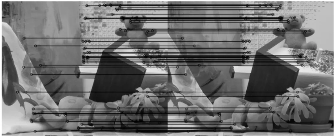
In computer stereo vision some points will be easier to match than others as they are easier to uniquely identify in the matching image. This opens the possibility of doingsparse stereo correspondencein which just the most robust features like edges, corners, or otherwise unique areas are matched between images. An example of this method can be seen in Figure 2.4. This leaves harder matches like low texture or ambiguous areas uncalculated, but region growing [24] and other surface fitting algorithms can be used to interpolate between these initial features. The advantages of the method lies in the high confidence answers on the feature points, even on imagery with differing illumination, as well as the limited computational effort required. Combined this led to early computer stereo vision work focusing on sparse correspondence methods.
Within the current field of stereo vision sparse correspondence with robust feature selection operators like SIFT [47], SURF [2], and FAST [64] remain useful for camera calibration [38, 83] and aiding dense stereo calculations [19]. Beyond these uses feature extraction has found use in related fields like finding road profiles, obstacles detection [45], face detection, mapping, and object recognition.
Figure 2.4: Example of sparse stereo correspondence using a feature extractor. Lines show the location of the point in both images. These locations can then be used to compute the disparity of that feature. Only the points with the most robust matches are kept, but what is construed as a good match can be tweaked to return more points at the cost of certainty of each new match. Made with OpenCV (see Section 2.4.2) using the FAST detector followed by a matching step. The Teddy image used is part of the Middlebury dataset [54].
2.1.4 Dense Stereo Correspondence
While sparse correspondence can find and identify points of interest, it is often useful for classification and tracking purposes to have a better segmented representation of the depth. The goal of dense stereo correspondenceis then to calculate the disparity of every pixel within the reference image. This requires much more computational power than sparse correspondence and proves more challenging as ideally every area must get an assigned depth, even areas of partial occlusion (hidden to one camera), low contrast, poor lighting, and areas of repeating textures.
To simplify matching a few assumptions are made in regards to how the world is to be perceived. Surfaces are assumed to beLambertian, this means that objects are assumed to have the same visual appearance in both images. In addition the world is assumed to consist of piecewise smooth surfaces [79]. These assumptions can be rewritten as an energy function E =mat chC ost+smoot hC ost. By minimizing this energy the goal of a stereo algorithm becomes finding the closest match while attempting to keep adjacent pixels at similar disparity. How the algorithm goes about this task is usually split into local and global methods.
As per Scharstein and Szeliski’s work [66], dense stereo correspondence usually do a subset of the following steps:
1. Pixel-based matching cost computation on pre-rectified input. For a given pixel this determines a similarity measure to all its possible matches. Across all pixels this creates a disparity space image(DSI) [34] as can be seen in Figure 2.5. Common similarity measures include absolute and squared difference, but while simple to compute
2.1. STEREO VISION Shift 0 Shift 1 Shift N Y X Y X Left image Right image
Disparity Space Image
Figure 2.5: Disparity Space Image (DSI) showing how the pixel marked in the left image (red) is matched in the right image. In this example matching starts in the same spot in the right image and shifts leftwards while computing a matching score each step of the way. This matching score is stored in the DSI and used to compute the final best match.
they are easily affected by sampling and illumination variance. More robust measures include Birchfield et al. [3], normalized cross-correlation [24] and the census transform [80], though the latter two combine their work with the next step.
2. Cost aggregation. Deciding on depth using the direct results of the previous step tends to be influenced by noise in the data. To reduce this influence and provide smoothness as in the assumptions earlier, cost aggregation will usually be done across a support region. The simplest of support regions would be a fixed size square window wherein the matching cost is summed or averaged. Better windows are available and will be discussed in Section 2.1.4 Local Methods.
3. Disparity computation/search. This step is all about deciding which of the many possible matches in the previous step happens to be the best representative of the real depth. This can be as simple as a local winner takes all approach, or a more advanced global optimisation of the earlier mentioned energy function.
4. Post-processing / Disparity refinement. After the pixel correspond-ence calculation it is useful to further clean up the results. This is the subject of Section 2.1.5.
Global Methods
Global methods formulate the stereo matching problem as an explicit energy minimization problem wherein minimization algorithms are used to reach a global minimum error. Most of this work is then done in the disparity search step using an error value based on some variant of the earlier cost and smoothness equation. Current minimization techniques includes belief propagation [13], graph cuts[5] and dynamic programming. These approaches have traditionally led to the most accurate stereo algorithms [54], but they are often too heavy on both computational resources and memory usage for real-time implementation [72]. This generally makes them poor choices for an evolutionary approach needing thousands of evaluations.
Local Methods
In contrast to the global methods, local methods do most of their work in the cost aggregation stage. A typical implementation will have a sliding support region looking for the closest pixel-wise match to the reference point. Common cost matching strategies include Sum of Absolute Differences (SAD) and Sum of Squared Differences (SSD), as described in Equations 2.2a and 2.2a. Here the pixel px has each of its potential disparites d computed by looking at the difference between its neighbourhood in the left image IL and the neighbourhood of the potential match in the right imageIR. Other matching cost methods include more real-world photometrically robust variants like normalized cross-correlation [24], and the census transform [80].
SSD(p x,d)= X i∈w i nd owp x [IL(xi)−IR(xi−d)]2 (2.2a) S AD(px,d)= X i∈w i nd owpx |IL(xi)−IR(xi−d)| (2.2b) Through the use of windows a certain smoothness is implied as it averages out the noise of the image. The actual choice of window size can however be difficult as windows need to contain enough texture to ensure a proper match yet be so small as to only contain pixels of the same depth. This particular problem has seen much recent research including multiple windows [23], adaptive weights [31], and adaptive window sizes [81]. The latter two change their effective window size either through adjusting the importance of each pixel or by growing and shrinking the window dynamically. By only including similar areas in the effective support region this more or less solves the traditional window size problem.
For local methods the global energy-function is only implicitly optim-ised through locally optimal choices within the support region. By the use of this window function only a limited area of the DSI is needed to calculate each result which makes local methods faster, more memory efficient and with easier parallelization than global methods.
2.1. STEREO VISION
In the disparity search stage the easiest solution is the Winner Takes All (WTA) strategy. This merely assigns the closest match as the disparity. While very easy to implement this technique doesn’t uphold uniqueness, that is a pixel in the non-reference image may actually end up mapped to several pixels in the reference image. This can lead to errors, but with a well-selected cost method results approaching the best global methods can still be achieved with the latest local algorithms.
A subset of the local algorithms are algorithms which while technically local still achieve behaviour similar to the global algorithms. Examples include cooperative algorithms [86] which are inspired by the human vision system wherein local computations are done iteratively, and hierarchical methods in which coarse initial results are used to guide increasingly detailed searches.
The most accurate local algorithms that still achieve real-time compu-tation are currently the Semi-Global Matching (SGM) of Hirschmuller [25] and the ADCensus [51] algorithm which uses many of the same building blocks. SGM achieves great results by optimising each point in at least 8, but ideally 16 or more directions using Dynamic Programming. The ori-ginal implementation uses a fair bit of memory, but a refined version which trades less memory usage for increased computing requirements, is avail-able [26].
2.1.5 Post Processing
Post processing disparity images allows potentially bad correspondence matches to be removed or replaced by better choices. This step may include aLeft-Right disparity checkin which the computed disparity referenced to one image is sanity checked by seeing if the selected match would end up with the initial pixel if correspondence was done in reverse. This cleans up the disparity output and can be used to detect occluded areas [17]. Other common operations includes a subpixel interpolation step in which the neighbouring disparity candidates to the best match are fitted to a function, e.g. a parabola, and then used to assign a more accurate subpixel resolution match. Often such post processing steps are included within the actual matching when the relevant information is available, this allows more efficient implementations by reducing memory access and removing such results at an early stage.
Other operations may include filtering the output disparity map via a mean or median filter. If done with care this will reduce noise and improve the quality of the results. Results interpolation may also be used to fill in small gaps in the output image, but used in large areas this may give false impressions in tasks where it is more important to know whether a result has been calculated with a degree of accuracy over giving the best approximate estimate available.
2.1.6 Comparison to other ranging techniques
Stereo vision is an inexpensive technique able to exploit the latest in small high resolution cameras. The sensors are passive and low power, offers no moving parts, high definition of the results, and with potentially high refresh rate. In addition they offer the additional option of using the same images for scene context, allowing e.g. signs, turn signals and brake lights to be analysed using the same hardware.
The main problems remain light variation, use in poor visibility, hardware requirements, and temporary solution degradation [33]. The following sections will provide a short introduction to sensors often used in parallel to, or instead of a camera rig.
Lidar
In autonomous vehicles an oft used method is the lidar, a laser based technique in which one or more beams of light are projected to the scene while a detector measures the time till the signal is reflected and returned. A typical 2D lidar configuration features one beam mechanically swept to get readings along that particular plane. More advanced, and expensive, 3D lidar models feature a column of beams all attached at slightly different angles to cover a larger vertical portion of the scene as the device is rotated. While rotating each return is recorded and optionally corrected for device movement before a point cloud is generated as in Figure 2.6. In this case the horizontal resolution is limited by the speed and accuracy of rotation as well as the bandwidth required for handling the number of points generated.
Figure 2.6: Lidar point cloud as generated from a single rotation of a Velodyne HDL-64E lidar unit mounted on a vehicle standing at an intersection. Points are colour-mapped based on the height of the obstacle from a low red to a tall purple. White contour lines are 10 meters apart. Image generated based on data from the Ford campus vision and lidar data set [60].
This approach provides excellent accuracy and ability to detect the presence of objects, but the limited vertical resolution and range-dependent horizontal resolution may make actual identification of objects difficult. For
2.2. STEREO ALGORITHMS
the decision-making process different decisions may have to be made based on whether an object is a post or a pedestrian, as different behaviours are assumed. This is usually solved with a sensor fusion approach in which the lidar data is either guiding or otherwise compared to camera data [63].
Lidar generally provides robust range finding and is unaffected by time of day as well as bright sunlight and otherwise varying lighting conditions. However as with a camera based range sensor lidar is affected by rain and snow, and may also report dust, fog and exhaust as a collidable objects [61, 76].
Radar
Radar is a widely used sensor, particularly in the automotive setting, were its seen use in cruise control [76], automatic collision avoidance, lane assistance, and parking assistance applications. A radio wave is transmitted and the return signal timed and analysed, allowing the range and target speed to be interpreted. The latter is through the Doppler effect and provides context to detected obstacles. If driving and an obstacle is in front of you it is rarely a problem if that car is moving the same direction.
Radar devices tend to be either fixed, which is very common with park-ing assistance sensors, or mechanically swept. A more recent development in the automotive field is the phased array radar which uses digital beam forming allowing the radar array to stay stationary yet still sweep a beam within a certain field of view. The primary benefits is the lack of moving parts and increased resolution. An interesting additional feature however is the ability to bounce a beam off the road surface allowing a look past the car ahead of the radar equipped vehicle.
While radars are weather independent they can still report spurious results. E.g. a car passing on a bridge far ahead, or in a different lane, may be reported as an actual obstacle. The resolution as such is fairly poor.
2.2
Stereo Algorithms
This section first explains how stereo algorithms can be rated and common evaluation data sets used. Lastly stereo algorithms used in this thesis are presented in some detail.
2.2.1 Evaluation of Algorithms
Stereo algorithms are typically evaluated by comparing the resulting disparity image with aground truth(GT) image. The ground truth image is a representation of the real underlying disparities as seen in the scene from one of the two camera viewpoints. In the case of computer generated test images this ground truth image can easily and accurately be created from the model of the scene. Computer generated images provide a controlled method for testing specific aspects of an algorithm, but may not represent all the nuances of a real-world stereo pair [75]. In contrast test images of lab
and especially outdoor scenes work well as general algorithm evaluators, but providing the ground truth of the visible scene requires a different approach as a 3D model and perfect knowledge of ones own position is rarely available.
One way to generate such a ground truth image is through the process known as structured light in which a series of patterns are projected to the scene while a camera captures how the pattern is distorted by visible objects [67, 68]. This creates highly accurate images, however, as the basic structured light technique relies on interpreting visible light from a projector, its accuracy is reduced both by distance and by ambient light diffusing the pattern. The number of patterns required for the best quality results and the multiple exposures of each also precludes scenes with movement. These limitations makes the method very well suited to lab and other static environments, but less suited for outdoor scenes.
For outdoor scenes a laser scanner approach is typically used in the form of a LIDAR (see Section 2.1.6). This produces a sparse point cloud of the scene which can then be translated to the viewpoint of the camera vision system and compared to the stereo correspondence results.
Quality Metrics
A number of metrics are used for comparing the output of the stereo algorithms with the ground truth. These measures typically compare the GT image and the result on a pixel by pixel basis. however, due to consistency checks and problematic regions even normally dense stereo algorithms (see Section 2.1.4) may produce areas with no set disparity level. Whether such pixels have been rejected or are simply uncalculated, they are nonetheless marked as invalid as per Equation (2.3b). Any calculated pixel may contribute to a number of error measures like the remaining Equations in 2.3. These are widely used in published results and benchmarks (see Section 2.2.1). EB ad= Phei g ht y=0 Pw i d t h x=0 (|d(x,y)−dGT(x,y)| >B adT hr eshol d) N (2.3a) EI nv al i d= Phei g ht y=0 Pw i d t h x=0 (d(x,y)==unmar ked) N (2.3b) EOut=EB ad+EI nv al i d (2.3c) EAv g B ad= Phei g ht y=0 Pw i d t h x=0 |d(x,y)−dGT(x,y)| Nmar ked (2.3d) ER M S= v u u t Phei g ht y=0 Pw i d t h x=0 |d(x,y)−dGT(x,y)|2 Nmar ked (2.3e) These metrics may be applied to the image as a whole or only in an area of interest. Applying a mask is useful for studying a particular quality in potentially problematic areas areas like partially occluded regions, low
2.2. STEREO ALGORITHMS
texture, or reflective areas. This in turn may give a better understanding of the particular strengths and weaknesses of each algorithm or indeed the parameters controlling it.
In addition to evaluating the resulting image, an important concern remains at what pace the result was calculated. This metric is more difficult to compare as the resulting time will not only depend heavily on the processor architecture and memory of that particular computer, but also on the actual implementation of the algorithm in question. As such comparisons can only be directly made within the same setup. Even so, runtime remains an important concern for real-time implementations and comparing the efficiency of algorithms. While it would be possible to compare the times spent directly, it is equally important to know how well an algorithm copes in regards to image size and the number of desired disparity levels. Such measures are included in the oft used measures of seconds per megapixel(s/MP) and themillion disparity levels per second (Mde/s) metric as per equations 2.4.
s/M P=t i me∗ 1000000
w i d t h∗hei g ht (2.4a)
Md e/s=w i d t h∗hei g ht∗d i spar i t i es
t i me ∗
1
1000000 (2.4b)
Stereo Datasets and Benchmarks
Good test data is required to get a handle on the performance of a stereo correspondence algorithm. Several datasets are currently publicly available, some of which are presented here.
The Middlebury dataset [54] originally created for the stereo taxonomy of Scharstein and Szeliski [66] has grown to become the de facto standard for testing stereo algorithms. It provides a series of stereo pair images as well as ground truth solutions describing the ideal disparity map for each part of the dataset. Algorithms are ranked based on their performance in normal non-occluded areas, performance near depth discontinuities and occluded areas. The results are publicly available along with links to the scientific papers of each algorithm.
While the Middlebury set provides an excellent driving force for research it has been shown that the lab ranking may not always match real-world performance [46]. This has lead to an increased focus on real-real-world problematic scenes with the desire for more robust results. The Middlebury benchmark is currently experimenting with a new updated dataset which includes such test scenarios.
The KITTI dataset [20] provides a number of real-world stereo images and sequences as recorded from a moving vehicle in Karlsruhe, Germany. The set is based on data from both greyscale and colour cameras, and is backed up by lidar provided ground truth as well as GPS and accelerometer data. When compared to the Middlebury set this real-world focus presents more of the potential problems a stereo algorithm may face in regards to noise and lighting conditions, which in turn should lead to more robust algorithms [18]. The dataset lays the foundations for the KITTI benchmark
and has found use in various autonomous vehicle related fields including stereo vision, optical flow and object recognition.
Beyond the datasets an important consideration remains the platform the implementation is to be used. In the case of a real-time implementation it is often required to simplify the algorithm to achieve the required throughput. Another concern may be how easily the algorithm can be parallelized for use in parallel hardware like graphics cards and programmable logic devices. Surveys on the applicability of algorithms in the real-time setting includes the work of Tippets et al. [72] and the more vehicle-oriented work of Mroz and Breckon [56], and Van der Mark and Gavrila [74].
2.2.2 OpenCV Block Matching (BM)
Block Matching as implemented in the OpenCV library (see Section 2.4.2) is a very fast stereo implementation based on the Small Vision System algorithm of Konolige [43]. BM is a purely local stereo correspondence algorithm which finds initial matches via small Sum of Absolute Difference (SAD) windows. As per Scharstein et al. [66] BM can be divided into initial matching, disparity optimisation and disparity refinement, with additional preprocessing of the input images.
Typically local window methods are sensitive to brightness differences in the image pair. The preprocessing step of BM includes image intensity normalization wherein the brightness of the images are adjusted by the mean intensity within local windows. An example of the output of this normalization approach can be seen in Figure 2.7b. Note how the box in the bottom right now has the same apparent intensity in both images. Also of note is the reflective surfaces in the image and how they still differ in appearance, making matching difficult.
The alternate and preferred preprocessing method of BM is the XSobel edge extractor (see Figure 2.7c). The goal of this prefilter is to extract more robust features for the matching step, and as edges tend towards stability within the image pair they make for a good choice. Matches are done horizontally, hence the Sobel filter is applied only in the X direction thereby highlighting edges crossing the epipolar lines. This implementation differs slightly from the original Konolige algorithm as originally a Laplacian on Gaussian (LoG) filter was used for combined smoothing and edge extraction.
The initial matching of the block matching algorithm is done using Sum of Absolute Difference (Equation (2.2b)) using a sliding window technique. Matches are however only assigned when there exists an acceptable amount of texture along the epipolar line direction. Additionally, for a match to be accepted it has to uphold a uniqueness constraint by being a certain ratio better than the second best match. Should this be in order a match is assigned and the disparity is calculated based on an interpolation between the neighbouring values giving 16 subpixel disparity resolution.
As a window based method the initial matching may have problems near object discontinuities as the window will contain parts of both the
2.2. STEREO ALGORITHMS
(a) The left and right input images
(b) The left and right image as adjusted by the normalized response prefilter
(c) The left and right image as output from the XSobel prefilter
Figure 2.7: The output of the normalized response filter (b) as implemen-ted in the Block Matching algorithm. XSobel prefilter (c) as implemenimplemen-ted in both BM and the Semi-Global Block Matching algorithms. Input images are cropped versions of the MotorcycleE image pair of the Middlebury benchmark [54]. This image pair features unequal brightness for robust testing. (prefilter size 9, prefilter cap 63)
background and the object. The background will also change from one image to the next due to perspective differences, which means that this issue may lead to potentially poor matches. BM compensates by carrying out a speckle removal step in which results within areas of large variation are removed. A left-right disparity check is also applied to further remove spurious matches.
2.2.3 OpenCV Semi Global Block Matching (SGBM)
The OpenCV Semi Global Block Matching algorithm is a blend of the BM algorithm (see Section 2.2.2) and Hirschmuller’s Semi Global Matching (SGM) [25]. Like the BM algorithm SGBM matches windows centred at each pixel with a uniqueness threshold applied. However, rather than the SAD metric a more accurate Birchfield Tomasi [3] cost metric is used. The XSobel prefiltering used by BM is incorporated into this matching step.
As with BM a uniqueness constraint is used to assist in good matches, but unlike BM a dynamic programming approach adapted from the SGM algorithm is used to improve the final matching. This variant is more limited than the one used in SGM and by default the dynamic programming is only used along rows to optimise the best disparity choice at each pixel. Inter-row consistency is not upheld by dynamic programming, but rather by a greedy approach. This mode, called the 5-way dynamic programming mode, allows the result to be computed in a single pass thereby greatly increasing the throughput over the SGM algorithm. An alternative slower two-pass version using 8-way dynamic programming is selectable through a control parameter. As with BM a subpixel interpolation step is done to increase the resolution of the resulting disparity.
The left-right check is handled within the disparity selection, and a median blur is applied to the end result. Lastly a speckle filtering step, as in BM, helps improve the accuracy of the result.
2.2.4 ELAS - Efficient LArge-scale Stereo
The Efficient LArge-scale Stereo (ELAS) algorithm by Geiger et al. [19] is a local method guided by robustly matched support points taking advantage of how some points are more easily matched than others. ELAS first applies a sparse grid across the image, then for each intersection a potential support point check is carried out. A point is a potential support point if the best match found in the other image is at least a factorτbetter than the next best match. Before such potential support points can become actual support points for the next step in the algorithm, the following refinement steps are done:
1. A left/right-consistency check must be successfully carried out within a threshold.
2. Potential support points which disagree with their immediate neigh-bours are removed as inconsistent points.
2.3. EVOLUTIONARY ALGORITHMS
3. When multiple points lie on a straight line, only the ends are kept as the points are deemed redundant and would interfere with the triangulation of the next step.
Figure 2.8: An example of the Delaunay triangulated support points of the ELAS algorithm using its Middlebury default parameters. The background image is the Teddy image of the Middlebury benchmark [54]. With the support points created the next step of the algorithm is to create a mesh based on these points so that the local search can be guided in an efficient manner. An intermediate flat mesh based on the support point image coordinates alone, is created via Delaunay triangulation. The Delaunay process defines triangles between all points while maximizing the minimum angle of each triangle. Figure 2.8 shows an example output from this process. Once this mesh has been created support planes are created between the support points with their Z-axis defined by their calculated disparities.
The generated planes are used in the matching step to greatly reduce the disparity search space based on the assumption of piecewise smooth disparities. By combining multiple planes more certain matches are generated. As with the support points a left-right disparity check is also used for more robust matching.
Built in post-processing includes speckle removal, result interpolation, and bilateral mean and median disparity filtering.
2.3
Evolutionary Algorithms
Evolutionary algorithms is a class of generate and test optimisation algorithms inspired by the biological process of evolution. The basic
premise is a population of candidate solutions to a problem, tested and rated on data relevant to the optimisation. Then a survivor of the fittest procedure, in the form of asurvivor selectionstep wherein good solutions are kept and bad ones potentially discarded, is carried out. The selection of the remaining candidates are combined to form new offspring and the process repeats giving a steadily increasing total population score, or fitness.
Unlike an exact solution an evolutionary approach does not guarantee that the global best solution to a problem is found. However, with good methods and testing procedures, good solutions can be found even on unknown problems without having to negotiate the entiresearch spaceof candidate solutions.
2.3.1 An Introduction to Genetic Algorithms
This section will focus on the Genetic Algorithm (GA) as described by Holland [29, 30]. Genetic algorithms are a popular subset of Evolutionary Algorithms and likewise work in an iterative process on a population of candidate solutions. The basic outline of such an approach is illustrated in Figure 2.9. Population Initialization Population Evaluation Parent Selection Parents Crossover / Mutation Offspring Survivor Selection Stop? No Yes
Figure 2.9: An overview of the flow within a typical genetic algorithm. Before the process can start the problem to be optimised will need to be represented in a way compatible with the GA and its operators. This takes the form of mapping problem specific parameters into a gene format representing thegenotypefor each individual. Problem parameters may be represented using a traditional binary representation, integer, or real-value representations among others. Running this genotype through the problem at hand creates thephenotyperepresentation for that individual and can be used toevaluateits performance. Evaluating the performance is done by afitness function which assigns a score based on how well the individual performed the task represented by the problem.
2.3. EVOLUTIONARY ALGORITHMS
can be started by creating a random initial population or by inputting values of interest to guide the search to that region of the search space. With this done the population is evaluated by the fitness function and each individual is assigned afitnessscore. The GA then proceeds to its main program loop starting with parent selection, which will be the subject of the next section. Parent Selection
At the start of each generation parent selection is applied to select the best individuals for creation of new offspring. The traditional approach is to select two parents, but multiple can also be selected [12]. Many methods exist, but most of them prioritize high fitness parents, while a random element ensures that a diverse set of parents are selected and thereby giving the best possibility of advancing the search through new offspring created through the genetic diversity operators ofcrossoverandmutation.
Example selection operators include fitness proportional selection wherein each candidate solution is assigned a portion on a roulette wheel proportional to its fitness, then the dice is cast and parents selected. The popular tournament selection works by selecting t random individuals then making a parent of the one with best fitness. The basic version uses a tournament of size 2, but larger tournaments may be used if a greater degree of selection pressure is desired. This process continues until the requisite parents have been found. This method implicitly ranks the population without requiring knowledge of the current fitness values of the entire population [4].
The Crossover Operator
Crossover is a genetic operator wherein two or more parents create one or more offspring by combining their genetic material according to specific crossover rules. The goal of this recombination process is to combine good parents in the hope of creating new even better offspring exploring new areas of the search space. Whether the operator is applied is controlled by a crossover rate parameter giving the probability that new offspring is generated or the parents themselves kept directly. The latter describes stationary crossover while the former will either become a contracting or expanding crossover depending on the parameters. Contracting and expanding refers to whether the offspring gene is generated between the corresponding parent genes or outside of them respectively.
Among the simplest forms of this operator is theone-point crossover. Given two parent genomes it generates two offspring by first selecting a random point within the genome, called thecrossover point. Genes from the first parent before this point are assigned to the first offspring, while genes past this crossover point is assigned to the second. The genes of the second parent is likewise distributed first to the second offspring, then the latter gene portion to the first offspring. This operation can be extended to atwo-point crossovertype by selecting two random points to split the genome. This is illustrated in Figure 2.10. Both these crossover types work
with both real-valued and binary genomes, and neither of them alter the gene average. However they exhibit a certain positional bias in that the chance of including a gene is dependent of the position of that gene.
Parent 1 Parent 2 Child 1 Child 2
crossover points
Figure 2.10: The workings of the two-point crossover operator with two example crossover points.
The Simulated Binary Crossover (SBX) [8] operator is a crossover variant which attempts to simulate the behaviour of the binary single-point crossover on real-valued genotypes. As with the single-point crossover this preserves the average parent gene value. Offspring is created based on a distribution model with the tendency to create new offspring close to the parent values with less variation the closer the parents are to each other in that gene. The distance from the parents is controlled by a crossover distribution value ηc and a randomly drawn number u ∈[0, 1]. For two parentsp1andp2, two childrenc1andc2are created with their distribution controlled by Equation (2.5) and their individual genes i assigned via Equation (2.6). βq= 2uηc1+1 ifu<=0.5 (Contracting) 1 2(1−u) 1 ηc+1 ifu >0.5 (Expanding) (2.5) c(1,i)=0.5((1+Bq)p(1,i)+(1−Bq)p(2,i)) (2.6a) c(2,i)=0.5((1−Bq)p(1,i)+(1+Bq)p(2,i)) (2.6b)
The Mutation Operator
The mutation operator introduces new genetic material by randomly altering one or more genes of the genome of a single individual. The exact implementation varies with the encoding of the genotype with many different kinds of mutation operators. A simple bit mutation may be applied to a binary genome wherein a random number is generated for each bit, and if it is within a certainmutation ratethreshold, the bit is reversed. In polynomial mutation [9] a real-valued gene is altered slightly by a polynomial distribution. First a random u ∈ [0, 1] is generated and the assigned distribution is picked as in Equation (2.7a). The mutation distribution indexηm controls the shape of the distribution. A child gene
2.3. EVOLUTIONARY ALGORITHMS
is then updated based on Equation (2.7b) where∆max sets the maximum allowed change in the gene.
¯ δ= ( (2u)ηm1+1−1 ifu<0.5 1−(2(1−u))ηm1+1 ifu>=0.5 (2.7a) ci=pi+δ¯∆max (2.7b) Survivor Selection
To keep the population size constant the total offspring and parent populations will have to be reduced so that it fits within the population size constraint before the start of a new iteration. This takes the form of a survivor selection step usually based on individual fitness wherein survivors with higher fitness are given priority. This may be accomplished with a randomized selection with many of the same methods used in the parent selection routines. Selection may also be controlled by attempting to uphold a certain diversity, or even a simple age-based routine in which newer individuals take precedence over older ones.
In this stage it is important to consider the possibility of dropping the best found solutions and ways to avoid it. The elitism mechanic deterministically selects the very best fitness individuals and lets them propagate to the next generation. This may represent just one, a few individuals, or the entire new population may be filled directly by fitness only. The latter leads to a rapidly converging search, but may suffer from loss of genetic diversity and converge to a local minimum.
2.3.2 Evolutionary Multiobjective optimisation
In a single-objective optimisation problem a global optimum may be found which is better than all other solutions for that given problem. However many practical problems have multiple conflicting objectives like cost, time, safety and performance, which may not all simultanously reach their optima. In these cases the notion of a single best solution no longer holds as a compromise would have to be picked. It is possible to reduce some multi-objective cases to single-objective problems by combining objectives as a weighted sum [35] through a process known asscalarization. However this requires that sufficient knowledge of the scale of the fitness landscape exists, such that a desired trade-off amongst objectives can be chosen in advance with appropriate weights set. This prior knowledge may not be available and even so, small changes in the weights of the fitness function can lead to large changes in the direction of the search and the final best solution found [15, 71].
Evolutionary Multi-objective optimisation (EMO) algorithms change this approach from looking for a single best solution to searching for many great trade-offs all at once. Work in this field started in earnest with the early work of Schaffer and his VEGA [65] algorithm. VEGA treated the multi-objective case by dividing the selection step into slots dedicated to
each objective wherein parents were selected based on that objective alone. After a shuffling step the selected candidates were crossed as in a normal genetic algorithm and new offspring created. This approach tended to bias the solutions to extremes of each objective making good compromise solutions difficult to find. Additionally while the author mentions an external population for continuously saving good solutions, this is not implemented, and so, without elitism, the algorithm may drop good trade-off solutions between generations whenever that solution is not near the best of any objective. This and subsequent algorithms of the same era illustrated the problems associated with achieving enough, diversified, and good compromises to solve the multi-objective case.
0 0.1 0.2 0.3 0.4 0.5 0.6 0.7 0.8 0.9 1 0.5 0.55 0.6 0.65 0.7 0.75 0.8 0.85 0.9 0.95 1 Minimization Objective #1 Minimization Objective #2 Dominated Solutions Pareto−Optimal Solutions
Figure 2.11: An example of pareto-optimal solutions in a two-objective minimization problem.
Current EMO algorithms correct this approach in various ways usually taking the form of applying a niching procedure to spread solutions in the search space while taking into account all objectives. When selecting and comparing solutions this then requires a new way to compare solutions and finding which are strictly better than the rest. A common way is to employ the concept of pareto-optimal solutions, which represent all so-called non-dominated solutions for that problem. A solution is said to dominate another if it is better in at least one objective while remaining no worse in all other objectives. In the end solutions not tagged as dominated are indicated as superior choices and form what is known as the Pareto-optimal front, as can be seen in Figure 2.11. In other words the solutions in the Pareto-optimal set are solutions which cannot be improved in one objective without simultaneously deteriorating in another. The solutions within the pareto-optimal set can’t be said to beat each other overall, but
2.3. EVOLUTIONARY ALGORITHMS
given a desired trade-off between objectives, one of them will be the best choice for the problem at hand. Presented with the pareto front it is then up to the user to select the desired trade-off, a process that may now be easier and better informed given the greater insight afforded by the potential solutions.
Popular EMO algorithms include Strength Pareto Evolutionary Al-gorithm 2 (SPEA2) [88], Pareto-Archived Evolution Strategy (PAES) [40], MOEA/D [82], and Non-dominated Sorting Genetic Algorithm II (NSGA-II) [11] among others.
The Hypervolume
When comparing the pareto front outputs of multiple algorithms it may be difficult to objectively determine the best result. One quality metric capable of reducing the multi-point pareto front to a single quality indicator is the hypervolume measure as described by Zitzler et al. [87]. The hypervolume describes the volume covered in the objective space by the solutions of a given pareto front. In the base 2-objective case it can be computed by taking the union of rectangles formed between each pareto-optimal point and a given upper objective bound, as shown in Figure 2.12. Notice how each pareto-optimal point has its own exclusive contribution to the final area. This 2D base case can then be extended to multiple dimensions to handle an increase in objective counts.
0 0.2 0.4 0.6 0.8 1 0 0.2 0.4 0.6 0.8 1 Minimization Objective #1 Minimization Objective #2 upper bound Pareto−Optimal Solutions
Figure 2.12: The hypervolume - a quality measure for pareto fronts. Shown with two normalized minimization objectives and a (1.0, 1.0) upper bound. The shaded areas describe the hypervolume. The darker shades represent the exclusive contribution of the adjoining pareto-optimal point. Beyond comparing algorithms after the fact, the hypervolume can also
be used as an objective in the selection function of common evolutionary approaches. Selection based on maximizing the hypervolume contributions of each individual enforces population diversity and leads to a well-defined front [14]. However, given its computational complexity which is exponential in the number of dimensions, an approximating or otherwise simplified solution may be used in practice.
Current research
Research in the evolutionary multi-objective field is currently focused on problems with more than 3 objectives as this provides a challenging landscape for current algorithms. As the number of objectives grows the fitness landscape increases in dimensionality and the required points to define a pareto front increases to a point which few solutions will be outside the pareto-optimal approximation. This leads to poor convergence. In addition the niching step of current algorithms tends to become computationally expensive as the number of objectives grows [10].
If the current solutions are clustered far apart then recombination without taking the clusters into account may lead to slow progress as the offspring is unlikely to be of use in better defining the current front.
2.3.3 NSGA-II - Non-dominating Sorting Genetic
Al-gorithm
The Non-dominating Sorting Genetic Algorithm II (NSGA-II) of Deb et al. [11] is an evolutionary multi-objective algorithm based around the concept of dominance and ranking. It is an improved version of the original NSGA, a popular and at the time innovative solution to the multi-objective problem [71]. Changes over the original version includes the addition of elitism to prevent the loss of good solutions, normalized crowding distance as parameter independent diversity operator, and a faster non-dominated sorting approach. Parent population Pi Offspring population Qi Evaluation Pi Qi Selection, Crossover & Mutation Evaluated Mixed population Non-dominated sorting Front 1 Front 2 Front 3 Front N
Discarded by crowding distance Discarded
Pi+1
Next parent population
Figure 2.13: The basic flow of NSGA2.
The NSGA-II process is illustrated in Figure 2.13. It starts with a random initialization of what it refers to as the parent population, but note that this parent population does not illustrate the actually selected parents,
2.4. TOOLS
as in the basic GA, merely the current population. This population is then sorted using non-dominated sorting wherein the individuals on the pareto front are assigned rank 1, then if these individuals were to be removed the next front is assigned rank 2 and so on. The actual implementation uses a faster counting scheme giving a complexity of O(mN2), where m is the number of objectives and N is the population size. Their rank becomes the main fitness of each candidate solution. The next step is to create offspring based on tournament selection, recombination and mutation. The selection is based first on rank, then crowding distance, and lastly a random draw if not resolved. After evaluation this offspring population is combined with the parent population and the ranking procedure is repeated. As this population is too large, survivor selection cuts it down to the designated size by first filling the new population based on rank, then if a rank is unable to fit in its entirety the crowding distance within that rank is used to assign survivors thereby keeping diversity. Thecrowding distanceis the sum of the difference in objectives to the neighbours of each solution, with a special guard value assigned to individuals at the edge of each objective, giving them precedence over others during survivor selection.
A recent development of this algorithm is the new NSGA-III [10] variant. This is focuses on problems with more than 3 objectives, tackling the issues this increase in search space entails. It does this by changing the crowding distance to account for the closeness to reference points, thereby adding guides to the search.
2.4
Tools
This section presents some the statistical tools and software used while working on this thesis. Table 2.1 summarises the software used.
Purpose Name Version
Images Adobe Photoshop 13.0.1
Illustrations Adobe Illustrator 16.0.0 Statistics and graphs Mathworks Matlab 2013b & 2014b
Text editor Sublime Text 2
C++ development Microsoft Visual Studio 2013 & 2014 Computer Vision Library OpenCV 2.4.9, 3.0 alpha, & custom 3.0
Parallel Computing Library Intel TBB 4.3
Stereo Evaluation Middlebury SDK 1.3
Stereo Evaluation KITTI SDK
-Disparity Visualization Computer Vision Toolkit (cvkit) 1.5.0
Table 2.1: Summary of most of the software used during work with this thesis.
2.4.1 Statistics
When evaluating evolutionary performance it is useful to be able to both illustrate the results and analyse whether one result can be shown to be
statistically better than another. This section will give a brief overview of some of these methods used in this thesis.
Boxplot
Boxplots are a useful tool for visualizing results allowing a better under-standing of their distribution of values beyond what simply plotting the mean or median would do. Figure 2.14 illustrates a boxplot using the Tukey variation for whisker values [16]. First the median value of the items to be plotted is calculated, giving the 50th percentile (2nd quartile) marked in the plot. Splitting the population at the median gives two new groups of values each providing their own median at the 25th and 75th percentiles (1st and 3rd quartile) as in the illustration. The box itself represents the values lying within these latter two quartiles and defines the Inter Quartile Range (IQR). Whiskers are in turn defined as the last value within 1.5*IQR of the outer quartile values, which is roughly equivalent to covering 99.3% of all plotted values. Any values left are plotted as value outliers.
Outliers
75th percentile
25th percentile
Median (50th percentile)
Upper whisker
Lower whisker
IQR
Figure 2.14: An illustration a boxplot with labeled features.
The Wilcoxon Rank-sum test
The Wilcoxon Rank-sum test [77] is a statistical test used for comparing two populations of values without prior knowledge of their underlying distributions. By not making this assumption it falls into the class of non-parametric tests. This is done by creating a U-value indicating whether the null hypotesisof equal population medians is true. The rank-sum method is equivalent to the Mann-Whitney U test and works by first sorting the two populations, then the minimum value among the two is extracted and assigned rank 1. This operation continues with ranks assigned in ascending order, with tied values assigned the mean of the ranks they otherwise would have received. After all values have been ranked the first population ranks
2.4. TOOLS
are tallied giving its sum of ranksR1. The population U-value can then be calculated using Equation (2.8), where N and M are


![Figure 3.3: An example of the KITTI dataset left, right and ground truth images. Image pair 3_10 of the KITTI training set [20]](https://thumb-us.123doks.com/thumbv2/123dok_us/806327.2601933/50.892.210.751.165.652/figure-example-kitti-dataset-ground-images-image-training.webp)