Advanced p-Metric Based Many-Objective Evolutionary Algorithm

AN ADVANCED

p

-METRIC BASED

MANY-OBJECTIVE EVOLUTIONARY ALGORITHM

By

CHAITANYA KUMAR RAVIPALLI

Bachelor of Technology in Electronics & Instrumentation

Gitam University

Visakhapatnam, Andhra Pradesh, India

2015

Submitted to the Faculty of the

Graduate College of the

Oklahoma State University

in partial fulfillment of

the requirements for

the Degree of

MASTER OF SCIENCE

AN ADVANCED

p

-METRIC BASED

MANY-OBJECTIVE EVOLUTIONARY ALGORITHM

Thesis Approved:

Dr. Gary Yen Thesis Adviser Dr Ramakumar R. G

iii

ACKNOWLEDGEMENTS

I would like to thank my thesis advisor and academic mentor, Dr. Gary G. Yen for his continuous support, patience and motivation. During my study of master’s and research, the knowledge he shared will stay with me all my life. I am blessed to have an advisor like him. Without Dr. Yen, this research work and thesis write-up would have never been possible.

I would also like to thank Dr. Ramakumar R. G and Dr Weili Zhang for being my graduate committee members and I would also like to thank them for attending my defense amidst their busy schedule.

I would also like to extend my sincere thanks to the department of Electrical and Computer Engineering at Oklahoma State University for giving me the opportunity to pursue my Masters degree.

I am forever grateful to my parents, Koteswara Rao Ravipalli and Sridevi Ravipalli, who supported me throughout my career. I would like to thank them for their love, support and patience right through my research work.

Name: CHAITANYA KUMAR RAVIPALLI

Date of Degree: MAY, 2018

Title of Study: AN ADVANCED

p

-METRIC BASED MANY-OBJECTIVE

EVOLUTIONARY ALGORITHM

Major Field: ELECTRICAL ENGINEERING

Abstract: Evolutionary many objective based optimization has been gaining a lot of

attention from the evolutionary computation researchers and computational intelligence

community. Many of the state-of-the-art multi-objective and many-objective optimization

problems (MOPs, MaOPs) are inefficient in maintaining the convergence and diversity

performances as the number of objectives increases in the modern-day real-world

applications. This phenomenon is obvious indeed as Pareto-dominance based EAs employ

non-dominated sorting which fails considerably in providing enough convergent pressure

towards the Pareto front (PF). Researchers invested much more time and effort in

addressing this issue by improving the scalability in MaOPs and they have come up with

non-Pareto-dominance-based EAs such as decomposition-based, indicator-based and

reference-based approaches. In addition to that, the algorithm has to account for the

additional computational budget. This thesis proposes an advanced polar-metric (

p

-metric)

based Many-objective EA (in short APMOEA) for tackling both MOPs and MaOPs.

p

-metric, a recently proposed performance based visualization -metric, employs an array of

uniformly, distributed direction vectors. In APMOEA, a two-phase selection scheme is

employed which combines both non-dominated sorting and

p

-metric. Moreover, this thesis

also proposes a modified P-metric methodology in order to adjust the direction vectors

dynamically. In the experiments, we compare APMOEA with four state-of-the-art

Many-objective EAs under, three performance indicators. According to the empirical results,

APMOEA shows much improved performances on most of the test problems, involving

both MOPs and MaOPs.

TABLE OF CONTENTS

Chapter

Page

I. INTRODUCTION ...1

1.1 Problem Definition...2

1.2 Motivation ...3

1.3 Thesis Statement ...6

1.4 Thesis Organization ...6

II. LITERATURE REVIEWS ...7

2.1 MOEAs Based on Pareto-Dominance Modification...7

2.1.1 ε- MOEA ...9

2.2 Decomposition Based MOEAs ...10

2.2.1 MOEA/D ...12

2.3 Grid-Based MOEAs ...13

2.3.1 GrEA ...14

2.4 Performance Indicator Based MOEAs...15

2.4.1 HyPE ...16

2.5 Diversity-Emphasis Method ...17

2.5.1 NSGA- III ...17

2.6 Summary ...19

2.7 Performance Assessment ...20

2.7.1 The Hypervolume Indicator ...20

2.7.2 The Generational Distance ...22

2.7.3 Inverted Generational Distance...23

2.8 Benchmark Test Problems ...24

2.8.1 Benchmark Test Problems for Large-Scale Optimization ...24

2.8.2 Benchmark Test Problems for

Multi- and Many-objective Optimization ...25

III. PROPOSED ADVANCED

p

-METRIC BASED MANY-OBJECTIVE

EVOLUTIONARY ALGORITHM ...21

3.1 P-metric Measurement Method ...29

3.2.1 First Selection Phase ...31

3.2.2 Second Selection Phase...32

3.2.3 General Framework of APMOEA ...32

IV. EXPERIMENTAL RESULTS AND DISCUSSIONS ...41

4.1 Experimental Setups ...41

4.2 Performance Analysis ...44

4.3

p

-metric based Visualization...49

V. CONCLUSION & FUTURE WORK ...57

5.1 Conclusion ...57

5.2 Future Work ...59

LIST OF TABLES

Table

Page

2.1 Summary of Each Type of MOEAs ...20

4.1 Main Properties of 17 Test Problems...42

4.2 Number of Decision Variables...42

4.3 Stopping Criteria for Each Problem ...44

4.4 IGD values Obtained by

APMOEA, NSGA-III, IBEA, MOMBI-II and RVEA ...46

4.5 HV values Obtained by

APMOEA, NSGA-III, IBEA, MOMBI-II and RVEA ...47

LIST OF FIGURES

Figure

Page

2.1 General framework of 𝛆-MOEA ...9

2.2 General Framework of MOEA/D ...12

2.3 General framework of GrEA ...14

2.4 General framework of HypE ...16

2.5 General framework of NSGA- III ...18

2.6 An example of the hypervolume indicator in

Two-dimensional objective space ...21

3.1 Example of the angular and radial distances ...29

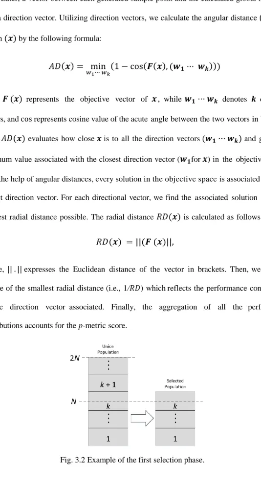
3.2 Example of the first selection phase ...30

3.3 Algorithm 1 ...32

3.4 Example of the second selection phase (case-I) ...34

3.5 Example of the second selection phase (case-II) ...35

3.6 Example of the second selection phase (case-

III) ...36

3.7 Algorithm 2 ...37

3.8 Algorithm 3 ...39

4.1 Non-dominated solution distributions for each algorithm on three-objective

DTLZ1, MaF1, MaF6 and MaF7 ...48

4.2 Non-dominated solution distributions for each algorithm on ten-objective

MaF1, MaF6, MaF8 and MaF13 ...49

4.3 5-D DTLZ1 ...50

4.4 10-D DTLZ1 ...50

4.5 5-D DTLZ2 ...51

4.6 10-D DTLZ2 ...52

4.7 5-D DTLZ3 ...52

4.8 10-D DTLZ3 ...53

4.9 5-D DTLZ4 ...54

4.10 10-D DTLZ4 ...54

4.11 5-D DTLZ5 ...55

4.12 10-D DTLZ5 ...55

4.13 5-D DTLZ6 ...56

4.14 10-D DTLZ6 ...56

CHAPTER I

INTRODUCTION

Optimization is extensively involved in many real-world problems. More often than not in physical world solving complex problems involves the simultaneous optimization of multiple conflicting objectives. Typically, these problems occur in various fields including engineering, chemistry, finance, physics and manufacturing. Some real-world scenarios include engineers aiming for the best performance of their designs; manufacturing representatives expect efficacy in their production systems; bank lenders try to minimize the risk of investment while maximizing the returns. Generally, the optimization process involves a number of design challenges in the form of optimizing some objectives and corresponding constraints. There exist many classical mathematical methods to solve multi-objective optimization problems. However, they at best offer adequate performance for a maximum of three objectives and fail to perform well in the environment of more than three conflicting objectives.

Most of the multi-objective evolutionary algorithms (MOEAs) utilize Pareto-dominance relationship, they perform quite well with three objectives, but, they were proven to be ineffective when the number of objectives is more than three. The reason for this scenario is that, most of the existing MOEAs utilize pair-wise comparison (i.e, tournament selection) and they lose their efficiency with more number of objectives. There by, dramatically increasing the number of non-dominated solutions with the increase in the number of objectives and to create some selection

pressure in this case is almost unattainable. Hence, MOEAs have very less to negligible success in tackling Many-objective optimization problems (MaOPs).

1.1 Problem Definition

MaOPs contain m (i.e., m>3) conflicting objectives to be solved concurrently. Generally, a MaOP can be defined by the following equation.

𝑓(𝑥) = (𝑓

1

(𝑥),··· 𝑓

𝑚

(𝑥))

(1)

s. t x ⊂ 𝜙

Here,

Φ ⊂ ℝ

_𝑛 is the search space,

𝑓: Φ → Ω ⊂ ℝ

_𝑚, and

Ω

is the objective space . Here

, 𝑚

are the number of decision variables and number of objectives respectively. For the sake of convenient discussions,

𝑓

₁

(𝑥)

is assumed as a minimization problem, where,

𝑓

₁

(𝑥),··· , 𝑓

_𝑚

(𝑥)

are a set of minimization problems. Usually, there is more than one solution for a specific minimization problem: multiple trade-off solutions also called Pareto-optimal solutions, which in turn forms a Pareto set (PS) in the decision space and is mapped as Pareto front (PF) in the objective space. So, an algorithm’s goal is to solve a minimization problem

(𝑓(𝑥)) t

o obtain a PF full of uniformly distributed solutions on it. To accomplish the same goal, numerous Multi-objective evolutionary algorithms were proposed in the last few decades.

Many researchers and practitioners are obliged to follow one between the two paths. The first path is to adjust the number of objectives they are dealing with to an algorithm or module which performs. Typically, this process is done by combining several objectives (can be conflicting) to one. This approach is not ideal because unlike treating objectives one at a time and optimizing them separately, optimizing a combination of objectives is bound to lose useful trade-off solutions. On top of it, combining two objectives without much knowledge of their objectives is very hard, if not impossible.

Generally, we think to develop strategies in order to reduce the number of objectives while retaining as much information of as many objectives as possible. For example, Brockhoff and Zitzler [1] initially identified conflict and nonconflictual relationships between each pair of objectives and then combined non-conflicting objectives into one objective. To find the correct lower dimensional interactions of each objective by iteratively starting from the interior of the search space heading for the Pareto-optimal region, Deb and Saxena [2] proposed a Principle Component Analysis method. Singh et al. [3] generated an approximate non-dominated front and came to conclusion whether an objective is redundant or not, just by having a look at the approximate front.

While objective reduction works in some special conditions, there are a lot of real-world problems whose objectives cannot be reduced any further. For those problems, the algorithms will only stick with the relatively important objectives [4]. Moreover, eliminating few objectives will not solve most of the MaOPs to produce desired results. Even after the number of objectives are reduced to a maximal extent, it is ambiguous as to how the derived Pareto front in a reduced low-dimensional space can mimic the true Pareto front in the original higher low-dimensional space. The second path is to make use of a number of algorithms, one for each dimension. This obviously is an inconvenient and a cumbersome approach, although it is just an alternative followed to avoid the problems caused in the first step.

In researchers’ perspective, the never-ending trade-off amongst convergence and diversity becomes much more complicated with the increase of the objectives. Moreover, the convergence and diversity dilemma are usually conflicting. Researchers’ often find it difficult to find the right balance between convergence and diversity as early emphasis on diversity will either delay the convergence or the solutions get stuck in a local optimum. Furthermore, relying on convergence alone will not produce all the trade-off solutions in most cases. Besides, it is almost inconceivable without a landscape of the solution set to adjudge which of the two (convergence and diversity) is the optimizer’s primary concern. On the grounds of that, most of the currently existing algorithms maintain relatively the same balance between the both. Without much ambiguity, one can say that

the final goal of this line of research is to design an algorithm that can dynamically adapt the delicate balance between convergence and diversity at any stage of the problem searching process.

1.2 Motivation

Solving the first problem involves careful construction an algorithm that can adapt the number of objectives at any stage of the problem scenario without any complicated mapping techniques. This step is usually important because every problem is categorized into either three or four-dimensional categories [5, 6, 7]. The actual range of the problem is further categorized into finer grains. Strictly speaking, categorized into one many-objective category does not mean that an eight objectives problem, for example, a 15-objectives problem should be treated in the same manner. In addition to that, the algorithms are usually inconsistent to either scale up (to solve dimensional problems higher than initially projected) or down (to solve dimensional problems lower than initially predicted), these inconsistencies makes it more difficult to rely on either one of them to develop the desired algorithm. Furthermore, to the algorithmic motivations, there are other practical motivations for the initial part of the study. We will discuss four of them here. First, in order to solve any optimization problem, it (the problem) must first be implemented (coded or expressed symbolically) within the optimizer (either a computer code or a commercial software). Often, this implementation process involves linking the optimizer to a third-party evaluation software such as a finite element or a computational fluid dynamics software or a network flow simulator etc. Secondly, in order to obtain better performance of the algorithm, customizing the optimizer itself for the problem at hand is recommended [8, 9] as it can be done either by introducing new operators or by modifying existing genetic operators utilizing the “heuristics”. For example, a heuristically biased initial population is preferred over generating a random initial population. These customized initializations and algorithmic modifications involve careful analysis, and are certainly time-consuming. Thirdly, we need to address each objective individually for most multi and

many-objective optimization methods in order to obtain ideal and Nadir points prior to solving the actual multi or many-objective version of the problem. Ideal points are obtained by individually optimizing each objective over the search space. Where, Nadir points are obtained from construction of worst objective function values of Pareto optimal solutions, it gets tougher when the objective functions increase. Often, we come across methods where, several lower-dimensional runs are implemented, executed to examine either the performance of the algorithm or to be certain in obtaining better high dimensional front [10]. Fourthly, in design exploration problems, objectives, constraints and decision variables are altered to get an even better idea of the possible range of optimal solutions [11]. Taking these four challenges into consideration, let us presume that a distinct optimizer is needed for each and every dimensional version of the actual optimization problem. In that case, for each and every optimizer the following changes has to be made: implementation of the problem, slight modifications in the algorithm and customized initializations. Thereby making the overall process slow, tiresome and prone to errors. Solving a single objective version of a multi-objective optimization problem will be so much more complicated as it requires a particular optimizer.

Finally, we need to design an optimizer which suits its dimensionality of every version of a design exploration problem, which in turn relies on the distinct combination of number of constraints decision variables and objectives. Alternatively, if an unified optimization algorithm competent of managing one-to-many objectives efficiently is available, modification of the algorithm based on heuristics, problem implementation and integrating with external evaluation soft-ware can only be done once which would be more convenient for solving different dimensional versions of the original problem. This provides flexibility for users to move back and forth amid different objective -dimensions of the same original problem and it saves a great deal of time, effort and most predominantly reduces if not free from process errors.

Developing a unified algorithm that can adapt to the dimension dynamically is only half the story. We also need to make sure that when it comes to more than one objective, the state-of-the-art algorithm should be able understand the scenario and emphasize on either convergence, diversity or both. Shifting the emphasis of the algorithm from one to another might help in discovering solutions that are difficult to attain otherwise and might as well reveal some interesting aspects about the optimization problem itself. It is very helpful for a practitioner with little or no knowledge about the problem to try and put emphasis only on convergence at one time and on diversity at another. This will give the direction to work with. After all, it is difficult to tell ahead of time, whether the problem need to emphasize on convergence or diversity. For the very reason it will be extremely helpful if the algorithm itself can solve the problem by dynamically adapting the need for more convergence or diversity.

Considering the above trends, we employ p-Metric based technique to design our MOEA in addition to non-dominated sorting. Combining both the methodologies gives a right balance between convergence and diversity for the MOEA. Later, we explain how we emphasize on either convergence or diversity at a specific stage by updating the direction vectors which addresses a tricky problem. By employing p-Metric based technique, we are equipped with p-Metric based visualization [91] tool. As mentioned before maintaining a right balance between convergence and diversity becomes next to impossible, with the increase in the number of objectives. This visualization tool helps the algorithm to monitor convergence performance and diversity performance at any stage of the algorithm, which makes our MOEA very accurate.

1.3 Thesis Statement

This thesis develops an APMOEA (Advanced p-Metric based Many-Objective Evolutionary Algorithm), where a two-phase selection scheme is employed which combines both non-dominated sorting and p-metric selection. Moreover, this thesis also proposes a modified p-metric

methodology in order to adjust the direction vectors dynamically. In the experiments, we compare APMOEA with four state-of-the-art Many-Objective EAs under, three performance indicators, including p-metric.

1.4 Thesis Organization

Chapter Two provides the literature review for each type of MOEAs for MaOPs. It presents the necessary background with references to each type of methods and analyzes pros and cons of them. It also lists widely used performance metrics and most popular benchmark functions and test suites for different scales of optimization tasks.

Chapter Three elaborates the proposed method of fitness evaluation based on p-metric. It also discloses a unique way to maintain the convergence and diversity by utilizing non-dominated sorting and both the fitness evaluations in the form of Radial Distance calculation (RD) and Angular Distance (AD). This chapter also provides algorithms and related framework of APMOEA and the two-phase selection strategy.

Chapter Four compares the performance of APMOEA with four other state-of-the-art Many-Objective EAs and we tabulate the results based on three performance metrics. The last one being the visualization based on p-metric method. We detail the experimental results for seventeen selected benchmark problems from both DTLZ, and MAF test suites. These problems offer various problem characteristics that present numerous degrees of complications for the underlying state-of-the-art Many-Objective EAs.

In Chapter Five, we concludes the study. We also provide recommendations for future work. Additionally, we probe on how one can extend APMOEA into a constrained many objective evolutionary algorithm.

CHAPTER II

LITERATURE REVIEWS

In this chapter, we review and analyze five classes of MOEAs in terms of their convergence and diversity methods used. For each class of MOEAs, we present an algorithm in detail to gain more insight.

2.1 MOEAs Based on Pareto-Dominance Modification

Firstly, there are a few designs which incorporate modified Pareto dominance concepts to adapt it to a higher dimensional space include Pareto α-Dominance [12], Pareto ε-Dominance [12], and Pareto cone ε-Dominance [12]. For all the above methods, parameters are heuristically integrated. Each modified Pareto dominance design is a relaxed form of the Pareto dominance in that it makes one individual dominates others easier in a high-dimensional space. Based on a similar idea, proposed a ε- Domination Based Multi-Objective Evolutionary Algorithm (ε-MOEA) [13] was proposed and has been performing well for MaOPs [14].

This class of MOEAs replace Pareto-dominance and provides a new fitness assignment measure to select individuals in the evolution process in order to push the whole population towards the true Pareto front. Accordingly, the convergence power mainly comes from the modified dominance relation, which is the domain criterion in the evolution process. Different modification methods can be considered as the adjustment of dominance degree, the degree level varies from one dominance relation to another. The hardest dominance level being the Pareto

Dominance where one individual is better than the other in one dimension if and only if its objective value is strictly smaller (for minimization problems) than the other. On the contrary, in ε -Dominance, one individual is better than the other in one dimension means that, it is not worse than the other in the same dimension, it might vary with some other dimension.

This design achieves diversity by using the parameter of degree, e.g., ε in ε-Dominance and α in α-Dominance. In addition to controlling the dominance degree, these parameters also determines the size of hyperboxes. Where in each of the hyperbox can contain no more than one individual in order to maintain the diversity.

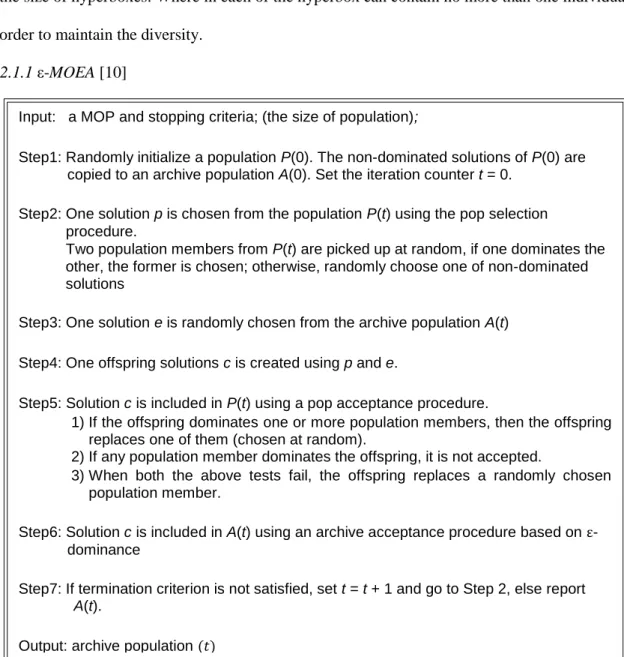
2.1.1 ε-MOEA [10]

Figure 2.1 General framework of 𝛆-MOEA Input: a MOP and stopping criteria; (the size of population);

Step1: Randomly initialize a population P(0). The non-dominated solutions of P(0) are copied to an archive population A(0). Set the iteration counter t = 0.

Step2: One solution p is chosen from the population P(t) using the pop selection procedure.

Two population members from P(t) are picked up at random, if one dominates the other, the former is chosen; otherwise, randomly choose one of non-dominated solutions

Step3: One solution e is randomly chosen from the archive population A(t) Step4: One offspring solutions c is created using p and e.

Step5: Solution c is included in P(t) using a pop acceptance procedure.

1) If the offspring dominates one or more population members, then the offspring replaces one of them (chosen at random).

2) If any population member dominates the offspring, it is not accepted.

3) When both the above tests fail, the offspring replaces a randomly chosen population member.

Step6: Solution c is included in A(t) using an archive acceptance procedure based on ε -dominance

Step7: If termination criterion is not satisfied, set t = t + 1 and go to Step 2, else report

A(t).

Based on the ε-dominance relation ε-MOEA is a steady-state algorithm. It breaks down the objective space into hyperboxes of size ε. Each hyperbox can contain at most a single solution on the basis of ε -dominance. From [13], ε -MOEA provides a tradeoff amongst convergence, diversity, and also computational time. Additionally, we can make it interactive with a decision-maker which refers that, ε can be chosen by a decision-decision-maker according to user’s preference.

ε-MOEA applies ε-dominance to direct the search towards the true Pareto front and ε-dominance plays a similar role like Pareto dominance in aiding the convergence of the population in low-dimensional space. Nonetheless, an improper choice of ε value will result in a poor performance of the algorithm. Furthermore, in the evolution process, ε-dominance can only be applied during the selection stage and still there is no help to handle the ineffectiveness of recombination operators caused by the large search space.

The diversity is kept by restricting each hyperbox with at most a single solution. Therefore, solutions are bound to have a minimum distance ε between them. By doing this we can only solve the distribution problem among solutions; as the spread of population cannot be improved. Moreover, a good distribution still requires a perfect ε value. If ε is way too small, solutions will be crowded with others. Whereas, a larger ε will eliminate more solutions in the beginning of the evolution process which is not ideal. Figure 2.1 shows the general framework of ε-MOEA.

2.2 Decomposition Based MOEAs

The second class is decomposition based designs, like Multiple Single Objective Pareto Sampling (MSOPS), and Multiobjective Evolutionary Algorithm based on Decomposition (MOEA/D) [15]. This type of designs decomposes a multi-objective optimization problem into a number of single optimization problems and predefines a group of search directions corresponding to these single optimization problems in order to optimize them concurrently. During the evolution process, Tchebycheff [15] and Achievement Scalarizing Function [5] can be applied as a fitness

assignment. The fitness values are used in selecting individuals instead of using Pareto-Dominance. For the very reason, this method can be adaptable to solve MaOPs.

In comparison with Pareto dominance, a group of weight vectors (search directions) are defined in advance and aggregate all objective values to push the population towards the true Pareto front; simultaneously, a solution can be recombined with another only if they are neighbors, which curtails a lot of difficulties from the large search space. However, the performance of algorithm is relies primarily on the selected aggregation method. When optimizing different problems, different aggregation methods must be chosen for each problem. For example, as stated in [28], weighted sum method is more efficient for convex problems while Tchebycheff method is advisable in nonconvex problems. Also, the number of weight vectors is equally important in respect to the performance. If this number of weight vectors is too small, each solution is very much different from solutions in its own neighborhood. As mentioned earlier, when recombining (crossover) two distant parents, chances of obtaining a good offspring are very low and the difficulty from large search space still exists. On the other hand, if the number of weight vectors is too large, it takes a lot of computational budget. In addition to that, in the high-dimensional search space, no one really knows in advance as to, how many weight vectors are sufficient for the evolution process, as we don’t know what a suitable population size is for a high-dimensional search space. Moreover, from a large search space if the neighborhood size is too large it will make so much harder for the algorithm to perform well.

The diversity of the population is maintained by a group of well distributed weight vectors or reference points. In the evolution process, each weight vector directs the respective individuals towards their reference point in the true Pareto front. However, well distributed weight vectors and sub problems cannot ensure that, their corresponding optimal solutions are well distributed too. In a high-dimensional search space, there could be one single solution, which is an optimal solution for multiple sub problems, which cause a severe damage to the population diversity [19].

Also, the size of the neighborhood still affects the diversity performance. This indicates that a smaller neighborhood size cannot ensure a good population diversity.

In summary, both convergence and diversity power are mainly dependent on well distributed weight vectors and the corresponding neighborhood. However, the difficulties of setting the number of weight vectors, neighborhood size, and the choice of aggregation method, make the algorithm harder to obtain good convergence or diversity performance.

Figure 2.2 General Framework of MOEA/D

2.3 Grid Based MOEAs

Input: An MOP and a stopping criterion;(the number of subproblems);

𝜆1_{, 𝜆}2_{, … , 𝜆}𝑁_{(a uniform spread of 𝑁 weight vectors); 𝑇(the number of weight vectors in} neighborhood of each weight vector)

Step1: Initialization 1) Set𝐸𝑃 = ∅.

2) Compute the Euclidean distances between any two weight vectors and then work out the 𝑇 closest weight vectors to each one. ∀ 𝑖 = 1, … , 𝑁 , set

(𝑖) = {𝑖1, … , 𝑖𝑇}, where 𝜆𝑖1_{, … , 𝜆}𝑖𝑇 _{are the 𝑇 closest weight vectors to 𝜆}𝑖 3) Generate an initial population 𝑥1_{, … , 𝑥}𝑁_{randomly. Set 𝐹𝑉}𝑖 _{= 𝐹(𝑥}𝑖₎ 4) 4) Initialize𝑧∗ _{= (𝑧𝑖∗, … , 𝑧𝑚∗ )}𝑇 _{by a problem-specific method.}

Step2: Update For 𝑖 = 1, …, 𝑁, do

1) Reproduction: Randomly select two indexes , 𝑙from 𝐵(𝑖) , and then generate a new solution 𝑦 from 𝑥𝑘 _{and 𝑥}𝑙 _{by using genetic operators.}

2) Improvement: Apply a problem-specific repair/improvement heuristic on 𝑦to produce 𝑦′

3) Update of 𝑧: for each 𝑗 = 1, … , 𝑚, if 𝑧𝑗 < 𝑓𝑖(𝑦′_{), then set 𝑧𝑗 = 𝑓𝑖(𝑦}′_{), .} 4) Update of Neighboring Solutions: for each index 𝑗 ∈ 𝐵(𝑖),if 𝑎𝑡𝑒_(𝑦′_𝜆𝑗_{, 𝑧) <} (𝑥𝑗_𝜆𝑗_{, 𝑧), set 𝑥}𝑗 _{= 𝑦}′ _{and 𝐹𝑉}𝑗 _{= (𝑦}′₎

5) Update of EP: Remove EP from all the vectors dominated by (𝑦′_{) and add (𝑦}′₎ to EP if no vectors in EP dominate 𝐹(𝑦′_).

Step3: Stopping Criteria

1) If stopping criteria is satisfied, then stop and output EP. Otherwise, go to Step2. Output: External Population (EP)

The third class is the grid-based method. In [16], a grid reflects the status of the convergence and diversity at the same time. Grid-Based Evolutionary Algorithm (GrEA) [16] focuses on the potential of the grid-based approach to increase the selection pressure towards the optimal direction, while maintaining exclusive uniformly distributed solutions. Territory Defining Multi-objective Evolutionary Algorithm (TDEA) [17] marks a territory around each individual to prevent the crowding problem. However, decision maker does not decide the hyperbox of TDEA; it is related to the individuals.

Grid based method employs grid coordinates in the process of evolution. This approach increases the selection pressure towards the global Pareto front simultaneously conserving an extensive and uniform distribution among solutions. As outlined in [16], when compared with Pareto dominance, a grid-based criterion can not only compare solutions qualitatively but also gives the quantitative comparison of objective values of the solutions. This characteristic provides main convergence power. However, the choice of the size of hyperbox and grid parameter can be a challenge. Meanwhile, the selection pressure towards the true Pareto front is hard to increase, as direct use of grid coordinates is not possible. On the contrary, it still requires aggregation methods or some fitness assignment techniques to handle these grid coordinates.

Like NSGA-III, Grid based method employs the idea of fitness sharing to maintain diversity. Here, based on its objective values population is divided into different boxes. In addition, we degrade each individual’s fitness if its hyperbox contains multiple individuals. Different methodologies implement different strategies; ε-MOEA minimizes one individual for each hyperbox, while GrEA only punishes individuals in the crowded hyperbox.

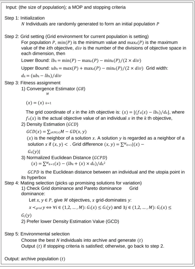
2.3.1 GrEA [16]

Figure 2.3 General Framework of GrEA Input: (the size of population); a MOP and stopping criteria Step 1: Initialization

𝑁 Individuals are randomly generated to form an initial population 𝑃 Step 2: Grid setting (Grid environment for current population is setting)

For population 𝑃, min(𝑃) is the minimum value and max𝑘(𝑃) is the maximum value of the 𝑘th objective, 𝑑𝑖𝑣 is the number of the divisions of objective space in each dimension, then

Lower Bound: 𝑙𝑏𝑘 = min(𝑃) − max𝑘(𝑃) − min𝑘(𝑃)⁄(2 × 𝑑𝑖𝑣)

Upper Bound: 𝑢𝑏𝑘 = m𝑎x(𝑃) + max𝑘(𝑃) − min𝑘(𝑃)⁄(2 × 𝑑𝑖𝑣) Grid width: 𝑑𝑘 = (𝑢𝑏𝑘 − 𝑙𝑏𝑘)⁄𝑑𝑖𝑣

Step 3: Fitness assignment

1) Convergence Estimator (𝐺𝑅)

𝑀 (𝑥) = (𝑥)𝑘=1

The grid coordinate of 𝑥 in the 𝑘th objective is: (𝑥) = ⌊(𝑓𝑘(𝑥) − 𝑙𝑏𝑘)⁄𝑑𝑘⌋, where 𝑓𝑘(𝑥) is the actual objective value of an individual 𝑥 in the 𝑘 th objective, 2) Density Estimation (𝐺𝐶𝐷)

𝐺𝐶𝐷(𝑥) = ∑𝑦∈𝑁(𝑥)𝑀 − 𝐺𝐷(𝑥, 𝑦)

(𝑥) is the neighbor of a solution 𝑥. A solution 𝑦 is regarded as a neighbor of a solution 𝑥 if (𝑥, 𝑦) < . Grid difference (𝑥, 𝑦) = ∑𝑀𝑘=1|(𝑥) −

𝐺𝑘(𝑦)|

3) Normalized Euclidean Distance (𝐺𝐶𝑃𝐷) (𝑥) = ∑𝑀𝑘=1(𝑥) − (𝑙𝑏𝑘 + (𝑥) × 𝑑𝑘)⁄𝑑𝑘2

𝐺𝐶𝑃𝐷 is the Euclidean distance between an individual and the utopia point in its hyperbox

Step 4: Mating selection (picks up promising solutions for variation) 1) Check Grid dominance and Pareto dominance Grid dominance:

Let 𝑥, 𝑦 ∈ 𝑃, give 𝑀 objectives, 𝑥 grid-dominates 𝑦:

𝑥 ≺𝑔𝑟𝑖𝑑 𝑦 ⟺∀𝑖 ∈ (1,2, … , 𝑀): 𝐺𝑖(𝑥) ≤ 𝐺𝑖(𝑦) and ∃𝑗 ∈ (1,2, … , 𝑀): 𝐺𝑗(𝑥) ≤ 𝐺𝑗(𝑦)

2) Prefer lower Density Estimation Value (GCD) Step 5: Environmental selection

Choose the best 𝑁 individuals into archive and generate (𝑡)

Output (𝑡) if stopping criteria is satisfied; otherwise, go back to step 2. Output: archive population (𝑡)

2.4 Performance Indicator Based MOEAs

The fourth class is based on the idea of developing the algorithms according to the quality indicators. These quality indicators aim at unfolding advantages and shortcomings of the state-of-the-art MOEAs and they determine the best performance associated to the specific problem characteristics by assigning a specific fitness measure for every individual. For instance, Volume Dominance (VD) [20] assigns fitness value which is equivalent to the volume dominated in the objective space by that particular individual. Contraction/Expansion of Dominated Area (CE) [21] regulates the selection process by altering the size of the respective individuals’ dominance area as well as the distance to the best known solution. Whereas, GB [22] evaluates the best reference point’s value that dominates the entire population size. Hypervolume Estimation Algorithm for Multiobjective Optimization (HypE) [23], is probably the most successful implementation of this class in that it has been shown to be more effective than other MOEAs for MaOPs. Also, there are a few other designs in a similar fashion like Indicator-Based Evolutionary Algorithm (IBEA) [24] and S Metric Selection Evolutionary Multiobjective Optimization Algorithm (SMS-EMOA) [25].

This type of designs implements any of the modified version of performance indicators to directly assign each individual a fitness value. The assigned fitness value should reflect both convergence and diversity performance of the individuals concurrently. In literature, these performance/quality indicators look at answering three main objectives [26]: minimizing the distance between the obtained non-dominated set to the true Pareto-Front, obtaining a uniformly distributed solution set in the objective space, and maximizing the obtained non-dominated front. Generally, all those indicators assign a value for the whole approximation front which reflect their performance. Here, these performance indicators are adjusted in such a way that, every individual of the approximate front is assigned a value based on its sole contribution to the overall

performance. Hence, the fitness value is directly proportional to the optimization, and instead of Pareto dominance it can be employed for selection of individuals and environmental mating (crossover/mutation) in the evolution process.

Nonetheless, many performance indicators alone cannot faithfully measure MOEA performance [27], the assigned fitness value by most of the indicators can only provide one perspective of the performance, but it is inconsistent in other perspectives of the performance. Which, results in using different quality indicators under some specific conditions. Furthermore, few indicators oppose Pareto-dominance by assigning the dominated individual a better score over the non-dominated one. Therefore, the selection of indicator is very important for the algorithm. Besides, even if the indicator is chosen soundly, this method only addresses a way for fitness assignment and it cannot limit the problems related to large search space.

2.4.1 HypE [15]

Figure 2.4 General Framework of HypE

Input: a MOP and stopping criteria; (the size of population); (reference set); Step1: Initialization

Initial population 𝑃 by selecting 𝑁 solutions uniformly at random Step2: Mating selection

1) Hypervolume-based fitness value Estimating b y Monte Carlo Simulation 2) Choose parents 𝑃′_{according to hypervolume-based fitness}

Step3: Variation

Generate offspring 𝑃′′_{from chosen parents 𝑃}′ Step4: Environmental selection

1) Combine 𝑃′′ _{and 𝑃 and select best 𝑁 individuals into archive population 𝐴(𝑡) based on} Pareto-dominance and hypervolume-based fitness values

2) Output 𝐴(𝑡) if stopping criteria is satisfied; otherwise, go back to step 2 Output: archive population (𝑡)

HypE is a hypervolume-based many-objective evolutionary optimization algorithm. It employs Monte Carlo simulation to evaluate the exact hypervolume value, and assigns ranks to the solutions induced by the hypervolume indicator. These ranks of the solutions are utilized in calculating fitness values, mating selection, and environmental selection. On a whole, it balances the accuracy of the estimates and the computational budget involved in the Hypervolume calculation. The modified hypervolume indicator can assign each individual a fitness value which reflects both convergence and diversity performance of that particular individual. Figure 2.4 shows the general framework of HypE.

2.5 Diversity-Emphasis Method

In this type of designs, diversity becomes the main criteria in the evolution process rather than convergence. Convergence is maintained by either the Pareto dominance or other methods which help in pushing the non-converged individuals into more crowded area [29].

When the Pareto domination resistance occurs in the higher dimensional space: all the individuals are non-dominated among each other, this sort of designs transforms the work directly from optimizing both convergence and diversity to improve only the diversity. So it is called the diversity-emphasis method.

2.5.1 NSGA-III [5]

NSGA-III is a hybrid algorithm, which has a framework similar to the original NSGA-II except it includes a refined diversity preservation technique especially for handling many-objective optimization problems instead of using crowding distance method. This technique works in this manner: at each generation, an ideal point is determined by finding the minimum value in each objective function among all current solutions; after that, objective values of the solutions are

rendered by deducting the original objective value from the ideal point. Later on, we identify the extreme solutions by Achievement Scalarizing Function (ASF); the identified extreme solutions and ideal point contain a hyper-plane. Next, many well-distributed reference points are generated on the hyper-plane prior to the evolution process. Every individual is associated with one of the reference points. Niche count of each reference point is evaluated, by determining the number of its respective population member associated. Finally, the population members associated with the reference point that has the smallest niche count value at the last accepted non-dominated front are selected.

Figure 2.5 General Framework of NSGA-III

Input: An MOP and a stopping criterion; (population size); (reference points)

Step1: Initialize population

A random parent population 𝑃0 is created. The population is sorted based on the fuzzy Pareto dominance. Each solution is assigned a rank equal to its Pareto domination level where 1 is the best level. Binary tournament selection, SBX recombination, and polynomial mutation operators are used to create a child population 𝑄0 of the same size 𝑁.Set 𝑡 = 0

Step2: 𝑅𝑡 = 𝑃𝑡 ∪ 𝑄𝑡

Combine parent and children population. The population 𝑅𝑡 will have size 2𝑁.

Step3: F=Non-nondominated-sort (𝑅𝑡) until |𝑃𝑡+1| < 𝑁.

Population 𝑅𝑡 is sorted based on the non-domination sorting. The new parent population 𝑃𝑡+1 is formed by adding solutions from the first front to the next best front (𝐹𝑙)before the size exceeds 𝑁.

Step4: Choose 𝑁 − |𝑃𝑡+1| solutions from 𝐹𝑙

1) Construct the hyperplane and normalize objectives of each solution 2) Associate each member with a reference point of 𝑍𝑟

3) Compute niche count of each reference point

4) Sort reference points in descending order with the number of associated population Members. Identify the first 𝑁 − |𝑃𝑡+1| reference points and choose their associated population members to construct new population

5) If stopping criterion is not satisfied, go back to Step2; otherwise, output 𝑃𝑡+1

Similar to NSGA-II, NSGA-III also applies Pareto dominance to sort the individuals and assign rank to every individual. Instead of relying on crowding distance at the final level, NSGA-III picks up the non-dominated point associated with the reference point with less niche count. This approach is efficient in maintaining diversity in the solutions and avoids the condition that happens with most of the aggregation methods: which means one single solution can be the optimal solution of many single objective optimization problems. In addition to that, this idea is very much like the concept of fitness sharing, which is a classic niching technique [30] and is used in punishing those solutions in the crowded area. That is, the population is sectioned into distinct groups of populations based on the similarity of the individuals in the population, in such a way that the population member is associated with the respective reference point in NSGA-III. Then, every individual’s fitness is decreased if more than one individual shares the same subpopulation with the reference point. Which means, in NSGA-III, individuals related to the reference point whose niche count is smaller have more chance to be chosen. Figure 2.5 shows the generic framework of NSGA-III.

2.6 Summary

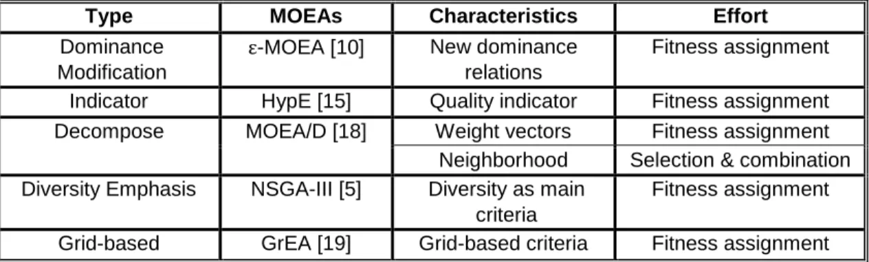
Usually, MOEAs have five major steps: population initialization, fitness evaluation, selection, recombination (crossover and mutation), and environmental selection. Recently proposed algorithms for solving MaOPs mainly focus on a modified technique for fitness assignment. For instance, ε-MOEA and algorithms of this type generally modifies the Pareto-dominance, HypE however, uses the hypervolume indicator, MOEA/D employs weight vectors, NSGA-III emphasizes on diversity performance, and GrEA incorporates a grid. Some of them also addresses few other aspects. For example, MOEA/D limits the selection, mutation and crossover to be done only in the neighborhood of the particular individuals. Meanwhile, NSGA-III choose large distribution index in recombination step. Table 2.1 is the summary of each type of MOEAs.

Table 2.1 Summary of Each Type of MOEAs

Type MOEAs Characteristics Effort

Dominance Modification

ε-MOEA [10] New dominance relations

Fitness assignment Indicator HypE [15] Quality indicator Fitness assignment Decompose MOEA/D [18] Weight vectors Fitness assignment

Neighborhood Selection & combination Diversity Emphasis NSGA-III [5] Diversity as main

criteria

Fitness assignment Grid-based GrEA [19] Grid-based criteria Fitness assignment

2.7 Performance Assessment

Researchers and Practitioners contributed to the Evolutionary Multi/Many-Objective Optimization literature in the design of performance criteria and methodologies for assessing performance of Evolutionary Multi/Many-Objective Optimization algorithms. It is necessary to select a relevant and effective method of performance assessment for either evaluating or comparing Evolutionary Multi/Many-Objective Optimizatx`ion algorithms. We use these methods of performance assessment to measure an algorithm's performance with respect to the convergence, diversity, and pertinence of the final approximation set. Most amongst the many methods of performance assessment rely on reference points or any equivalent to reference points. This dependency is not achievable in real-world problem scenarios, even more unlikely in the case where the problem is new and has not been subjected to optimization.

In this section, we explain three widely used performance metrics. Subsection 2.7.1 explains the Hypervolume Indicator metric, Subsection 2.7.2 outlines the Generational Distance metric, and Subsection 2.7.3 elaborates the Inverted Generational Distance metric.

2.7.1 The Hypervolume Indicator

The hypervolume indicator also known as “s-metric” is a performance metric introduced by [31] where it is described as the “size of the space covered or size of dominated space” for indicating the quality of a non-dominated approximation set,. Defined as below [32]:

𝑠

_𝑓𝑟𝑒𝑓

(x) = Ʌ(⋃

_x𝑛⊂x

[𝑓

₁

(x

_𝑛

), 𝑓

₁𝑟𝑒𝑓

] ×···× [𝑓

_𝑚

(x

_𝑛

), 𝑓

_𝑚𝑟𝑒𝑓

)

(1)

Here,

𝑠

_𝑓𝑟𝑒𝑓

(x)

resolves an issue associated with the size of the space covered by an approximation

set

x, 𝑠

_𝑓𝑟𝑒𝑓

(x) ⊂ ℝ

refers to a particular reference point chosen beforehand and Ʌ(. ) reflects the Lebesgue measure. This has been illustrated in Figure 2.6 in two-dimensional objective space (to allow for an easy visualization) with a population of 3 solutions.

Figure 2.6 an example of the hypervolume indicator in two-dimensional objective space

The hypervolume indicator is appealing because it is scaling independent and requires no prior knowledge of the true Pareto-optimal front. This is important when working with real-world problems which have not yet been solved. The hypervolume indicator is currently used in the field of multi-objective optimization as both a proximity and diversity performance metric, and in the decision making process as well [33, 34].

A vector of reference points is necessary to evaluate the hypervolume indicator value. When on comparison with a couple or multiple algorithms at the same time, reference vector employed must be the same; otherwise, the final hypervolume indicator values are not valid. In order to include the entire objective values in any approximation set to have a place in reference vector, we approximate the reference vector with all large values of each objective. A much better and accurate choice of a reference vector is to select the worst objective values from the union of approximation sets obtained on a particular test problem for different state-of-the-art evolutionary algorithms. Numerous versions of implementations of the use of hypervolume indicator have been presented in [35, 36, 37, 38, 39], all with the aim to aid its evaluation and computational time. The hypervolume indicator has been employed in the performance assessment of algorithms in much of the multi-objective optimization and evolutionary computation literature (e.g. [40, 41, 42, 43, 44]).

2.7.2 The Generational Distance

The Generational Distance (GD) introduced in [45, 46] measures the proximity of the approximation set to the true Pareto-optimal front in the objective space. We can express GD as given below:

𝐺𝐷 =

√∑𝑛∗_𝑖=1𝑑_𝑖2

𝑛∗ (2) where 𝑛∗ is the number of solutions in the approximation set, and 𝑑𝑖 represents the Euclidean distance (in objective space) amongst every solution in the approximation set to the nearest member on the true Pareto-Front. A zero GD value represents that every individual present in the approximation set are on the true Pareto-optimal front, and any value above zero illustrates the magnitude by which the approximation set is deviated from the true Pareto-optimal front. Calculation of GD is straightforward, at the same time the concept is very intuitive. However, prior knowledge concerning the true Pareto-optimal front is necessary for the reference vector. The

selection of solutions for the reference set will have an impact on the results obtained from the GD, and therefore the reference set must be diverse. In addition, the calculation of the GD can be computational expensive when working with a large populations or a high number of problem objectives. The GD measure has been widely employed to assess the performance of algorithms in most of the multi-objective optimization and in evolutionary computation literature (e.g. [47, 48, 49, 50, 51, 52]).

2.7.3 Inverted Generational Distance

Following with another performance metric, introduced an Inverted Generational Distance (IGD) which correct a known deficiency in the GD measure, measuring the proximity of the approximation set to the true Pareto-optimal front in the objective space. Below is the expression of IGD:

𝐼𝐺𝐷 =

√∑𝑛∗_𝑖=1𝑑_𝑖2

𝑛∗ (3)

Here, 𝑛∗ represents the number of solutions in the reference set, and 𝑑𝑖 represents the Euclidean distance (in objective space) amongst every solution in the approximation set to the nearest member on the true Pareto-Front. A zero IGD value represents that every individual present in the approximation set are on the true Pareto-optimal front, and any value above zero illustrates the magnitude by which the approximation set is deviated from the true Pareto-optimal front. This version of IGD implementation addresses an issue associated with its predecessor, which is that it will not rate an entire approximation set based on a single solution on the reference set as better than an approximation set which has more non-dominated (better) solutions that are much closer to the reference set. Yet, like the GD measure, prior knowledge concerning the true Pareto-optimal front is necessary in order to form a reference set. Moreover, solutions selected for the reference

set will have a huge impact on the results obtained from the IGD, and accordingly the reference set considered must be diverse. The IGD calculation can be computational expensive when working with either large reference sets or when high number of objectives are considered for the particular problem. The IGD measure has been exploited to assess the performance of the algorithms in most of the multi-objective optimization and evolutionary computation literature (e.g. [53, 54, 55, 56, 57]).

2.8 Benchmark Test Problems

In order to assess the performance of several nature inspired optimization algorithms, researchers and practitioners proposed numerous benchmark test problems. This section analyzes a few widely known and used benchmark test problems for large-scale optimization, multi- and many-objective optimization.

2.8.1 Benchmark Test Problems for Large-Scale Optimization

Tang et al proposed the first benchmark suite for large-scale optimization. in the CEC’2008 special session and competition on large-scale global optimization [62], known as the CEC’2008 suite, which consists of seven test problems. This is the first attempt where characteristics like separability and non-separability are explicitly included for large-scale optimization test problems. However, they roughly designed the problems to be either separable or non-separable; which is a major limitation of this test suite as this represents only two extreme cases of the most existing real-world problems.

On the verge of improving the CEC’2008 test suite, Tang et al. later proposed the CEC’2010 test suite [63]. The major advantage of CEC’2010 test suite over the previous one is that, CEC’2010 test suite employs modularity design principle, which in turn divides the decision variables into several subcomponents, and the separability of every subcomponent is independent to each another.

In the same way, with different combinations of separable and non-separable subcomponents, the test problems can be either fully partially separable, separable or fully non-separable. With the proposal of the CEC’2010 test suite, it has successfully motivated the development of techniques such as random grouping [64], cooperative co-evolution [60], and differential grouping [65]. As a further improved version of the CEC’2010 test suite, they included some new characteristics [66] and proposed the CEC’2013 test suite. Firstly, the subcomponents of the decision variables in the CEC’2010 test suite are completely independent, while in the CEC’2013 test suite, some subcomponents are overlapped. Secondly, all the subcomponents in the CEC’2010 test suite have a fixed size, while in the CEC’2013 test suite; the subcomponents are of different sizes, such that they have non-uniform contributions to the objective function.

2.8.2 Benchmark Test Problems for Multi- and Many-objective Optimization

Many researchers designed test suites for empirical studies to evaluate the performance of various MOEAs. Among many others test suites, the ZDT test suite [67], DTLZ test suite [68,69] and the WFG test suite [70, 71] are the most widely known and used ones. The ZDT test suite is one of the most popular if not the most popular test suites in the multi-objective optimization literature [67]. Deb based on the generic design principles in [72], proposed the test problems in the ZDT suite. By introducing three basic functions, including a distribution function f1, a distance function g and a shape function h are constructed. Where function f1 represents the ability to test an MOEA to maintain the diversity along the PF. While, function g is meant for testing the ability of an MOEA to converge to the PF and function h for defining the shape of the PF. On a whole, ZDT test suite consists of six test problems, five of them (ZDT1 to ZDT4, ZDT6) are real-coded and one (ZDT5) is binary-coded. Characteristics of ZDT test problems differ from one problem to another. Typically, ZDT3 has a disconnected Pareto-Front: which is partially convex and partially concave; ZDT4 consists of a large number of local PFs; ZDT6 has a fitness landscape, which is non-uniform in nature, which eventually cause a biased distribution of the Pareto optimal solutions along the PF.

Although, the ZDT test suite has gained immense popularity over the years, it still has a significant limitation, i.e., all test problems are bi-objective (two objectives).

To overcome the shortcomings of the ZDT test suite (as well as many other bi-objective test problems), Deb et al. proposed a new test suite, i.e., the DTLZ test suite [68, 69], which contains test problems which are scalable to any desired number of objectives. DTLZ test suite contains nine test problems; in constructing every one of them, utilized design principle is the same. Where, the first (M −1) decision variables describe the Pareto Optimal Front, while the remaining decision variables define the convergence property. The DTLZ test suite also have many exclusive characteristics. For example, the majority of the fitness landscape of DTLZ1 and DTLZ3 consists of a large number of local PFs; the distribution of the Pareto optimal solutions of DTLZ4 is usually non-uniform; the Pareto-Fronts of both DTLZ5 and DTLZ6 are a degenerate curve; DTLZ7 has a broken (not continuous) Pareto-Front; and DTLZ8 and DTLZ9 are constrained problems. A significant contribution of the DTLZ test suite would be the proposal of a generic design principle for constructing test problems that are scalable to have any number of objectives, as well as decision variables.

Many researchers have developed additional alternatives of the DTLZ test suite. To assess the performance of MOEAs on highly scaled problems [61], Deb et al. proposed a method to scale the value of each objective function to a different range. [73] suggests, some constrained DTLZ problems to verify the MOEAs constraints handling capacity. Nonetheless, the fact that DTLZ test suite is extensively used in the computational intelligence community it still has a few drawbacks. For instance, DTLZ test suite does not take some important characteristics commonly seen in the real-world problems into account, such as variable linkage and variable separability. In this context, separability means the correlation relationship amongst the decision variables in the entire decision space, while to characterize the relationship between the decision variables of Pareto optimal solutions they use variable linkage.

To avoid the deficiencies of the DTLZ test suite, Huband et al. proposed a whole new test suite, i.e., the WFG test suite [70, 71]. The WFG test suite employs an array of important characteristics that generally exist in real-world problems. In order to design a test problem, it only requires specification of a shape function, which in turn finds the PF, and a transformation function, which determines the fitness landscape. In the WFG test suite, test problems WFG1, WFG7 and WFG9 have partial PFs; WFG5 and WFG9 have misleading fitness landscapes; WFG2, WFG3, WFG6, WFG8 and WFG9 have fitness landscapes, which are non-separable. Since these test problems are also compatible with scalability concerning number of objectives, the WFG test suite becomes another extensive benchmark for many-objective optimization, apart from the DTLZ test suite. In addition to the above three general-purpose test suites, Researchers constructed other test problems to include some specific characteristics. In [74], Okabe et al. proposed quite a few design principles to construct test problems with an arbitrarily complex Pareto-Set, generalized from [58]. In recent years, Saxena et al. have extended the same test problems with complicated Pareto-Sets for many-objective optimization problems [75]. Few other modification versions of ZDT and DTLZ test problems can be found in [59] [76], where linear or nonlinear variables are introduced into decision variables. Although, the test problems detailed above are static, some Researchers proposed dynamic multi-objective optimization test problems in [77], where the PFs and/or PSs keep changing with respect to time. In [78, 79] some variants of these test problems can also be found.

CHAPTER III

PROPOSED ADVANCED p-METRIC BASED MANY-OBJECTIVE EVOLUTIONARY ALGORITHM

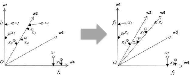
In this section, we propose an advanced p-metric based Many-Objective EA (APMOEA) for tackling both MOPs as well as MaOPs. We employed a two-phase selection strategy, which unites both non-dominated sorting and p-metric as well. During the first phase, we use non-dominated sorting to remove solutions with poor convergence. Despite the fact that non-dominated sorting often fails in many-objective cases, it can help eliminate the far-off individuals and assure the stability of the convergence. In the second phase, p-metric comes into picture to find the final set of reserved solutions, while we also proposed a modified method to maintain a proper set of the direction vectors of p-metric. We summarize the contributions as follows:

1) On comparison with a few other indicator-based EAs, APMOEA does not include additional parameters. In addition to that, due to the aggregate effect of non-dominated sorting and p-metric, APMOEA is very efficient in tackling both MOPs and MaOPs. 2) In APMOEA, we propose a modified performance-contribution evaluation method of p

-metric, in order to assist the enhancement of the diversity maintenance. That very adjustment makes p-metric possible to adapt to the situations for evolving the population.

3) During the evolution process, in the p-metric based selection the direction vectors set keeps changing with respect to time, in accordance with the current population distribution in

the objective space.

4) In the experiment setup, we test on seventeen problems, among three-, five- and ten-objective cases, with respect to the three performance indicators. Four of the problems included are regular test problems and are widely-used, while the rest of the 13 problems, specifically designed for the CEC 2017 competition, have either irregular, degenerate, disconnected, badly-scaled, mixed, (or) many other complex PFs. On comparison with four other most widely-used state-of-the-art Many-Objective EAs, the empirical results identifies that APMOEA has promising adaptability in tackling both MOPs and MaOPs with different types of PFs.

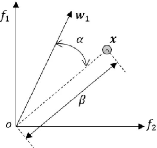
Fig. 3.1 Example of the angular and radial distances.

3.1 p-metric Measurement Method

In 2016, He and Yen proposed Polar-Metric (p-metric) to measure the performances of the state-of-the art multi-objective and many-objective EAs. A preset set of direction vectors in the objective space plays a major role in the p-metric measurement. First, we uniformly sample a set of points on the PF and then we calculate a global ideal point by getting the minimum value of each objective

vector. Later, a vector between each generated sample point and the calculated global ideal point forms a direction vector. Utilizing direction vectors, we calculate the angular distance

(𝐴𝐷)

of a solution

(𝒙)

by the following formula:

𝐴𝐷(𝒙) = min

𝑤1··· 𝑤𝑘

(1 − cos(𝑭(𝒙), (𝒘

𝟏

··· 𝒘

𝒌

)))

(1)

Here,

𝑭 (𝒙)

represents the objective vector of

𝒙

, while

𝒘

_𝟏

··· 𝒘

_𝒌 denotes 𝒌 direction vectors, and cos represents cosine value of the acute angle between the two vectors in brackets. Then,

𝐴𝐷(𝒙)

evaluates how close

𝒙

is to all the direction vectors (

𝒘

_𝟏

··· 𝒘

_𝒌

)

and gives the

minimum value associated with the closest direction vector (

𝒘

_𝟏for

𝒙

) in the objective space. With the help of angular distances, every solution in the objective space is associated with the closest direction vector. For each directional vector, we find the associated solution with the smallest radial distance possible. The radial distance

𝑅𝐷(𝒙)

is calculated as follows:

𝑅𝐷(𝒙) = ||(𝑭 (𝒙)||,

(2)

Where, || . || expresses the Euclidean distance of the vector in brackets. Then, we find the inverse of the smallest radial distance (i.e., 1/𝑅𝐷) which reflects the performance contribution of the direction vector associated. Finally, the aggregation of all the performance contributions accounts for the p-metric score.

Fig. 3.1 explains both the angular distance and radial distance in a bi-objective space, where 𝒘𝟏 being a direction vector and x is one of the solution. According to (1) and (2), an acute angle α represents the angular distance between 𝒘𝟏 and 𝒙 in Fig 3.1, while the radial distance of 𝒙 is equal to the distance β. In actuality, there are three different types of radial distance calculations employed in p-metric, corresponding to three different Pareto-Front shapes. However, when we apply p-metric to evolution, learning the shape of the PF beforehand is highly unlikely. Therefore, we only employ Euclidean distance type of radial distance measurement, universally used for the proposed algorithm.

3.2 Proposed Algorithm: APMOEA

In this section, we first emphasize two of the selection phases, the first selection phase based on non-dominated sorting and the second selection phase based on p-metric, respectively. Then, we outline the general framework of APMOEA.

3.2.1 First Selection Phase

In the first selection phase, the idea of using non-dominated sorting is to remove the remote solutions, in order to enhance the convergence stability. [82] Explains that we can sort a population into a series of dominated fronts, while solutions in the same front are non-dominated to each other and those in the lower-rank front dominate solutions in the higher-rank front. Assume that there exists 2N solutions in the population, and N solutions are all we need for the next generation, shown is an example for selecting N solutions in Fig. 3.2.

In Fig. 2, we sort a total of 2N solutions into several non- dominated fronts, while the front number and front rank exhibits an inversely proportional relationship, (i.e., the greater the front number, the lower is the rank). To reserve a minimum of N solutions, we choose the first k fronts. The number of solutions present within k fronts should range between N and 2N. Typically, while

tackling MaOPs, it is highly likely that all the solutions are stuck in one non-dominated front, making the first selection phase less effective. Nonetheless, for tackling MOPs the first selection phase is still valid, and can assist in getting rid of remote points to some degree.

3.2.2 Second Selection Phase

In the second selection phase, we use a set of uniformly distributed direction vectors, preset by the Das and Dennis’s method [50], to select the final reserved solutions.

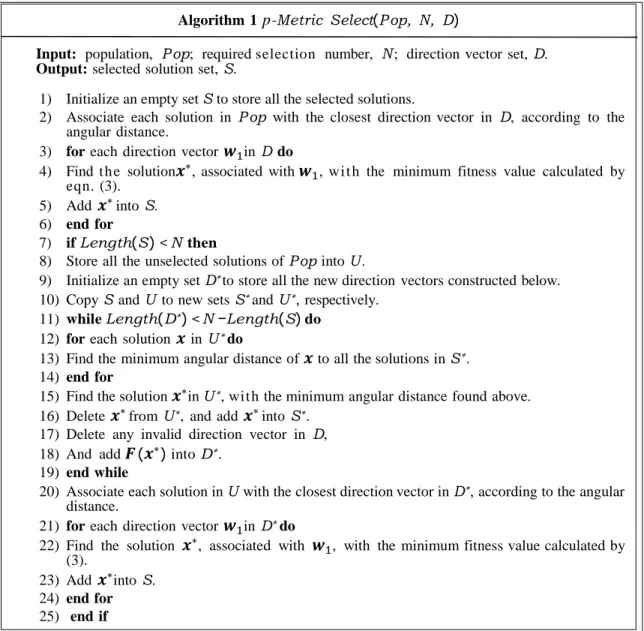
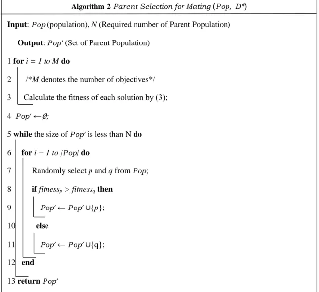
Fig 3.3 Algorithm 1

Algorithm 1 p-Metric Select(P op, N, D)

Input: population, P op; required selection number, N ; direction vector set, D. Output: selected solution set, S.

1) Initialize an empty set S to store all the selected solutions.

2) Associate each solution in P op with the closest direction vector in D, according to the angular distance.

3) for each direction vector 𝒘₁in D do

4) Find t he solution𝒙∗, associated with 𝒘1, wi t h the minimum fitness value calculated by eqn. (3).

5) Add 𝒙∗into S.

6) end for

7) if Length(S) < N then

8) Store all the unselected solutions of P op into U .

9) Initialize an empty set D∗to store all the new direction vectors constructed below. 10) Copy S and U to new sets S∗and U ∗, respectively.