Al-Khafajiy, M, Baker, T, Al-Libawy, H, Maamar, Z, Aloqaily, M and Jararweh, Y
Improving Fog Computing Performance via Fog-2-Fog Collaboration
http://researchonline.ljmu.ac.uk/id/eprint/10644/
Article
LJMU has developed LJMU Research Online for users to access the research output of the University more effectively. Copyright © and Moral Rights for the papers on this site are retained by the individual authors and/or other copyright owners. Users may download and/or print one copy of any article(s) in LJMU Research Online to facilitate their private study or for non-commercial research. You may not engage in further distribution of the material or use it for any profit-making activities or any commercial gain.
The version presented here may differ from the published version or from the version of the record. Please see the repository URL above for details on accessing the published version and note that access may require a subscription.
For more information please contact [email protected]
Citation
(please note it is advisable to refer to the publisher’s version if you
intend to cite from this work)
Al-Khafajiy, M, Baker, T, Al-Libawy, H, Maamar, Z, Aloqaily, M and Jararweh,
Y (2019) Improving Fog Computing Performance via Fog-2-Fog
Collaboration. Future Generation Computer Systems, 100. pp. 266-280. ISSN
0167-739X
Improving Fog Computing Performance via
F
og-2-
F
og Collaboration
Mohammed Al-khafajiya, Thar Bakera, Hilal Al-Libawyb, Zakaria Maamarc, Moayad Aloqailyd, Yaser Jararwehe
aDepartment of Computer Science, Liverpool John Moores University, Liverpool, UK bDepartment of Electrical Engineering, University of Babylon, Babylon, Iraq
cCollege of Technological Innovation, Zayed University, Dubai, UAE dGnowit Inc., Ottawa, ON, Canada
eJordan University of Science and Technology, Irbid, Jordan
Abstract
In the Internet of Things (IoT) era, a large volume of data is continuously emitted from a plethora of connected devices. The current network paradigm, which relies on centralized data centers (akaCloud computing), has become inefficient to respond to IoT latency concern. To address this concern, fog computing allows data processing and storage “close” to IoT devices. However, fog is still not efficient due to spatial and temporal distribution of these devices, which leads to fog nodes’ unbalanced loads. This paper proposes a newFog-2-Fog (F2F) collaboration model that promotes offloading incoming requests among fog nodes, according to their load and processing capabilities, via a novel load balancing known as Fog Resource manAgeMEnt Scheme (FRAMES). A formal mathematical model ofF2Fand FRAMES has been fomulated, and a set of experiments has been carried out demonstrating the technical doability ofF2F collaboration. The performance of the proposed fog load balancing model is compared to other load balancing models.
Keywords: Internet-of-Things, Fog computing,Fog-2-Fog collaboration, Offloading
1. Introduction
In the last few years, major advances in Information and Communication Technologies (ICT) have been witnessed. Such advances are anchored to different paradigms such as Information Centric Net-work (ICN) (e.g., mainframe), Software Defined NetNet-work (SDN), and Data Center NetNet-work (DCN). ICN shifted inter-networking to a cloud-based computing model, as reported in Cisco Cloud
In-5
dex (2013-2018) [1]. Since most Internet traffic originates and/or terminates to/from the cloud [1] [2], it is predicted that nearly two-thirds of total workloads obtained from traditional IT services (e.g., data aggregation and processing) will be processed on the cloud [1] [3]. Cloud computing enables users to access a variety of configurable facilities such as data storage, processing, infrastructure, and applica-tions [4], providing Everything-as-a-Service (*aaS) in return of a fee. Embracing the clouds, Internet
10
service providers and corporate IT service providers have become more motivated to adopt cloud com-puting; they can obtain a wide range of services with minimal administration [4] [5]. The inclination to use the clouds coincides with the improvement of Network Function Virtualisation (NFV) tech-nique which reduces cloud CAPital EXPenditures (CAPEX) and OPerating EXpenditures (OPEX), and improving the flexibility and scalability of an entire network [6]. Similarly, NFV has been used to
15
address the problem of deploying replica servers in clouds by proposing an algorithm based on spectral
∗Corresponding author: Thar Baker
Email addresses: [email protected](Mohammed Al-khafajiy),[email protected](Thar Baker),
[email protected](Hilal Al-Libawy),[email protected](Zakaria Maamar),
clustering theory [7]. The performance of the proposed solution on large-scale setup has shown lower deployment costs and improved data fusion.
Within the emerging Internet of Things (IoT), a large number of “smart” devices and objects (e.g., wearable) are, nowadays, connected to the Internet [8], generating high volumes of data every
20
second. In the IoT area, the word“thing”could be anything refers to everything that can connects to a network and exchanges data over this network [9] with other stakeholders (e.g., users, applications, and peers). Cisco IBSG estimates that approximately 50 billion devices (i.e., things) will be connected to IoT networks by 2022 [10] [11]. Although cloud can provision efficient data storage and processing facilities, the ever-growing volume of data will result in a high energy consumption, heavy burden on
25
the communication bandwidth [1] [12], and ”unacceptable” latency [13] [4] [14]. In addition, since the cloud is relatively “far” from IoT devices, by the time the data reaches the cloud for storage and/or processing, its importance and freshness could deprecate [15] [16]. To address cloud limitations with focus on latency in IoT, Cisco has come up with the concept of Fog in 2014 [1]. Security of mobile edge and fog is one of the major challenges for successful implementation and deployment of IoT
30
infrastructure. For example, researchers in [17] [18] [19] explore how to protect critical system (i.e., fog and edge) from unauthenticated or malicious attacks. However, the security aspect is part of our future work and has not been considered in the current work.
Simply put, fog is described as a highly virtualised platform that provides similar cloud facilities in terms of storage, processing, and communications at the edge of the network, “closer” to things
35
compared to cloud; i.e., between things and clouds [20], making these facilities fast, secure, and reli-able [21] [15]. Fog is not a substitute to cloud but a complement [1] since both are expected to work together [2] [22]. In general, thef og can support, serve, and facilitate services that are not appropri-ately served by cloud such as, (i) latency-sensitive services (e.g., healthcare and online gaming) [13]; (ii) geo-distributed services (e.g., pipeline monitoring) [23]; (iii) mobile services with high speed
con-40
nectivity (e.g., connected vehicles) [24]; and (iv) large scale distributed control systems (e.g., smart energy distribution and smart traffic lights) [1]. Despite the appealing benefits of fog computing, some concerns are undermining its adoption. This includes how to specify Cloud-2-Fog (C2F) collabora-tion andFog-2-Fog (F2F) collaboration. This paper addressesF2F by promoting service offloading among fog nodes so, that, minimal latency for IoT services is achieved.
45
1.1. Problem Statement
Althoughf og nodes are placed “closer” to IoT things so, that, latency is “taken care” of [13] [25], these nodes can quickly become congested when the number of requests soliciting their services exceed their capabilities [13] [24]. OpenFog [26] reports that, although fog computing provides extensive peer-to-peer interconnection for communication purposes with the clouds, its nodes run in silos, where no
50
collaboration capability, for job processing, is available. Therefore, fog resource management is needed to unlock the silos and free them from the historical stovepipes working pattern. In fact, poor resource management can cause latency and inefficiency for services within the fog [27] [28].
1.2. Research Contributions Our contribution is threefold:
55
1. F2F collaboration model that achieves a near optimal workload among the collaborating fog nodes (Section 3.1).
2. A Fog Resource manAgeMEnt Scheme (FRAMES) that promotes load balancing to address the latency concern of service request’s received from things. We adopt the notion of fog-as-a-service [29] where each fog node hosts local computation, networking and storage
capabili-60
ties. (Section 3.2).
3. A formal mathematical model that backs the decision of load balancing among fog nodes (Sec-tion 4).
1.3. Paper Organization
The remainder of this paper is organized as follows. Section 2 discusses the related work of fog
65
computing and services offloading. Section 3, describes the system architecture and management of fog nodes alongside our offloading approach in detail. Section 4 presents system design and modelling. Extensive simulation results and evaluations are presented in Section 5. Section 6 concludes the paper and discusses future work.
2. Related Work
70
Current research efforts into fog tackle the following challenges:
• Heterogeneity: fog nodes are diverse in terms of processing, storage and communication capabil-ities.
• Elasticity: the ever-growing number of IoT devices would trigger fog elastic.
• Federation: despite fog elasticity, making fogs collaborate is an option, when this elasticity
be-75
comes insufficient. However, heterogeneity is an obstacle to their collaboration.
Agarwal et al. [30] focus on resource allocation in a fog context. They propose a 3-layer architecture, client, fog, and cloud, that allows to distribute the workload between the cloud and fog nodes. In fact, the authors check whether enough processing is available on the fog node so, that, all or some tasks are executed or even postponed. Tasks could also be directed to cloud nodes. Agarwal et al.’s work
80
tackles well the heterogeneity challenge but neither scalability nor federation challenge are tackled. Beate et al. [31] propose a job placement and migration approach for providers of infrastructure that incorporate cloud and fog. The approach ensures end-to-end latency restrictions and reduces network usage by planning load migration ahead of time. The authors also discuss how the application knowledge of Complex Event Processing (CEP) can reduce the required bandwidth of Virtual Machines
85
(VMs) during their migration. However, the presented work does not consider offloading load among fogs; fogs are assumed able to perform computationally intensive tasks, which might not always be the case. In addition, with regard to the above challenges, the authors indicate that the approach can be employed at large scale in real world so, that, scalability is met. However, they seem overlooking heterogeneity and federation. Vehicular ad-hoc networks (VANET) have reached the maturity stage in
90
term of communication reliability with the benefits of information transmission between vehicles and surrounding fog and edge nodes [32] [33]. The quality of communication between vehicles and those nodes is being investigated. Many researchers have found that physical factors can impact this QoS especially in the presence of buildings and other obstacles (i.e., signal fading). A candidate solution is to utilize parked vehicles for routing communication [34].
95
A collaborative resource sharing and utilization among fog/edge was introduced recently with very promising solution employing 5g and composition techniques [35] [36]. Abedin et al. [35] propose resource sharing among fog nodes by defining a utility metric for these nodes that accounts the com-munication benefits in case resources are shared among them. First, the authors determine an organised list of preferences that paires fog nodes for each node. Then, each node in the fog places a request
100
of pairing with its preferred pairing nodes. At the reception side, depending on the preference and benefits of the previously received requests, a target node decides either to accept or to reject the request. The limitation of this work is that the pairing decisions are made based on communication cost without considering time and location. The authors do not also take the Quality-of-Service (QoS) (such as latency and bandwidth) in consideration as part of the resource sharing decision. Abedin et
105
al. considers the heterogeneity of nodes, as the resource limitation of fog nodes (e.g., CPU) has been considered during load allocation. However, the evaluation is conducted over a small scale making the scalability limited and hence, not met. In addition, federation is not relevant for this context, since the developed algorithm targets a single fog domain.
Lina et al. [37] propose a fog computing based resource allocation policy using Priced Timed
Petri-110
Nets (PTPNs). A simulation was developed to evaluate the proposed resource allocation strategy using parallel machines and Linux cluster. The outcomes were that the proposed resource allocation policy can provide efficient resource selection for autonomous task scheduling and improve the use of fog resources. The limitation of this work is the small-scale context related to online shopping, and the process of resource allocation is not automated calling for user assistance. While the authors meet
115
federation, scalability and heterogeneity are not met.
Sun et al. [38] propose Cloud-of-Things and Edge Computing (CoTEC) scheme for traffic man-agement in multi-domain networks. CoTEC direct the traffic flow through service nodes. The authors assign a critical egress point for each traffic flow in the CoTEC network using multiple egress routers to optimize the traffic flow; this is known as Egress-Topology (ET). Therefore, the proposed ET
incorpo-120
rates traditional multi-topology routing in the CoTEC network to address the inconsistencies between service overlay routing and border gateway protocol policies. Furthermore, Sun et al. introduce several programmable nodes that can be configured to ease the ongoing traffic on the network and realign services among other nodes in multi-domain networks. In regard to the above challenges, the federation is only met with edge-cloud, however the congestion of clouds or edges not discussed. Also, they seem
125
overlooking heterogeneity (i.e., device’s capacity) and scalability.
Despite all efforts mentioned beforehand, and to the best of our knowledge, a systematic framework forF2F collaboration that tackles heterogeneity, elasticity, and federation is still absent. This paper serves as a starting point for defining such a collaboration model.
3. Fog-2-Fog Collaboration Model
130
Before we dive into the proposedF2F collaboration model, we highlight the adapted fog comput-ing architecture. This architecture is similar to other large-scale computcomput-ing architectures (e.g., cloud computing) have either application specific architecture or application agnostic architecture. However, there is no a standard architecture for the systems that use fog computing [1] [12] [39]. In this pa-per, we adopt a general fog computing architecture that is in-line with the architectures presented
135
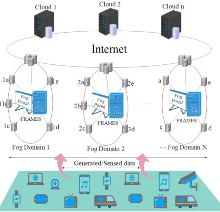
in [1] [2] [4] [12] [13]. Understanding the fog computing architecture topology helps obtain a bet-ter insight into the main functionality and benefits of using fog computing. The main layers in fog architecture arething,f og, andcloud(Figure 1).
Thing layer: also called perception layer, ensures data availability by hosting networked
de-vices (e.g., heart-rate and blood-oxygen sensors). Each device has a communication protocol (such
140
as IEEE 802.15.4, WiFi, Bluetooth, MQTT, etc.) so, that, it transmits the generated data to the fog layer in the form of data processing service request.
Fog layer: contains a number of distributed fog nodes that should ideally be located “next” to
data sources. This layer refines and processes the data that the things layer submits. Fog has the potential to reduce the amount of things’ data transmitted to the cloud layer by acting on these data.
145
Each fog node is equipped with onboard computational resources, data storage, alongside network communication facilities to bridge things and cloud within the IoT network [13].
Cloud layer:enables omnipresent, convenient, and proper network access to shared resources (e.g., stor-age and services processing) over the IoT network.
150
In the following, we define an IoT network as{T, F, C, L}, where:
• T is a set of things {t1, t2, .., tn}; tn is a 3-tuple format hn, ty, di where n is a thing
identi-fier (e.g., IP address),tyis a thing’s type according to the packet’s payload size1generated from
the thing (e.g.,heavy-packet andlight-packet), andd denotes the destination fromtn to the
1A payload size of 1024 Bytes can be transported without any fragmentation through a normal not constrained
Figure 1: IoT fog architecture composed ofthings,f og, andcloudlayers
nearest fog node (i.e., the first fog node that receives a service request from tn) within the fog
155
layer, and this is subject to change according totn’s location.
• F is a set of fog nodes{f1, f2, .., fi};fi is a 4-tuple formathi, `, s,}, riwhereiis a fog identifier
(e.g., IP address),` denotes a fog node location,s and }refer to services (e.g., image
process-ing) provided by the fog node and hardware capability (i.e., CPU frequency) of the fog node, respectively, andr is a set of all “reachable fogs”2 fromf
i.
160
• C is a set of cloud nodes, each c is defined using a 3-tuple format hi, `, siwhere i is the cloud identifier, ` denotes the cloud location, and s denotes the cloud services (e.g., processing and storage).
• L is set of communication links among the layers, such that,
L⊆ {hn,n, q` i|(n,n`)∈(T, T)(T, F)(F, F)(T, C)(F, C)(C, C)(C, F)(F, T)(C, T)V
(q∈Q)}.
165
This means,L is a sub-/set of available links betweenT hing←→F og←→Cloud. Each link is associated with itsqfromQset, which refers to the QoS properties (e.g., uploadb↑and download
b↓ bandwidth).
The standardised approach in which IoT systems (with a fog layer) operate is as follow:tngenerates
and gathers data periodically from the surroundings and sends it to either the fog layer or the cloud
170
layer for processing/manipulation. In the fog layer,fi can servetn’s request instantly or offload it to
another fog node (e.g.,fj) in the same domain iffiis congested and may delay processingtn’s request.
To this end,fi (orfj) responds back totn and reports to cloudci for data archiving. Similarly, when
packets are sent toci, it will be processed at this level and a response goes back totn. It is worth noting
that the importance of fog layer location (i.e., in-between thing and cloud layers), makes fogs more
175
accessible/reachable for both things and clouds. Therefore, fog can be used horizontally (i.e.,F og-2-Fog) and vertically (i.e., T hing←→ F og ←→ cloud) in the network to provide the desired services with high QoS. However, this paper’s focus is only on processing service’s requests dispatched from the things layer to fog layer in which the latter layer adopts the proposedF2F collaboration for efficient
data processing. The following sub-sections present the fog load balance by answering when and where
180
to offload a request, and then, discuss the fog resource management scheme. 3.1. Fog load balancing
Considering a scenario where a fog node accepts a data processing request from a thing; it will process the request and respond back. However, when the fog node is busy processing other requests, it may only be able to process part of the payload and offload the remaining parts to other fog nodes.
185
There are two approaches to model interactions among fog nodes. First, the centralised model, which relies on a central node that controls the offload interaction among the fog nodes. Second, in which each fog node runs a protocol to distribute their updated state information to the neighbouring nodes. Then, each fog node holds a dynamically updated list of best nodes that can serve the offloaded tasks. We envisage that the distributed model is more suitable for scenarios where things are mobile objects
190
(i.e., Internet of moving things [41]) as to support the mobility and flexibility of data acquisition. Therefore, we adopt this model of interactions in ourF2F collaboration model.
3.1.1. When to offload a request?
The decision of a fog node to support the processing of a received service’s request, part of the request or offloading the entire request to another fog is based on computing the response time of
195
that fog. The response time of each fog will be computed periodically based on the fog’s current load (i.e., queue size) and service’s request travel time (minimal latency always preferable). The procedure of offloading a received request by a fog is as follows: once a service request(s) is received by the fog node, it checks the request payload size (i.e., heavy or light) and calculates the potential response time based on the current requests that are waiting, and also under-processing, in its queue. Meantime, the
200
fog sends requests for collaboration to all neighbouring nodes within its domain. It is worth noting that request-and-response times are considered part of the service latency. However, it is very low and even neglectable in the overall service latency as the link rate among fogs is usually around 100 Mbps [13], which is very high. The collaboration request among fog nodes includes information about the type of service request received and/or awaiting processing; whereas the response from other fog nodes to the
205
sending fog will be with time estimation for processing that request. Thereafter, if the estimated time by the fog is less than the expected response time by the thing (i.e., service deadline), the service will be accepted for processing and enter the queue of the fog. Otherwise, the fog will offload the service to another fog, which provides the lowest latency estimation, or redirects the service request to cloud in case no fogs are available to handle the service. Simply put, offloading happens when a fog node has
210
heavy load. In the other extreme case when all fog nodes have heavy load, offloading becomes useless. Thereof, it is more effective when there is a high load variance among participant nodes.
3.1.2. Where to offload a request?
Each fog has a list of best-suitable nodes with whom it can collaborate (i.e., reachability features table including the estimated computing and response time), when needed. This list is generated
215
based on nodes’ locations and their neighbouring nodes. When a node is about to get or become congested3, it can share the load with nodes from the list based on the payload size received. The list of best neighbouring nodes is maintained periodically by each node. Fog node location’s privacy and fog services location’s privacy are important in the network [42]. However, privacy does not fall into the scope of the current work and it will be handled as future work.
220
The best node selection and offloading algorithms are explained in Section 4.6. It is worth noting that the list of best neighbouring should be updated not only periodically but also upon scenarios where a significant change occurs, such as, adding or removing node(s) to or from the fog domain. This helps keep the list accurate and avoid issues of inconsistency when there are changes within the fog domain.
3The term “congested node” applies to any node that has a high traffic, which may cause a latency issue for the
Figure 2: Overview of the Fog Resource manAgeMEnt Scheme
Therefore, the list should be updated on the following offloading occasions: (i) when the fog sends
225
request of status updates to other nodes; (ii) adding a new node to the fog domain; (iii) removing a node from the fog domain; and (iv) node goes off-line. These interactions and management are handled by the FRAMES, which is proposed and described Section 3.2.
3.2. Fog resource management scheme
The fog layer in the IoT architecture consists of heterogeneous devices clustered together and
230
forming what so called fog domains. Each fog device has it is own coverage range where the desired fog services are provided. In fact, due to node heterogeneity, service’s types and sizes (e.g., processing speed and storage capacity) vary from one fog node to another. This section discusses FRAMES, which involves managing fog resources status and provides network analysis and statistics for fog resource provisioning and consumption. Figure 2 shows the conceptual diagram of FRAMES. The
235
main functionality is to periodically monitor fogs’ statuses and network loads.
FRAMES is based on the fog node distribution architecture [2] [4], which is similar to the distribu-tion of WiFi access point topology [4] (i.e., installing routers in a distributed manner with respect to coverage range). Thus, network administrators install multiple interconnected networks of fog nodes in public places (e.g., cities) and private places (e.g., homes) to distribute fog services. This way of
240
fog services distribution is achieved through collaboration between cloud providers, IoT operators, and network infrastructure providers. FRAMES can manage the distribution of fog nodes as well as the monitoring of performance and resources managements in the fog layer. FRAMES includes three main parties which take over the process of managing fog services and coherence as per Figure 3.
• Fog Portal: is a distributed software, which is located within each fog domain and forms an
245
intermediate connector between the fog nodes and services’ users. The procedure of declaring new/existing fog services via the fog portal starts when the fog owner connects the actual fog
FRAMES
Attache Fog node to local network
Register node
Fog node
User / Admin
Portal
Pinger
User Confirmation Assign IP Verify node Open Session Ping IP Respond Confirm node loop Set Ping Service Ping IP Respond Declare Services Assign Services Service Initiated
Nodes status report
Figure 3: Sequence diagram showing FRAMES interactions
node to the IoT network. Thus, as soon as the node is up and running, it will be detected by the local network and assign unique static IP address to the device, and at this point the node will ping the portal to register device details in the fog portal. During the registration process, all
250
device information and capabilities of the device are required, such as, device CPU clock, storage size, network capacity, MAC addresses identifier alongside with the IP address assigned by the network which will be used to identify the node.
• Fog Pinger: is an automated ping process, which runs by FRAMES on a periodic schedule to check the status of registered fog nodes in each individual domain. The outcome will be reported
255
to the main management portal upon which action are taken in case of fog node is down. • Network Monitor:Part of the FRAMES duties is to monitor and control the computing resources
of the fogs within the network. FRAMES tracks fog’s resource consumption, maintains resource availability of each fog, and periodically reports to administrator with an analytical report. Providing analytic and processed statistics to the services provider helps to efficiently maintain
260
nodes resources and conditions to deliver services with high performance.
4. Fog-2-Fog Coordination Model
This section discusses the network model that supportsF2Fcoordination. It also discusses potential sources of delays that could impact this coordination. Mostly used notations in this paper are given in Table 1.
265
4.1. Network Model
Communication between nodes in the context of F2F coordination is modelled as an undirected graph with all nodes are reachable from each other. HavingG=hN, L, Wi, whereN is a set of thing,
Table 1: Notations used in the paper Symbol Description
t, n,T thing, index oft, set of things
f,i,F fog, index off, set of fogs
λ service arrival rate to fog layer
µ fog node service rate
ρF
i probability of sending the request to the fog
ρCi probability of sending the request directly to the cloud
ρIi probability thatt processes the data locally
Dt transmission delay Dp propagation delay ps propagation speed Dc computational delay Dque queuing delay Dproc processing delay lp packet size in bits
b↑ upload bandwidth
dts fc
i total delay byfi to process task ts, and c refer tofi capacity
S, s Set of services, one service
sw service workload sd service deadline
τs total time required to process a service τque is the queuing time
τproc service processing time
ρ system usage
%size queue size τsi
que queuing time forsat the resources of fogfi
fw fog workload
fc
i processing capacity of the fog nodeFi τfi
sw time to processsw onfi
nSl number of light services nSh number of heavy services
Figure 4: Four sources could delay service processing
fog, and cloud nodes. Thus,G=NI∪NF∪NC; L denotes the set of communication links between
the nodes;W is the set of edge weights between nodes, according to the distance between them; the
270
longest the distance, the highest the weight is. Thus,Dp is dependent on the edge weight between two
nodes.
4.2. Service Delay
A request can be defined as a set of tasks that is processed completely to meet the desired service’s requirements. Processing a request (i.e., service) can happen over any of the 3 layers (i.e., thing, fog,
275
and cloud). Hereafter, we calculate the total delay taken to process a service. Service delay (Sd) fortn
request is expressed as follows:
Sd=ρIi ∗S I p +ρFi ∗[DFt +DFp +DFc] +ρCi ∗[DCt +DpC+DcC] (1)
WhereρIi is the probability thattnprocesses the data locally at the things layer,ρFi is the
probabil-ity of processing the service at the fog layer, andρC
i is the probability that the service is processed at
the cloud layer;ρI
i +ρFi +ρiC= 1.SIp is the average processing delay of thetn when it processes data.
280
DF
p is propagation delay, andDFt is the sum of all transmission delays (see Figure 4). Similarly,DpCis
propagation delay for cloud server, andDC
t is the sum of all transmission delays to the cloud. Figure 4
shows 4 delay sources that could impact services and cause latency. To correctly calculate the delay, we should be clear about where the service will be processed and what parameters are involved in the processing. Therefore, our focus is on minimising service processing latency over the fog layer, viaF2F
285
collaboration, based on service transmission delay (Dt), propagation delay (Dp), and computational
delay (Dc) which includes both queuing delay (Dque) and processing delayDproc).
4.2.1. Transmission Delay
Dt is the time taken by a sender to transmit the data packets over the network. To calculate the
transmission time that is required by a particular thing, we should know the packet sizelpin bits and
290
data rate (i.e., upload bandwidth) b ↑. Thus, the sum of transmission delay Dnt for tn is calculated
using Equation 2.
Dt= lp b↑
Figure 5: Three types of service processing
Dtn=X l
n p
b↑ (2)
b ↑ is the upload bandwidth which refers to the maximum data rate in bps (bits per second) at which the sender can send packets along the network link. The transmission delays between other layers, such as fog to cloud, are calculated using the same approach based onlpand b↑.
295
4.2.2. Propagation Delay
Dp is the time required to transmit all data packets over a physical link from source (e.g., thing)
to destination (e.g., fog). The delay will be computed using the length of the physical link (calculated using the latitude and longitude of the thing and fog) to destination ld and propagation speed ps.
Thus,Dn
p fortn is calculated using Equation 3.
300 Dpn= l n d ps (3) The propagation delays between other layers, such as fog to cloud, are calculated using the same approach in Equation 3 based onld, andps.
4.2.3. Computational Delay
This is the total time taken byfi to compute a service requested by tn. This time includes both
queuing delay (Dque) and processing delay (Dproc).Dqueis the period of time spent by a packet inside
305
the queue/buffer until it is served by the fog. And, processing delay is the time consumed to process the received data/packet(s) by the fog. Moreover, as mentioned before, IoT requests can be defined as a set of sub- /tasks, thus, these tasks can be processed in a sequential manner, parallel manner, or mix. Figure 5 demonstrates the different possible approaches for processing a service. For a service with sequential task the process delay is the sum of all tasks delay, while the process delay for a parallel
310
processing will be the maximum latencies among all tasks. Therefore, the proceeding delay for a service that can be processed immediately without waiting in the queue will be calculated using Equation 4.
Dprocs =maxq→Qs(
X
t∈Qqs
dtsfc
Figure 6: Queuing system
Wheredts fc
i is the total time delay consumed byfito process taskts, which belongs to the services
with processing sequenceq, andcdenotes the total capability (i.e., CPU) offi. As mentioned before,
Equation 4 is used to calculate the total time-delay when a service is immediately processed by a fog.
315
Next we discuss the scenario when the service arrives to the fog and has to wait in a queue due to the fog’s current load. When the fog is congested (i.e., busy) the arrived services are queued in the fog buffer until the fog becomes available to process the service. In this case the key factor for service latency will be the average waiting time of a service at the buffer, which is based on the length queue’s, in addition, the processing time for the service as per Figure 6, whereλis the average service arrival
320
rate andµis the average serving rate for a fog.
In a queuing system a network can be modelled by three parameters A/P/n, i.e., Erlang-C [1], where A is service arrival rate, P is the service time probability density, and n the number of fog nodes. Therefore, we model our system as M/M/n. where the first M is the services arrival rate according to Poisson process with average rateλi for fi. The second M is the indication of service
325
rate exponentially distributed over n number of fog nodes and having the mean service of 1/µ. In our systemnis the set of heterogeneous fog nodes with different capabilities. Thus, when n >1 the first service in the queue will be served by the fog that is currently available (i.e.,queue=φ) and will process the service, or offloaded to the first node that becomes available through a periodic checking for the reachability table within the fog. The total time for a serviceτs=τques +τprowhereτprocis service
330
processing time, andτqueis the queuing time. Thus, the total time forτscan be compute by Equation 5.
τs= "n−1 X x=0 (nx)!(1−ρ2) (nρ)n−x + 1−ρ ρ #−1 (5) whereρis the system utilisation, obtained using Equation 6.
ρ= arrivalRate serviceRate = n X x=1 λ µx (6)
Theµcan be obtained byµ= lp
Lc havinglpaverage packet size in bits, andLcis the link
transmis-sion capacity (unit is bits/second). It is worth to note that inverse of service rate is the average service time Lc
lp. To find a queue size and compute the average number of service’s packets in the queue we
335 use Equation 7: %size= ρ([Psw(n,ρ)](nρ)n n!(1−ρ) ) 1−ρ (7)
Equation 8: Psw(n, ρ) = "n−1 X x=0 (nρ)x x! + (nρ)n n!(1−ρ) #−1 (8) Equation 8 provides the probability of the newly arrived packets that are not processed immediately in the fog layer and, thus, have to wait. Hence, to obtain the probability of packets that are directly
340
processed we use Equation 9.
Psd= 1−(Ps(n, ρ)) (9)
Next, we calculate the average delay for a service’s packets in a fog’s queue. This will help evaluate the performance of fog by the FRAMES and point out the congested node based on%sizeand queuing
time for a processτque. Thus, the queuing time for a service computes is calculated using Equation 10.
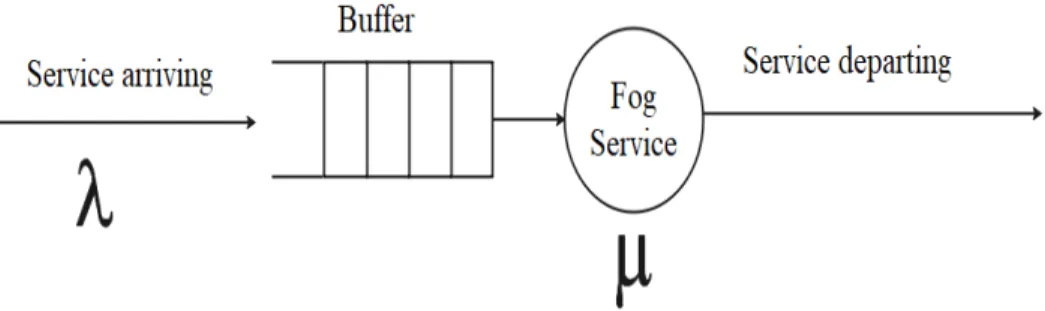
τquesi =ρ( Pw s(nρ)n n!(1−ρ)) λ−λρ (10) Whereτsi
queis the queuing timeτquefor servicesat the resources of fog nodei,λis the service rate
345
andρis the system utilisation. To compute the total time for a service in our system, its by adding the processing delay toτs
queas per Equation 11.
τcsi=τquesi + 1
µ (11)
4.3. Fog Workload
Fog workloadfwrefers to the overall usage of a fog node’s CPU (cycles/second), which is consumed
during the processing of a particular service. Thus, there are constraints on a node’s capability. This
350
leads to a limitation on the ability of processing different types of services (i.e., heavy or light). Therefore, the workload assigned to a fog node fw should not exceed the total capacity of the fog
nodefc i.
fw≤fic,∀f ∈F (12)
A service that operates on a fog node can serve several end-users in the network. Thus, the total ratio of CPU usage by the service (or services in case of parallel processing) should not exceed the
355
allocated resources allocated for a service because the allocated resources are considered to be the total fw can be handled by a fog. Equation 13 computes the total resources (rs) allocated to
pro-cess all tasksts for a services.
frss =sw= n X t=1 Cfi ts,dse ≤f i c,∀s∈S,∀t∈Ts (13)
The total fog’s workload capacity (fc) depends on the actual hardware specification of the allocated
device. The assignment variablesw(i.e., total service workload) is set so that total service processing
360
workload does not exceed fc, as per Equation 13, where C fi
ts denotes the total resource (CPU in
consumption in hertz, havinghertz=cycles/second) consumed by a service’s tasks on fog nodefi.
For more realistic scenarios, we have separate between services workloads depending on the type of service’s request type, having a heavy-weight and low-weight service’s request depends on a service’s packets size. For instance, when a service only processes small data from sensors, this will consume low
365
computational power, thus, the workload on fog is low. While, in services that performs heavy real-time video processing, the workload will be high on the fog node. Therefore, services workload (sw)
service workload multipled byλas per Equation 14. Thus, fw should be less than the fc assignment variable (i.e.,fw<=fc). 370 fw= n X x=1 swx.λs,∀s∈S (14)
4.4. Average Delay in a Fog Node
Fog node is a device located within the local network and equipped with communication protocol and computation power. We assume that nodes at the fog layer receive service packets from IoT nodes for processing and it has enough buffer size for incoming packets. Thus, the services arrival trafficλ
to fogs according to Poisson and processing rate of fog is exponentially distributed over fogs according
375
to light-services processing (µ) and heavy-services processing rate (µ0). To compute the waiting for a service on a specific fog node, it will be through calculating the total time for processing the current heavy and light services in the fog queue. For instance, to obtain the average waiting time for a services that arrived at fi it will be done through the total time consumed by fi to process
all current services. HavingnSh refer to the number of heavy-services andnSlrefer to the number of
380
light-services, Equation 15 computes the average waiting time for a newly arrived service onfi: nSh= X sfi h,∀sh∈S nSl= X sfi l ,∀sl∈S τfi sw = nSh µ0 + nSl µ (15)
It is worth to mention that, iffi queue is not empty (i.e., we havenSh+nSl6=φ), then we have
(nSh+nSl−1) mix types of services in the queue and one service is currently in processing.
4.5. Problem Formulation and Constraints
It is crucial to guarantee minimal service delay to end-users during service processing at the fog
385
layer. The four sources of delay mentioned in Figure 4 are included in the latency minimising schema. The total latency for a service sent from tn to fi is computed by adding the time of uploading a
service’s packets (τ) to the waiting time for the service in the fog queue (τque) until it gets processed.
The delay for processing the service (τproc) and the time to respond back (τ) to tn is also added
to the total latency for the service as per Equation 16. For simplification, we assume that(τ=τ),
390
having ([τ=τ]=2τ) because logically the returned packet contents normally is similar or smaller than the sent packet.
τs=τ+τques +τproc+τ,∀s∈S
τs=τques +τproc+ 2τ,∀s∈S (16)
We address the problem of having an optimal workload on fog nodes alongside with achieving minimal delay for IoT services. Thus, achieving reasonable load includes executing/processing the desired services within the threshold limit of fog capability. In addition, low latency for IoT services
395
includes delivering the services results within the required period, i.e., before service deadline (sd) with
P : min[τs]6sd,∀s∈S (17) s.t. fcmin6fw6fcmax (18) X λs6 X µf (19) Psd(n, p)>serviceLevel (20) λs min[Dp] −−−−−→fi (21) τs6sd,∀s∈S (22)
The constraints on this research are to reduce service latency. Therefore, our constraints are written with focus on achieving minimal service delay. In constraint (18), we indicate that (fw) is strictly bound
by an upper limit (fmax
c ) and lower limit (fcmin) which is related to fog capabilities based on CPU
400
frequency (unithertz). Constraint (19) imposes that the total traffic arrival rate (λs) to a fog domain
should not exceed the service rate (µf) of this fog domain. Constraint (20) imposes the probability
of directly processed services should be greater or equal to the desired service level. Constraint (21) impose the first destination for the IoT services traffic generated at the IoT Things layer will be to a fog node with minimal cost of propagation delay within the fog domain (ideally, lowest propagation
405
delay is for the nearest fog node). Finally, constraint (22) is strictly bound by the service timeτsthat
should be within the limit of service deadlinesd.
4.6. Offloading Model
The offloading model proposes to balance the load within the fog domain by distributing service traffics from the congested fog nodes to other fogs within the domain. To balance services traffic in fogs
410
domain, we assume that fogs at any giving location are reachable to each other within the same fog domain as per our network model in Section 4.1, which models the fog network as a mesh network; this assumption in line with the work in [24] and [43]. In this research, we consider a real-world scenario of services flows where services arrival rates can significantly vary from one fog node to another [24] depending on fog location, since we have λs
min[Dp]
−−−−−→ fi constraint that is services are directed to
415
nearest fog from thing for processing. For instance, in Figure 7, we demonstrate the scenario where fogs can vary in their traffic load due to their geo-location. In a similar scenario, offloading the traffic from loaded to idle fog can be crucial to mitigate the load and keep the service latency to the minimal. For example, given that only mobile vehicles are considered in traditional VANET, the authors in [34] discuss how mobile vehicles (which are loaded nodes) and parked vehicles (which are idle or semi-idle
420
nodes) should work together “as fog nodes” to transmit information and process requests to minimise the network load on mobile vehicles, increase efficiency and reduce latency.
It should be noted that the latency (time variable) and money variable have a linear relationship with each other - they impact directly on each other. For example, in intelligent transportation system discussed in [44], the vehicular communications prove reducing the traffic congestions and, hence, the
425
Round-trip Delay Time (RDT) thereof cutting down the fuel consumption (money variable). Another good example happens regularly in the financial market where having low-latency between placing an order and executing the order is crucial to get the order at the favourite price.
The decision factors where a node is congested and offloading is required significantly on fog work-load (fw), which is associated with the service traffic arrival rate (λs) and total processing rate (i.e.,
ser-430
vice rateµ) which is down to fog CPU frequency (i.e., node capability). In addition, service processing time τs, which ideally should not exceed service deadline (sd). Therefore, to make the decision of
offloading by a fog is whenτs> sd, as per Probability 23, having (Os) for offloading service decision:
Os= (
1, ifτs> sd
Loaded Fog
Semi Idle Fog
Idle Fog
City Centre Edge
City Centre
Car park
Figure 7: Loaded, idle and, semi-idle fog nodes based onλs−−−−−−→min[Dp] fi
Thus:
τs> sd,∀s∈S τques +τproc+τ> sd
In Probability 23, Os value is set to either 0 or 1, where 0 refers to no offload is required and 1
435
refers that the newly arrived service will suffer form latency and will not be able to meet the service deadlinesd. Hence, service offloading is required.
Algorithm 1 has been developed to detect the fog nodes that suffer from congestion issue, and determining the overload. The goal of this algorithm is to answer the question ofWhen to offload? and What to offload?. The first part of the algorithm (Procedure 1) determines if the fog node is congested
440
or not. This starts by getting fog queue size and queued services sorted by their types (i.e., heavy-services and light-heavy-services) as per lines 1-5. Later, lines 6-8 examine if one or more heavy-services in the queue will miss their deadlineSd, or if the service arrival rateλis bigger than the outcome of the fog
nodeµ. If any of the conditions is satisfied, a flag indicates that the node is congested as per line 9. The second part of the algorithm (Procedure 2) determines the overload by computing the number of
445
services causing the congestion as per lines 24-26. The overload Ol will hold the list of services that
requires offloading to other nodes as per lines 27-28.
To balance the services on fog nodes and achieve optimal workload and minimal service delay, we adopt the offloading to the best available node that can deliver the desired services within the scheduled time (i.e.,τ < ds). Therefore, to obtain the best node, which will handle the overload, we compute
450
the service timeτs for the services required offloading among all available nodes using Equation 24,
thus, having some constraints on the node that participate in the process to handle the overload such as load limit. min[τs] =min n X i=1 [τfi que+τ fi proc+τ] (24) s.t. fcmin 6fw6fcmax X λs6 X µf τs6sd,∀s∈S
The best available nodes are those that provide a service with minimal delay. Algorithm 2 finds the best node to handle the overload on the congested node, and than offload the overload from the
Algorithm 1:Maintain Fog Load
Input:Fog (Fi); FogCapacity (Fc); QueueSize (Qs)
Parameters :Offload (Os); OverLoad (Ol); Services (S); ServiceType (St) Initialisation:Fi=φ;Fc=φ;Qs=φ;S=φ
Result:Determine Fog overload, if any.
1 Procedure 1.Overload Threshold by
2 Fc=Fic . Fc initiate fog
3 Qs=←−getQueueSize(Fi)
4 S=list{Qs} . get list services
5 S=sort(S,bySt) 6 foreach s∈S do 7 τcsi=τquesi +1 µ 8 if (τcsi≥Sd) ||λ≥µ)then 9 setF lag(Os) = 1 10 break; 11 else 12 setF lag(Os) = 0 13 end 14 end 15 Fque=timeCostF un(s, τcs) 16 Fi←−Fque 17 return (Fi, Os) 18 End
19 Procedure 2.Determine the Overload by
20 get (Fi, Os) 21 Fc=getCapaxity(Fi) 22 µ= Fc Fi que 23 if (Os== 1 ||λ≥µ)then
24 foreach s∈Fquedo
25 S=getServices(out:s←τcs≥Sd) 26 end 27 Fque=Fque−S 28 Ol=S 29 else 30 get(Fi, Os) 31 continue 32 end 33 returnOl 34 End
congested node. In addition, the goal of the algorithm is to answer the question ofWhere to offload?.
Algorithm 2:Service Offloading
Input:FogNode (Fn); FogLoad (Fl); OverLoad (Ol). Parameters : FogCapacity (Fc); Propagation (Dp). Initialisation:Fn =φ;Fc=φ;Fl=φ;Ol=φ.
Result:Share the Overload with best available node
1 Procedure 1.Determine best available node by
2 FL=list{φ} . FL initiate fog list
3 FL=list[Fn]←−getF ogN odes(out: (Fn, Fc))
4 FL=sort(FL,byFc DESC)
5 foreach Fn∈FL do
6 if F n←−(Fl≥F cmax)then
7 FL=pop(F n) . remove busy node
8 else 9 τs= Pn i=1[τ i que+τproi +τ] 10 if (τs< sd)then 11 list.add(Fn, τs) 12 continue 13 else 14 FL=pop(F n) 15 end 16 end 17 end 18 returnFL 19 End
20 Procedure 2.Handover the Overload by
21 if FL 6=φthen 22 Fn=min[FL(τs, Dp)]) 23 Fln=Fl+Ol 24 else 25 goto:1 26 end 27 End
The first part of the algorithm (Procedure 1), shows the process of finding the best available node(s) for handling the overload pointed in Algorithm 1. Lines 2-3 of the algorithm initiate the list of active fogs in the domain alongside with the node’s capacity and current load (i.e., queue size). The list of available nodes will be refined by removing the nodes that are already busy with other services (i.e.,
460
λi=µi) as per lines 6-8. The remaining part of Procedure 1, lines 9-18 compute the time required for
a service to run on each of the available nodes. If the time is within the limit allowed for the service (i.e, beforeSd), the system will be keep the node in the list and log the expected service time against
the node as per lines 9-12. If theτsonFn is less thanSd, thanFn will be removed from the list as per
lines 13-15. The second part of the algorithm (Procedure 2), receives the list of best available nodes. If
465
the list is not empty, that means there is at least one fog able to take the overload. However, if there is more than one node in the list, the system will direct the overload to a node that can provide minimal
5. Evaluation
In this section, we evaluate through MATLAB-based simulation theF2F model, which is about
470
providing optimal fog workload with minimal latency for IoT services. A scientific and comprehensive network latency [45] has been calculated (i.e., latency of heavy packets, light packets, mixed types of packets and latency per node) to demonstrate the superior performance of the proposedF2Fmodel. We validated the results against 2 benchmark algorithms: Random Walk Algorithm (RWA) [46] [47], and Neighbouring Fogs Algorithm (NFA) [48]. Simulation settings are presented in the following subsection
475
followed by a discussion of the simulations results. 5.1. Simulation Settings
In this section, we describe the settings we adopted during the simulations. We specify the network topology, propagation and transmission delay, with link bandwidth and fog nodes capabilities, as follows:
480
• Network topology modelled as an indirect graph represents fog mesh network at the fog layer. 15 fog nodes were considered (fn = 15) and connected together through internal communication
link. Moreover, the links between nodes are weighted based on the propagation time between nodes, for instance, if Dp between f og1 and f og2 is one second, then the link weight between both nodes is (f og1←→1 f og2). Similarly, the services arrived to the fog layer are assigned to fog
485
based on the smallestDp between the node and source, which has the smallest distance. • Network bandwidth depends on the type of service. For light-packets (e.g., data packets from
sensors) the communication bandwidth is 250Kbps[49], which is equivalent to 2.0×10⁶ hertz. The communication protocol is IEEE 802.15.4, and ZigBee. For heavy-packets (e.g., data packets from cameras) the communication bandwidth is 54M bps [50], which is equivalent to 4.3×10⁸
490
hertz [50]. The communication protocol is IEEE 802.11a/g. The transmission rate between the
fog nodes is expected to be higher'100M bps[13].
• Transmission and propagation delays, the transmission delay Dt for a packet is dependent on
the packet sizelp alongside with the associated upload bandwidth b. Therefore, we impose an
average packet size that will vary according to the type of packet (i.e., heavy and light packets).
495
The average packet size for light-packets is 0.1 KB, while the average packet size for heavy-packets is 80 KB [13]. With regard to the propagation delay Dp, we use packet round trip
time (i.e.,τ) same as in [13] byτ= 0.03×ld+ 5, whereldis the distance with unit km, and τ time unit isms.
• Fog node capabilities consider the service rateµthat varies from one node to another. Fog node’s
500
capability determinants by CPU frequency, therefore nodes are variant in CPU and the rang is between 0.2 GHz to 1.5 GHz [51], which includes the CPU frequency of CISCO fog device. 5.2. Benchmarking
We considered 2 algorithms for benchmarking purposes:
1. Random Walk Algorithm (RWA) [46] [47], which imposes that arriving service requests are
505
assigned to a nearest fog node from source; if fog is congested it will offload the service randomly to another fog node. In this scenario, we assume that each fog node within the domain has the same probability of being selected.
2. Neighbouring Fogs Algorithm (NFA) [48], which is imposes that congested fog will offload the overload to the nearest fog node with bigger capacity.
510
Moreover, our comparison also includes the typical service distribution based on assigning services to the nearest node to the IoT thing with No Offloading Algorithm (NOA). We refer to our proposed algorithm as Optimal Fog Algorithm (OFA).
5.3. Results and Discussion
The performance metric we used is the average service time that reflects the efficiency of service
515
completion time (aka amount of latency). The lowest the average service time (min[τs]), the better
the efficiency of service QoS.
Figure 8 illustrates the performance of our OFA based on the average response time for all received services according to a service’s packets type. We also show a comparison between results of OFA and the results obtained from other algorithms mentioned in Section 5.2. The simulation settings for this
520
experiment is as follow:
• Fog nodes with different capabilities, hence, nodes vary in their service rateµ.
• Fog nodes capability based on CPU frequency with a minimum of 200×106 hertz, incremented by 100 hertz until it get to maximum CPU capability of 15×108.
• Service arrival rateλ= 3×10²packet per second as in [24], andλis fixed during the experiment
525
to ensure all algorithms have the same traffic arrival rate.
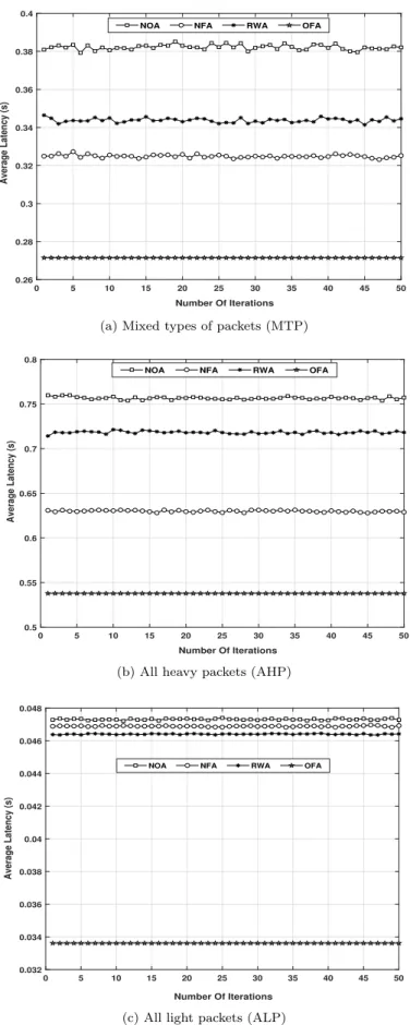
Figures 8a, 8b, and 8c are grouped by packet type (heavy-packets versus light-packets). In Figure 8a, the packets type is mixed (MTP), having a random number of heavy and light packets. However, the random number is fixed through out the experiment to ensure consistency across all algorithms. In Figures 8b and 8c, the packets are set to either all heavy-packets (AHP) or all light-packets (ALP).
530
This is to examine the performance based on different scenarios. In Figure 8 the vertical line represent the average latency per algorithm to serve all arrived services, and the horizontal line is the number of iterations carried out to insure that the obtained results are consistent and not random. It is clear that OFA has the lowest service latency among other algorithms through all iterations and with all types of packets. NOA also has the lowest service time because it does not consider offloading when a
535
node becomes congested. Hence, we end-up having a small node capacity with large queue size (i.e.,
µi< λi), and a large node capacity with low queue size. The performance of RWA and NFA are better
than NOA but still hither than our OFA. However, RWA has the worst performance with MTP and AHP as it randomly offloads the overload, which is relatively blind algorithm as it not considered the current load (fw) and propagation delay (Dp).
540
The next simulations were conducted based on service latency per fog node. Similar to previous experiments, we use fog nodes with different capabilities based on CPU frequency with a minimum of 200×106 hertz, incremented by 100 hertz until it gets to maximum CPU capability of 15×108 (i.e, Fn = 14). In this simulation, we increment the service arrival rate so, that, the total packet received
is 1 million service as in [13]. The packet type in this experiment is mixed with a random number
545
of heavy-packets and light-packets. Figure 9 shows the average latency per fog node. It is clear that OFA achieves a consistent average latency. In contrast between OFA, on the one hand, and with NFA and RWA, on the other hand, OFA has the lowest average latency between nodes 1 to 7, but greater average latency from node 8, and thereafter. However, the average latency differences is much higher for NFA and RWA in comparison to OFA for nodes from 1 to 7 compared to the average latency
550
differences from node 9 to 14. This difference accrues as OFA workload distribution strategy, OFA tries to achieve balanced service distribution based on node capacity. Therefore, the work assigned to nodes considers the overall capacity and current load before offloads a request, while NFA and RWA are relatively blind in this manner. Hence, OFA achieves almost consistent latency on each individual node, while the average latency for NFA and RWA vary and are inconsistent.
555
To prove the optimal distribution of packet with OFA we run a new experiment and recall the settings from the previous experiment. However, in this experiment, the vertical line represents service usage (i.e., number of packets) as per Figure 10. The nodes are sorted from smallest capacity (i.e., lowest CPU) to largest (i.e., largest CPU), having the first node with 200×106hertz and node 14 with 800×106 hertz. It is clear that the packets distribution with OFA is completely different than NFA and RWA
560
as it distributes packets according to the node capacity. Hence, the first node receives less number of packets and the last node receives more number of packets. In comparison with NFA and RWA, the
0 5 10 15 20 25 30 35 40 45 50 Number Of Iterations 0.26 0.28 0.3 0.32 0.34 0.36 0.38 0.4 Average Latency (s)
NOA NFA RWA OFA
(a) Mixed types of packets (MTP)
0 5 10 15 20 25 30 35 40 45 50 Number Of Iterations 0.5 0.55 0.6 0.65 0.7 0.75 0.8 Average Latency (s)
NOA NFA RWA OFA
(b) All heavy packets (AHP)
0 5 10 15 20 25 30 35 40 45 50 Number Of Iterations 0.032 0.034 0.036 0.038 0.04 0.042 0.044 0.046 0.048 Average Latency (s)
NOA NFA RWA OFA
(c) All light packets (ALP)
1 2 3 4 5 6 7 8 9 10 11 12 13 14 Fog Nodes 0 1 2 3 4 5 6 7 Average Latency (s)
NOA NFA RWA OFA
13 14
0.5 1 1.5
Figure 9: Average latency per node
packet distribution on average is steady among all nodes regardless of the node capacity, which causes the issue of latency as, on the one hand, nodes with small CPU frequency consumes significant time to process all received packets. While, on the other hand, nodes with large CPU frequency have already
565
finished processing the received packets as per Figure 9.
Figure 11 shows the impact of increasing the number of packets on latency. During simulation, service’s packets are varied from one packet to 10×104packets in Figure 11a; thus, the packet type is fixed to heavy-packet for consistency. The service utilisation rate is incremental parameter from 1% to 100%, thus, this rate is fixed at any given timestamps, for example, if the service utilisation rate is 50%,
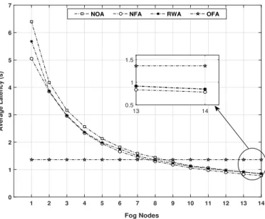
570
all algorithms; OFA, NAF, RWA, and NOA will receive the same rate. It is obvious that increasing the number of arrived packets (i.e., increase the service arrival rateλ) will increase the overall latency. The total latency and performance of the algorithms vary; OFA has the lowest service latency as per Figure 11a. The service latency is stable with small delay of approximately 0.6 second for the received packets upto 6.5×10⁴, thereafter, the latency start to increase significantly for NOA, RWA, and NAF.
575
While, OFA remains stable with less than 1.2 second latency for all received packets and upto 10×104 packet. Moreover, in Figure 11b, we have increased the packets utilisation to 10×106 to show the continues of latency variations for the different algorithms compared to OFA. It is clear that OFA has a sustainable packets processing with the increases of service’s packets (i.e., high traffic), in term of latency, as it has the lowest packet’s latencies.
580
From previous simulations we increase the packet arrival rate λ to 15×104 to monitor how the offloading performance and service latency will be effected. Latency will be increased for all offloading algorithms. However, the incremental rate will matter as this will reflect the sustainability of the offloading algorithm. Figure 12 shows the maximum and average latencies for the 15×104 packets (with type heavy) based on the offloading algorithms. In comparison between the maximum latencies
585
for all offloading algorithms in Figure 11 and 12, it is clear that the increment of maximum latency for NFA, NOA, and RWA is significantly more than the maximum latency for OFA, as in Figure 11 the maximum latency for a packet with OFA is around 0.6 second, and in Figure 12 the maximum latency is 0.8 second. Whereas, within NFA and RWA the maximum latency is 1.5 and 2 seconds, respectively, in Figure 11, while the maximum latency is 2.7 and 3.2 seconds, respectively, in Figure 12. It is clear
590
that the latency incremented by approximately more than 1 second with NFA and RWA offloading algorithm, while the latency increment for OFA is only 0.2 second.
1 2 3 4 5 6 7 8 9 10 11 12 13 14 Fog Nodes 0 0.5 1 1.5 2 2.5 3 3.5
Packets Load (#Cycles)
109
NOA NFA RWA OFA
Figure 10: Average load on nodes
6. Conclusions and Future Works
Although fog computing is recognized as a computing model that suits IoT, it is still not widely used. Due to the spatial and temporal dynamics of IoT things distribution, the computations loads on
595
fogs significantly vary. Thus, nodes could be lightly loaded, while others are not causing fog congestion then, latency. In this paper, we propose a novel Fog Resource manAgeMEnt Scheme (FRAMES) that justifies fog distributions and management with service load allocation and computing load allocation via service offloading among fog nodes to achieve minimal latency for IoT services. We propose a feasible solution that enables fog traffic management via service offloading in fog-based architecture
600
that serves the purpose of minimizing the average response time for real-time IoT services. Through the extensive experiments, it is clear that the offloading significantly impacts the overall latency of services. A proper resources managements with accurate offloading algorithm will significantly reduce service latency and, the number of fog nodes and it’s capacities will also impact service latency. Moreover, it is clear that the proposed OFA has the lowest service response time in comparison with RWA and NFA.
605
OFA and have the potential in achieving sustainable network paradigm to highlights the significance and benefits of adopting fog computing paradigm. In our future work, we plan to extend the simulation using a data processing techniques (such as MapReduce or Spark) with a real dataset to evaluate the Fog-2-Fog model. In addition, we plan to study security issues that associate with malicious fogs since it has been considered as a critical infrastructure. Thus, develop a secure fog layer that defend
610
users and services privacy, also perform security tests to understand the robustness against malicious attacks, particularly in theFog-2-Fog model.
[1] R. Deng, R. Lu, C. Lai, T. H. Luan, and H. Liang. Optimal workload allocation in fog-cloud computing toward balanced delay and power consumption. IEEE Internet of Things Journal, 3(6):1171–1181, Dec 2016.
615
[2] Mohammed Al-khafajiy, Lee Webster, Thar Baker, and Atif Waraich. Towards fog driven iot healthcare: Challenges and framework of fog computing in healthcare. InProceedings of the 2Nd International Conference on Future Networks and Distributed Systems, ICFNDS ’18, pages 9:1– 9:7, New York, NY, USA, 2018. ACM.
[3] Qi Zhang, Lu Cheng, and Raouf Boutaba. Cloud computing: state-of-the-art and research
chal-620
6.5 7 7.5 8 8.5 9 9.5 10 Packet Index 104 0.5 1 1.5 2 2.5 3 Latency (s)
NOA NFA RWA OFA
9.95 9.96 9.97 9.98 9.99 10 104 1 1.5 2 2.5
(a) Packet index upto 104
8.4 8.45 8.5 8.55 8.6 8.65 8.7 8.75 8.8 8.85 8.9 Packet Index 106 2.4 2.6 2.8 3 3.2 Latency (s)
NOA NFA RWA OFA
(b) Packet index upto 106to show the variations
Figure 11: Latency per packet
[4] W. Kim and S. Chung. User-participatory fog computing architecture and its management schemes for improving feasibility. IEEE Access, 6:20262–20278, 2018.
[5] Lizhe Wang, Gregor von Laszewski, Andrew Younge, Xi He, Marcel Kunze, Jie Tao, and Cheng Fu. Cloud computing: a perspective study. New Generation Computing, 28(2):137–146, Apr 2010.
625
[6] J. Sun, G. Zhu, G. Sun, D. Liao, Y. Li, A. K. Sangaiah, M. Ramachandran, and V. Chang. A reliability-aware approach for resource efficient virtual network function deployment. IEEE Access, 6:18238–18250, 2018.
[7] Gang Sun, Victor Chang, Guanghua Yang, and Dan Liao. The cost-efficient deployment of replica servers in virtual content distribution networks for data fusion.Information Sciences, 432:495–515,
630
2018.
[8] Friedemann Mattern and Christian Floerkemeier.From the Internet of Computers to the Internet of Things, pages 242–259. Springer Berlin Heidelberg, Berlin, Heidelberg, 2010.
NFA NOA OFA RWA 0 0.5 1 1.5 2 2.5 3 3.5 4 4.5 Maximum Latency (s)
Figure 12: Maximum latency upon heavy-packets
[9] M. Al-khafajiy, T. Baker, A. Waraich, D. Al-Jumeily, and A. Hussain. Iot-fog optimal workload via fog offloading. In2018 IEEE/ACM International Conference on Utility and Cloud Computing
635
Companion (UCC Companion), pages 359–364, Dec 2018.
[10] Cisco Systems. Fog computing and the internet of things: Extend the cloud to where the things are, 2016.
[11] D Evans. The internet of things: How the next evolution of the internet is changing everything. Cisco Internet Business Solutions Group (IBSG), 1:1–11, 01 2011.
640
[12] Q. Fan and N. Ansari. Towards workload balancing in fog computing empowered iot. IEEE Transactions on Network Science and Engineering, pages 1–1, 2018.
[13] A. Yousefpour, G. Ishigaki, R. Gour, and J. P. Jue. On reducing iot service delay via fog offloading. IEEE Internet of Things Journal, 5(2):998–1010, April 2018.
[14] Saeed Khanagha, H.W. Volberda, and Ilan Oshri. Business model renewal and ambidexterity:
645
Structural alteration and strategy formation process during transition to a cloud business model. R and D Management, 44, 06 2014.
[15] Flavio Bonomi, Rodolfo Milito, Jiang Zhu, and Sateesh Addepalli. Fog computing and its role in the internet of things. InProceedings of the First Edition of the MCC Workshop on Mobile Cloud Computing, MCC ’12, pages 13–16, New York, NY, USA, 2012. ACM.
650
[16] M. Al-khafajiy, T. Baker, H. Al-Libawy, A. Waraich, C. Chalmers, and O. Alfandi. Fog com-puting framework for internet of things applications. In 2018 11th International Conference on Developments in eSystems Engineering (DeSE), pages 71–77, Sep. 2018.
[17] Amandeep Singh Sohal, Rajinder Sandhu, Sandeep K Sood, and Victor Chang. A cybersecurity framework to identify malicious edge device in fog computing and cloud-of-things environments.
655
Computers & Security, 74:340–354, 2018.
[18] Safa Otoum, Burak Kantarci, and Hussein Mouftah. Adaptively supervised and intrusion-aware data aggregation for wireless sensor clusters in critical infrastructures. In2018 IEEE International Conference on Communications (ICC), pages 1–6. IEEE, 2018.
![Figure 7: Loaded, idle and, semi-idle fog nodes based on λ s min[D p ]](https://thumb-us.123doks.com/thumbv2/123dok_us/1370983.2683592/17.918.185.731.125.374/figure-loaded-idle-semi-idle-fog-nodes-based.webp)