Flex-Ro: A Robotic High Throughput Field Phenotyping System

(1)

DigitalCommons@University of Nebraska - Lincoln

Biological Systems Engineering--Dissertations,

Theses, and Student Research Biological Systems Engineering

12-2019

Flex-Ro: A Robotic High Throughput Field Phenotyping System

Joshua N. Murman

University of Nebraska-Lincoln, [email protected]

Follow this and additional works at: https://digitalcommons.unl.edu/biosysengdiss

Part of the Bioresource and Agricultural Engineering Commons

Murman, Joshua N., "Flex-Ro: A Robotic High Throughput Field Phenotyping System" (2019). Biological Systems Engineering--Dissertations, Theses, and Student Research. 99.

https://digitalcommons.unl.edu/biosysengdiss/99

This Article is brought to you for free and open access by the Biological Systems Engineering at

DigitalCommons@University of Nebraska - Lincoln. It has been accepted for inclusion in Biological Systems Engineering--Dissertations, Theses, and Student Research by an authorized administrator of

(2)

FLEX-RO: A ROBOTIC HIGH THROUGHPUT FIELD PHENOTYPING SYSTEM by

Joshua Nathanael Murman

A THESIS

Presented to the Faculty of

The Graduate College at the University of Nebraska-Lincoln In Partial Fulfillment of Requirements

For the Degree of Master of Science

Major: Agricultural and Biological Systems Engineering Under of the Supervision of Professor Santosh K. Pitla

Lincoln, Nebraska December 2019

(3)

FLEX-RO: A ROBOTIC HIGH THROUGHPUT FIELD PHENOTYPING SYSTEM Joshua Nathanael Murman, M.S.

University of Nebraska, 2019 Advisor: Santosh K. Pitla

Research in agriculture is critical to developing techniques to meet the world’s demand for food, fuel, fiber, and feed. Optimization of crop production per unit of land requires scientists across disciplines to collaborate and investigate new areas of science and tools for data collection. The use of robotics has been adopted in several industries to supplement labor, and accurately perform repetitious tasks. However, the use of autonomous robots in commercial agricultural production is still limited. The Flex-Ro (Flexible structured Robotic platform) was developed for use in large area fields as a multipurpose tool to perform monotonous agricultural tasks.

This work presents the design and implementation of the control system for the Flex-Ro machine. The machine control architecture was developed for safe operation with redundant emergency stops and checks. Operators use the remote-control device to maneuver the machine in uncontrolled environments. Autonomous field coverage was developed using global positioning system (GPS) guidance. The guidance system tracked within 4 cm of the guidance line 95% of the time at a travel speed of 4 kph. Waypoint guidance was implemented and demonstrated such that Flex-Ro could be programmed to follow complex paths and curves.

(4)

High-throughput plant phenotyping is a continuously developing and evolving field of plant science. The methods used to collect phenotyping data include drones, satellites, manual measurement, and ground rovers. A suite of phenotyping sensors was installed onto the Flex-Ro to cover large field areas. The system was verified in soybean research plots at the University of Nebraska-Lincoln (UNL) Spidercam phenotyping facility. Positive correlations between the Spidercam and Flex-Ro phenotyping data were established. The Flex-Ro was able to statistically distinguish between soybean variety emergence and maturity differences. The late season phenotyping data showed statistical differences between the fully irrigated versus deficit plots. Basic economic calculations estimated the cost to operate the Flex-Ro machine for field phenotyping use at approximately $5.50/ha.

(5)

Acknowledgments

I would first like to thank my advisor, Dr. Santosh K. Pitla, for encouraging me to take this next educational step. Thank-you for your guidance and mentorship through this process.

Thank-you to my graduate committee members Dr. Yufeng Ge and Dr. Joe D. Luck for their support.

Thank-you to the University of Nebraska Agricultural Research Division for support and use of Spidercam field space to test Flex-Ro. Thank-you to David Scoby and Geng ‘Frank’ Bai for collecting and processing the Spidercam phenotyping data.

Thank-you to the in-kind donors to the Flex-Ro machine; Kubota Engine America supported by Anderson Industrial Engines, ifm efector inc., and Danfoss Power Solutions.

Finally, thank-you to my parents, Craig and Deb, for always supporting me and for teaching and continuously exemplifying to me the values of faith, work ethic, and character.

(6)

Figure 1.1: Phenotyping and crop-breeding cycle. Scale and resolution of developed phenotyping platforms (Source: Shakoor et al., 2017). ... 5 Figure 2.1: Remote control box developed for teleoperation of the Flex-Ro platform. ... 18 Figure 2.2: CAN node layout on the Flex-Ro platform. Dashed wire shows connection via J1939 CAN bus. ... 20 Figure 2.3: Main operating screen of the Flex-Ro remote. Danfoss DP600TM display. . 23 Figure 2.4: Left - Remote diagnostics screen. Right - Remote steering calibrate screen. 24 Figure 2.5: Main application tab for the FlexRoRun application. Developed using

MATLAB App Designer. ... 27 Figure 2.6: Navigation tab within the FlexRoRun application. Developed using the MATLAB App Designer. ... 28 Figure 2.7: Lateral error (perpendicular distance) at point C from line defined by points A and B. ... 35 Figure 2.8: Heading error as a function of machine heading. Discontinuities at vertical lines. ... 37 Figure 2.9: Vehicle coordinate system convention with respect to geographical north. .. 39

(11)

Figure 2.10: Left: Conventional front wheel steer headland turn. Right: Traverse

headland navigation method. ... 42 Figure 2.11: ifm O3M 151 3D Smart Sensor installed on the front of the Flex-Ro

platform. ... 44 Figure 2.12: CAN message output from one object detected by ifm O3M 151 3D Smart Detector. Viewed and decoded on Vector CANalyzer software. ... 46 Figure 2.13: One of four red e-Stop buttons located on exterior of machine for quick and safe access. ... 49 Figure 2.14: Testing AB line navigation in corn stubble. ... 52 Figure 2.15: Lateral error over time, automatically tracking on level field ground at 3.7 kph... 53 Figure 2.16: Automatic waypoint path following and lateral error over time. Coordinates translated to where data recording was initialized. ... 55 Figure 2.17: Recorded GPS data for front wheel headland turn (left) and four-wheel crab headland traverse (right). Coordinates translated to where data recording was initialized. ... 57 Figure 2.18: Mean error magnitude at obstacle set position recorded by ifm O3M 151 3D Smart Sensor. ... 58

(12)

Figure 2.19: Dynamic obstacle approach test. Stopping distance was measured from detector on front to board. ... 59 Figure 2.20: Measured distance from obstacle after machine automatically stops due to detected potential collision. ... 60 Figure 3.1: PhenoBar mounted to the Flex-Ro machine. Three sensor units cover a 4.5m swath. ... 65 Figure 3.2: PhenoBox installed with laptop tray which contains data acquisition hardware for the Flex-Ro phenotyping system. ... 67 Figure 3.3: LabVIEW front panel used as the phenotyping data acquisition system for the Flex-Ro. ... 69 Figure 3.4: Custom PhenoCalc application Field Summary tab to process raw Flex-Ro captured data. ... 70 Figure 3.5: Custom PhenoCalc application Plot Summary tab used to parse per plot data from large matrix. ... 71 Figure 3.6: The Flex-Ro collecting data 67 days after planting (DAP). Each of the sensor units are positioned directly over a row. ... 73 Figure 3.7: Correlation between Flex-Ro and Spidercam measured crop plot average height... 75

(13)

Figure 3.8: Temporal comparison of crop plot height averages per treatment with

different measurement techniques. ... 76 Figure 3.9: Average plot height over time per genotype with full irrigation treatment as recorded by the Flex-Ro platform. ... 77 Figure 3.10: Correlation between Flex-Ro and Spidercam measured NDVI and linear correlation. ... 78 Figure 3.11: Temporal comparison of NDVI split into the two field treatments comparing phenotyping systems. ... 79 Figure 3.12: NDVI (750-705 nm) as calculated from Flex-Ro data per genotype with full irrigation treatment. ... 80 Figure 3.13: Examples showing result of image segmentation to calculate GPF.

Segmented 'non-green' pixels shown in orange for clarity. ... 81 Figure 3.14: Correlation between Flex-Ro and Spidercam calculated crop canopy

coverage. ... 82 Figure 3.15: Temporal comparison of canopy coverages split into field treatments

comparing phenotyping systems. ... 83 Figure 3.16: Canopy coverage calculated from Flex-Ro data over time per genotype with full irrigation treatment. ... 84

(14)

Figure 3.17: Flex-Ro in the Spidercam research field collecting data at 117 DAP.

Differences in maturity can clearly be seen between plots. ... 86 Figure 3.18: Correlation coefficient of plot canopy coverage to yield over time of the Flex-Ro and Spidercam. ... 87 Figure 3.19: Correlation coefficient of phenotype data measured by the Flex-Ro to plot yield... 88 Figure 4.1: Left: Farmobile PUC data streaming device. Right: Kvaser Memorator Pro 2xHS v2 CAN logger. ... 93 Figure 4.2: Recorded distribution of machine speed between Spidercam research field and concrete track. ... 96 Figure 4.3: Economics of Phenotyping operation using the Flex-Ro machine with a swath width of 18.3 m and data collection cycle time of 8 sec. ... 97

(15)

Table of Tables

Table 2.1: List of control system hardware used on the Flex-Ro machine. ... 19

Table 2.2: Engine control message. Start and Length shown as Byte.bit ... 29

Table 2.3: Hydrostatic drive pump control message. Start and Length shown as Byte.bit ... 30

Table 2.4: Steering control messages. Start and Length shown as Byte.bit ... 32

Table 2.5: Example status message. Start and Length shown as Byte.bit ... 33

Table 3.1: List of sensors installed in each unit on the Flex-Ro PhenoBar. ... 66

Table 3.2: Results of testing for statistical difference in recorded phenotyping data means of the SPC and Flex-Ro phenotyping systems. ... 85

Table 3.3: Genotypes and irrigation treatments. ' - soy seed brand 1, " - soy seed brand 2. ... 85

Table 3.4: Correlations between recorded data and final plot yield with significance level. ... 87

(16)

Table of Equations

Equation 2.1: Perpendicular offset from navigation line calculated from three points, where A and B define the navigation line ... 36 Equation 2.2: Applying the sign of lateral error based on the line (AB) and current points. ... 36 Equation 2.3: Predicting the object’s position with respect to the machine’s x coordinate. ... 47 Equation 2.4: Predicting the object’s position with respect to the machine’s y coordinate. ... 47 Equation 2.5: Calculating the machine stopping distance given the current velocity. ... 47 Equation 3.1: Calculating the NDVI using the magnitude of reflectance at 705 and 750 nm. ... 72 Equation 4.1: Calculation of the slip percentage as a ratio of velocity on concrete (vc) and soil (vs). ... 96

(17)

Chapter 1 Introduction

The agricultural industry supports the world’s needs for food, feed, fiber and fuel. Global economic and population growths are projected to increase by over 40 percent by 2050 (Bruinsma, 2009; USDA, 2019). This translates to a corresponding increase in global agricultural production by 70 percent. There are two ways to increase crop production, more yield per area or expansion of farmable land (Bruinsma, 2009). During this period of growth, the planted acres within the United States is projected to remain steady (USDA, 2019). Plateaued commodity prices with increasing input costs are driving thin margins, and limited land requires increased productivity per area. As a result, continuous research on optimization of resources is paramount to the success of modern farming operations.

1.1 Research in Agriculture

Agricultural research supports the development of efficient crop production systems. Research institutions receive grants to support work investigating cause and effect relationships across all aspects of the agriculture industry. The findings are presented to the public via extension outreach of the universities, allowing the producers to implement discoveries.

Farmers must balance costs to benefits to maximize production while maintaining profitable operation. Costs incurred during the growing season include tillage, nutrient application, seed, pesticides, herbicides, irrigation, and harvesting operations. Each one

(18)

of these items affects the output or yield of the crop. Research is conducted across all aspects of the farming operation, which seeks to draw correlations between variable inputs to outputs. Scientists from many disciplines find applicable research questions in the agricultural industry. An abridged list includes soil scientists, agronomists,

economists, engineers, entomologists, geneticists, plant breeders, statisticians, traders, financial analysts and computer scientists. Each of these stakeholders hold a position within the agricultural value ecosystem and can benefit from effective research.

There are two desired outcomes for a successful research program related to agricultural production. First is increased yield (revenue) and the second is reduced inputs (cost). Management practices must balance revenue with costs to remain profitable. For example, excessive nutrient application would increase crop output; however, the

increased costs may not be recouped with proportional yield gain (Cassman, 1999). There are non-financial implications to farming management practices also. Environmental concerns from chemical misuse is one example. Successful agricultural research ideally benefits all stakeholders of the agricultural value chain. One particularly important subset of agricultural research is the development of desirable plant characteristics.

1.1.1 Plant Breeding

Plant breeding is the method of developing crops to achieve desirable characteristics (Atefi, 2019). The current rate of increased plant productivity must continue to rise to meet the demands of the world (Araus and Cairns, 2014). Plant breeding targets increasing yield and key traits for harvestability and marketability (Fehr, 1991). For

(19)

example, a corn plant should have a high yield with strong stalks, deep roots and disease resistance. Plants resistant to insects and disease require fewer pesticides and plant traits for drought tolerance are desirable in many locations.

Plant breeding success relies on both qualitative and quantitative data. Traditionally, the breeders developed plants by visually selecting the best from each generation (Fehr, 1991). This process would be repeated several times until the desired output was achieved. New methods in genetics provide ways to accelerate breeding progress, and better target desired traits (Fahlgren et al., 2015; Fehr, 1991).

Accelerating the progress of plant genetic development is critical to meeting the world demand for increased production of food, feed, fiber, and fuel. Even with the science of molecular breeding, rapid characterization of a plant’s physical response given its genotype to an environment is still limited (Atefi, 2019). Objective quantification and qualification of phenotypic data is crucial to developing plants with the most desirable traits (Fahlgren et al., 2015).

1.1.2 Phenotyping

Phenotyping is the characterization of a plant’s physical and performance related traits (Dhondt et al., 2013). Plant breeders collect this data for genotypes in specific

environments. Leaf area index, leaf number, canopy temperature, water content, vegetative indices, canopy coverage, and stem diameter are examples of physical traits measured or calculated. The environments may be controlled, uncontrolled or measured (Dhondt et al., 2013).

(20)

Plants respond uniquely to different environmental conditions (Atefi, 2019). Plant breeders and production farmers can leverage early prediction of crop output. Plant breeders use early season phenotype data to draw preliminary conclusions on a genotype to begin developing the next generation (White et al., 2012). Yield relationships to early season phenotyping data can be statistically established. With this method, farmers marketing crop futures contracts would have a better estimate of yields and total production.

Development of reliable correlations of a plant phenotype to environmental conditions and genotypes requires extensive datasets. Long term studies are often conducted in semi-controlled research fields or controlled greenhouses with installed phenotyping systems (Foix et al., 2015). Destructive methods of measuring plant characteristics have previously been used, but limit the temporal data collection (Furbank and Tester, 2011). Large sample sizes are needed to achieve representative growth curves of a genotype. Non-destructive phenotyping uses sensors and imaging techniques to directly measure or capture data which can be used to calculate plant characteristics. These sensors can be mounted to devices for high-throughput data collection. Advancements in computational processing capacity have enabled rapid phenotyping of large populations. Current high-throughput techniques maintain high correlation to ground truth measurements (Bai et al., 2016).

Incoporating high throughput phenotyping into the plant breeding cycle will facilitate the increase in crop productivity needed to match global demands (Furbank and Tester, 2011). Phenotyping research is being developed on resolutions from plant to field level.

(21)

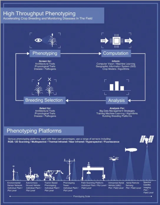
Each scale has benefit to plant breeders and crop consultants who make management decsisons based on the current state of the crop. Shakoor et al., (2017) illustrated the plant breeding cycle and scales Figure 1.1.

Figure 1.1: Phenotyping and crop-breeding cycle. Scale and resolution of developed phenotyping platforms (Source: Shakoor et al., 2017).

(22)

1.2 Use of Technology in Agriculture

Technology has been continuously incorporated into agriculture to improve the production system. Mechanization from horse to tractor revolutionized the farming industry. Machine features became more complex as technology continued to develop, and operating stations were increasingly designed for ergonomics and comfort. Electronic incorporation into agricultural machinery began with the release of a planting population monitor by DICKEY-john (Stone et al., 2008). Serial communication was first used to simplify connections to implements. Progress towards standardizing communication on a machine controller area network (CAN) bus began in the 1980’s (Stone et al., 2008). A standardized high-level CAN protocol (message format) allowed for the continued development of agricultural technologies and paved the way for brand agnostic devices. 1.2.1 The Rise of CAN bus

CAN bus technology for off-highway machinery led to the development of complex machinery systems. Multiple electronic control units (ECUs) were used to control the subsystems of machine. Electronic displays and switches in the cab required

communication with the ECUs. The Society of Automotive Engineers (SAE) and American Society of Agricultural Engineers (ASAE) jointly developed SAE J1939 as a response to the need to standardize communication protocol on off-highway machinery (Marx, 2015). J1939 defined this high-level message structure (application layer) for communication on the two wire twisted pair CAN bus (physical layer). Control, interface, and diagnostic messages were defined within the standard’s application layer. Processor

(23)

advancement preceded development of the virtual terminal (VT) which integrated machine and implement controls onto a user interface display (Stone et al., 2008). As global position system (GPS) accuracy continued to improve, the use of the VT expanded to include automatic steering applications (Buick, 2006).

1.2.2 Navigation Systems

GPS technology became prevalent on agricultural machinery first with the

implementation of precision mapping, and later automatic steering control. The turn of the century led to rapid advances in GPS hardware development and accuracy

(O’Connor, 1997). Research by O’Connor (1997) and Bell (1999) developed steering control systems based on GPS location. As time progressed, GPS hardware became more accessible and overall decreased cost of systems led to a shortened return on investment time (Buick, 2006). Automatic guidance improved field coverage efficiency by reducing overlap. Modern navigation systems have repeated accuracy of +/- 2.5 cm by using real-time-kinematic (RTK) corrections for the GPS signal (Baillie et al., 2018).

The development of automatic navigation control systems led to the delivery of other related operations. Automatic swath guidance has been extended to provide headland turn coverage (Baillie et al., 2018). Total machine automation controls the tractor and

implement through the turn, disengaging and restarting the operation on the next swath. Machine cooperation (e.g. leader and follower) technologies have been developed as a progression of automatic navigation (Thomasson et al., 2018). The current state-of-the-art technologies are operator assisted automation, or level 3 (out of 5) automation as defined

(24)

by Case IH (CNH Industrial America LLC, Burr Ridge, IL). The operator must remain in the cab ready to resume control in case of unexpected events or encounters (Case IH, 2018). Future development towards full autonomy will need to include advanced path planning and obstacle detection and avoidance (Baillie et al., 2018; Bell, 1999).

1.3 Robotics in Agriculture

The use of robotics in agriculture, while still commercially limited, is seeing rapid development (McAllister et al., 2019). Robots are designed to relieve operators of long working days and reduce overall manual labor (Werner, 2016). The use of robotics in precision agriculture increases management resolution by working unattended for long hours. Further, a smaller size compared to traditional machinery reduces soil compaction (Godoy et al., 2012).

Agricultural robots have been developed in several configurations. The use of battery power is common for smaller scale platforms (Bak and Jakobsen, 2004; Bangert et al., 2015; Griepentrog et al., 2012; Slaughter et al., 2008). However, sole electric power has runtime limitations due to the required time to charge (Werner, 2016). Internal

combustion robotic platforms have also been developed for agricultural use (Godoy et al., 2012; Werner, 2016). Petroleum powered robots have the advantage of long run times paired with short refueling periods. However, a combustion engine requires increased maintenance compared to an electric drivetrain. In either case, digital systems must be able to control all aspects of the vehicle.

(25)

1.3.1 Agricultural Robotic Control Systems

The development of autonomous agricultural robots includes research on control system methodologies. Robotic control systems are developed similar to subsystems

implemented on machinery (Troyer, 2017). Autonomous operation consists of four main stages. A machine must start with route planning. This may be present as algorithms on the machine or be pre-defined and uploaded. Coverage strategies are optimized for maximum field efficiency (J. Jin and L. Tang, 2010). The route is then augmented with environment data during operation, most commonly to avoid obstacles. After the current route is accepted, the trajectory and speed of the machine is determined. Finally, local feedback control manages the actuators of the robot to the desired operating state (Paden et al., 2016).

Robotic steering controllers are designed from a kinematic or dynamic model of the machine. Kinematic models, while less computationally expensive, are limited to slower speed operation (Bell, 1999). Advanced dynamic control methodologies can improve performance on machines which encounter a lot of variability (Uzunsoy, 2018). Different implements, payloads, and operating speeds contribute to steering controller performance (Lakkad, 2004). Simulations are used to verify controller functionality and test different scenarios without the need for the physical machine (Lakkad, 2004; Tu, 2013). The control system must compensate for variations in terrain to track the navigation line (Cariou et al., 2009).

(26)

Robots operating in uncontrolled environments may encounter obstacles at any time. Obstacle detecting sensors are installed in order to reduce the likelihood of collisions. (Emmi et al., 2014). Several methods of obstacle detection have been researched and evaluated. Methods include LiDAR’s (Biber et al., n.d.) infrared (IR) sensor (Pitla et al., 2010a) and lasers (Oftadeh et al., 2013). Accurate detection and classification of

obstacles within the field environment will be important for large scale deployment. Robotics in production agriculture are likely to manifest as several small robots operating in cooperation (Emmi et al., 2014; McAllister et al., 2019; Pitla et al., 2010b). Modular robots would be added depending on the need of the operation (Emmi et al., 2014). Swarm control architecture depends on the task. Equal distribution of work is well suited to seeding type applications, and leader-follower architecture is more suited to harvest operations (Pitla et al., 2010b).

Substantial amounts of data must be transferred between the subsystems of the robot and between the units in the swarm. CAN bus communication provides a method for handling messages within the on machine network (Baek et al., 2008). Communication between robots within the field will facilitate job coordination (Pitla et al., 2010b). Robust

network systems and relaying information to the master controller will allow the robots to be adaptable wide variety of applications.

1.3.2 Ag. Robotic Applications

There are many applications in agriculture which are well suited to robotics. The first adaptation will replace labor intensive repetitive tasks (Emmi et al., 2014). Robots

(27)

currently developed are low power and designed for non-ground engaging activities. These include targeted mechanical weeding (Åstrand and Baerveldt, 2002), precision spraying (Bangert et al., 2015), and crop scouting (Bangert et al., 2015; Shafiekhani et al., 2017)

Slaughter (2008) authored a state-of-the-art review of robotic weeding technologies. Several different methods were described as ways autonomous rovers managed weeds. Since then commercialized technologies have been developed. EcoRobtix (ecoRobotix ltd, Yverdon-les-Bains, Switzerland) Naïo Technologies (naïo Technologies Escalquens, France) and FarmWise (FarmWise Labs, Inc. San Francisco, CA) are all examples of autonomous weeding prototypes which appear available in the commercial sector. Crop scouting traditionally is completed by a trained agronomist. The agronomist must balance productivity with resolution of field coverage. Agronomists data supplements producers in decision making about crop inputs and applications. Plant phenotyping uses scouting data to draw correlations to a genotype given the measured or controlled

environment.

1.3.3 Ag Robotic Phenotyping

Phenotypic data collection is laborious. Several concepts and prototypes have been developed and implemented to facilitate high-throughput phenotyping. Phenotyping platforms vary in scale and resolution as seen previously in Figure 1.1. Data captured from unmanned aerial vehicles and satellites is used to measure broad areas on plot and

(28)

field level resolution. Ground vehicles and devices collect higher resolution data, from plot to individual plant (Shakoor et al., 2017).

High throughput ground based phenotyping platforms were first developed on manual push carts. White and Conley (2013) and Bai et al. (2016) instrumented carts to measure plot level phenotypic traits. The use of carts enabled multiple sensor mounting

configurations and cover more area as a result. A stop-measure-go technique was used for plot coverage and is well suited to manual operation of the cart (Bai et al., 2016). Strong correlations were established to ground truth measurements to prove the viability of the cart phenotyping system.

The development of phenotyping carts enabled faster coverage compared to handheld devices and a higher resolution than UAVs. However, pushing the cart and manually triggering data collection required a full-time technician. Several self-propelled

phenotyping devices have been developed. Andrade-Sanchez et al., (2014) developed a manually driven high clearance phenotyping platform. The machine was easily adaptable to a variety of sensors and was not limited by payload capacity. Shafiekhani et al. (2017) developed Vinobot which was a smaller scale autonomous platform to collect phenotypic data on research plots. Bangert et al. (2015) implemented a phenotyping application onto the BoniRob autonomous robot.

Space in the phenotyping field exists for a high-resolution, high-throughput platform for high-acreage applications. Suites of sensors have been proven to show correlations to ground truth phenotyping measurements. Manual and self-propelled platforms are tied to

(29)

operators which inherently limit coverage and productivity. A truly autonomous platform would collect or stream data over large coverage areas and allow researchers and crop consultants to make informed decisions.

1.4 Conclusions

Considerable progress has been made on robotic systems for use in agriculture.

Researchers have developed robotic control systems and many applications, specifically in the plant phenotyping community. However, there is a lack of synthesized machines which are field ready, especially for large acreage applications. Researches will be able to use this high coverage data to facilitate new science on the productivity of commercial agriculture.

1.5 Thesis Objectives

The aim of this thesis is to continue the development of the Flex-Ro platform developed by Werner (2016). A field capable research platform for phenotyping is proposed as the first use case for the Flex-Ro platform. Five objectives have been outlined as follows:

1. Develop and verify a redundant safety stop system to stop potential unintended machine motion.

2. Autonomously navigate between 30in crop rows and complete headland turns resulting in supervised autonomous field coverage.

3. Follow a preset waypoint path to facilitate go-to-start and return-to-home applications.

(30)

4. Implement obstacle detection to react to small sized objects during field operation.

5. Compare phenotyping data collected with the Flex-Ro PhenoBar to the ground truth data collected using the UNL Spidercam facility.

1.5.1 Thesis Hypothesis

1. The Flex-Ro phenotyping data collected will directly correlate with the measurements taken by the Spidercam phenotyping utility.

2. The Flex-Ro phenotyping data will reveal with statistical significance the difference between two treatments within the research field.

(31)

Chapter 2 Flex-Ro Control System Development and

Implementation

2.1 Introduction

The Flex-Ro machine was designed for large area field operations. The design of a control system for a machine depends on the environment in which it must operate. Constraints are established based on the parameters of the task. Agricultural fields are semi-controlled environments with limited access. Knowledge about the field before operation could include information related to boundaries, crop-row placement, and internal obstacles or hazards. Traditionally, machine operators react to unforeseen circumstances such as obstacles and adverse field conditions. Robotic machines must be able to programmatically manage unexpected circumstances while finishing the task assigned.

Coverage of a row crop field requires three basic operations. The machine must first be positioned at the starting swath. Then the robot needs to navigate between the swath rows, without damaging the crop. The headland area is either made up of crop rows perpendicular to the swath or open space and the robot must use this headland space to continue into the next swath. This process is repeated until the field has been completely traversed. Finally, the robot must continue to a staging area where it can be picked up. Objectives for the Flex-Ro control system were extracted from the requirements for basic field coverage. This also includes reaction to obstacles during field operation. Obstacles

(32)

in scope include pedestrian sized objects, but not holes and washouts. The Flex-Ro platform must also facilitate manual operation. Teleoperation via remote control was required for maneuvering the machine to its storage location, loading of the machine onto a trailer, and initializing the machine coverage at the field.

2.1.1 Chapter Objectives

1. Develop and verify a redundant safety stop system to stop potential unintended machine motion.

2. Autonomously navigate between 30 in. crop rows and complete headland turns resulting in supervised autonomous field coverage.

3. Follow preset waypoint path to facilitate go-to-start and return-to-home applications.

4. Implement obstacle detection to react to pedestrian sized objects during field operation.

2.2 Materials and Methods

2.2.1 Control System Hardware

Several different components make up the Flex-Ro control system. The four main machine subsystems were the engine, hydrostatic drive, steering, and human machine interface. Digital electronic controls were required for the machine to be operated programmatically. The electronic control units (ECUs) were linked via controller area network CAN bus. Each of the subsystem controllers required compatibility with the

(33)

CAN communication. The two operation modes, manual and automatic, published commands via the machine CAN bus to the subsystems.

Machine control requires processing an input signal, performing calculations and logic operations, and outputting a control signal. Typical inputs to a controller can be analog voltage, digital signals, or communication protocol (digital waveforms interpreted as bits). Controller outputs are typically voltages or currents to drive electric actuators or relays. Outputs may also send digital messages which can be received by other

controllers. Selection of a controller for an application requires knowledge of the system, and what the required inputs and outputs (I/O) will be. One controller may not be able to process the required number of I/O channels for a machine. Further, even if the I/O channels were available, significant processing power would be required which may introduce lag and processing error and result in unexpected machine behavior. In this case, several controllers which can communicate together form a distributed control network.

Eight controllers were used on the Flex-Ro distributed control network. The electronic control units or ECUs were manufactured by Danfoss (Danfoss Power Solutions, Ames IA). The Danfoss controllers were selected for available pin configurations as well as their ability to communicate using the CAN bus on the Flex-Ro machine. There are two models of ECUs, three MC024-110s (24 pin) and five MC012-110s (12 pin). These Danfoss controllers are programmed using PLUS+1 GUIDE software. The graphical programming method is intuitive and robust programs can be created quickly without needing extensive knowledge in embedded controls.

(34)

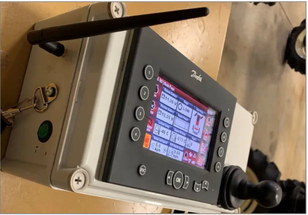
Remote operation was developed using a Danfoss DP600TM display, a Danfoss JS1000 joystick, and Magnetek WIC-2402 Wireless CAN Bridge. These components were mounted in an enclosure with a strap which held the device for comfortable operation (Figure 2.1).

The laptop used a universal serial bus (USB) to CAN bridge for reading and writing messages on Flex-Ro’s CAN bus. The FlexRoRun application programmed using MATLAB app designer, was developed to facilitate high level navigation control. The CAN bridge used was a Kvaser Memorator Pro x2 HS (Kvaser AB, Mölndal, Sweden). A Vector CANcase XL Log (Vector North America Inc. Novi Michigan) was also used during testing.

(35)

Shown in Table 2.1 is the list of primary components which were implemented as part of the control system for the Flex-Ro machine.

Table 2.1: List of control system hardware used on the Flex-Ro machine.

Model Manufacturer Purpose

MC024-110 Danfoss Electronic control unit (24 pin) MC012-110 Danfoss Electronic control unit (12 pin) WIC-2402 Magnetek Wireless radio CAN bridge Victor SPX Vex Robotics Steering motor controller

JS1000 Danfoss Joystick for machine maneuvering DP600TM Danfoss Display for remote operation Memorator Pro 2xHS v2 Kvaser USB to CAN bridge

AG-372 Trimble GPS receiver

O3M151 ifm 3D Smart Sensor, obstacle detector

O3M950 ifm IR illumination unit

2.2.2 CAN Bus J1939 Distributed Control Network

A distributed control network has many advantages. The controllers within the system split the processing of inputs and outputs for each subsystem. A controller of the system, usually with direct operator inputs, sends out machine control messages. For example, the operator commands the machine to slow down and steer to the right using a joystick. The hydrostatic drive controller will receive the message to slow down and adjust the

(36)

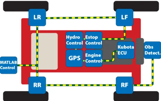
turn right and actuate the wheel angle to the desired operating position. Another benefit of the distributed control network is the ability to add or remove nodes without affecting the rest of the system. The nodes of the Flex-Ro bus can be seen in Figure 2.2.

A CAN bus network connects compatible ECU’s with a twisted pair of wires (Bell, 2002). These wires are used to send data bits across the bus. This data is received by other controllers and processed as commands or machine data. One standard high-level protocol for the formatting of these bits is SAE standard J1939 (Bell, 2002; Marx, 2015). The standard specifies how these data bytes are grouped and sent, called messages. Each message contains identifier bytes and a data payload. The identifier provides information to the ECUs on where the message came from and what it contains. The other ECUs on the bus can choose to process the message if programmed to receive it or ignore it.

Figure 2.2: CAN node layout on the Flex-Ro platform. Dashed wire shows connection via J1939 CAN bus.

(37)

The J1939 standardized communication provides a means to easily record machine data (Marx, 2015; Rohrer, 2017). Many devices have been developed to enable receiving and publishing messages on the CAN bus. A USB to CAN bus bridge allows the computer to send and receive messages in real time. There are many software applications for CAN logging and real-time decoding (Rohrer, 2017). However, programmatically sending CAN messages using a laptop in response to inputs is more limited. MATLAB, LabVIEW, and Visual Studio are a few examples. MATLAB was chosen to design a graphical user interface (GUI) given its ability to utilize existing hardware and the accessibility to useful toolboxes. The MATLAB developed Vehicle Network Toolbox is a suite of functions for sending and receiving messages on the CAN bus. The user can reference a database which MATLAB uses to automatically decode and encode message data. Further, the MATLAB app can be deployed to an executable file so others could install the program and run the Flex-Ro machine.

The messages created for the Flex-Ro platform used J1939 standard and proprietary formats. The source addresses selected for each ECU corresponded to global source addresses defined in the standard. Data to be transmitted used existing SLOT (scaling, limit, offset and transfer) definitions when applicable. Each of the messages were sent as broadcast without specific destination addresses. Priority was assigned based on urgency of the message. For example, the e-stop message received the highest priority to ensure the quickest response time to emergency.

(38)

2.2.3 Human Machine Interface 2.2.3.1 Remote Control Operation

A machine remote-control interface is necessary for basic operation. Navigating from a storage location to field or loading onto trailer requires safe and reliable human control. Indoor automatic guidance for a field machine is impractical due to unpredictable building enviroments and loss of GPS signal for location information. The Flex-Ro wireless remote control must be able to drive the machine, monitor operating variables, change system parameters, and perform an alignment of the steered wheels. The remote uses a display and joystick for intuitive ergonomic control. The right hand is dedicated to controlling the machine travel and steering via the joystick. The left hand is free to adjust parameters on the screen including the brake release, speed range, steering mode, and most importantly the e-stop.

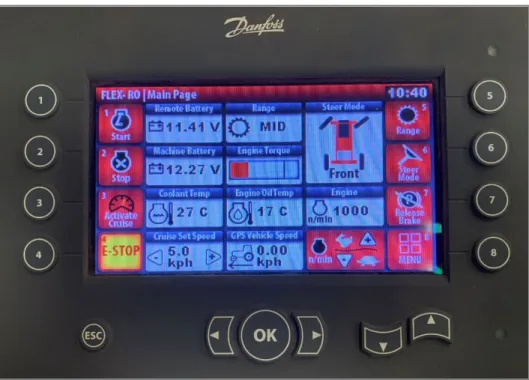
The remote application was programmed using Danfoss PLUS+1 GUIDE software. The main screen of the remote-control interface includes information and controls for normal operation. This main display is shown in Figure 2.3.

(39)

The numbered softkeys were mapped to controls for engine run and start, cruise

activation, e-stop, speed range, steer mode, brake release, and menu access. The machine is programmed to stop when an obstacle is encountered. The operator can override the obstacle detection by pushing and holding the ‘OK’ button. Obstacle detection resumes once the button is released. Engine rotations per minute (rpm) and cruise set speed are adjusted using the arrow key pairs. The current softkey assignment is displayed on the screen as an icon. This includes changing controls, for example, brake release or apply which depends on the current machine state. There are graphics for the current speed range and steering mode. Values displayed on the main screen include remote and machine battery voltage, coolant and engine oil temperatures, cruise set speed, and GPS indicated vehicle speed.

Figure 2.3: Main operating screen of the Flex-Ro remote. Danfoss DP600TM display.

(40)

The second page is the steering calibrate page which is shown in Figure 2.4 (Right). Optical quadrature encoders provide feedback for the steered wheels. The position of the wheel must be calibrated as the encoder only provides a relative pulse count. The count is zeroed at the wheel center position during calibration. The gearing of the steering motor and resolution of the encoder translates to +/- 42,186 counts to +/- 90-degree steering angles. Current absolute wheel position is saved at 2 Hz to non-volatile memory in case the machine is shut-off while the wheels are not at 0 degrees. The steering calibrate page includes controls for activating steering calibrate mode, changing which wheel to

calibrate, and saving new center position. The graphics display which wheel is currently being calibrated. Outside of calibration mode graphically shows the current feedback angle of each wheel. Finally, included on the steering calibration screen is the same e-stop softkey in case of unintended steering or machine motion.

The last screen currently implemented is a diagnostic display, Figure 2.4 (Left). The e-stop button remains and is assigned to the same softkey. The diagnostics screen shows which ECU triggered an active e-stop. The user can then quickly diagnose the root cause of the e-stop flag. Also shown are engine hours, fuel rate, engine oil pressure, compass

(41)

bearing, and estimated fuel level. Two of the softkeys are for resetting the fuel level to either a full or half tank. More modules could be easily added to the diagnostic screen depending on the need of the operator.

The remote-control interface was developed such that individuals with no experience could operate the machine with minimal instruction. Components and information displayed on the screen can be easily changed, added, or deleted depending on the application installed on the machine. The remote is not, however, intended to become a high-level controller. An operator cannot drive to the field and select a navigation path using solely the remote at the time of publishing. Remote operating instructions are included in Appendix B.1.

2.2.3.2 Laptop and MATLAB Control Interface

Autonomous operation of the machine requires processing beyond the capability of a typical microcontroller. The high-level machine controller processes the current machine pose and position and calculates a steering angle. A high-level controller programmed using MATLAB App Designer was developed for Flex-Ro. While not proposed as a long-term solution for machine control, the use of the laptop provided many benefits including the ability to quickly develop and debug programs and implement a graphical user interface. The MATLAB Vehicle Network Toolbox provided the framework needed to communicate with the machine’s J1939 CAN bus controllers. The MATLAB app, called FlexRoRun, was deployed as an executable application. Other users could then install the program without a MATLAB license.

(42)

Operation of the program begins with the initialization of the USB to CAN bridge.

Currently, the tool supports a Vector CANcase XL Log and Kvaser Memorator Pro 2xHS v2. A CAN message database file was created which contained both J1939 standard and custom Flex-Ro messages. Use of the database streamlines the decoding and encoding process of message transmission. The main program execution loop is time triggered at 5Hz. This rate was chosen to match the incoming signal from the GPS and was sufficient for the dynamics of the machine.

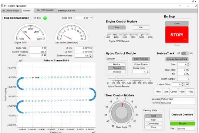
There are several parts to the FlexRoRun main run page as shown in Figure 2.5. Each of the main control systems were divided into modules. Essential engine, hydrostatic drive, steering, and e-stop controls are accessed on the main run page. Keyboard shortcuts were mapped to buttons and sliders, which reduced error prone mouse clicking. The

NebrasTrack (Flex-Ro’s automatic navigation system) controls are also located on the main run page. The module includes a map of the current track and machine’s location, tracking activation, and steering control output for debugging. Lateral shift buttons provide fine and coarse adjustment of tracking location relative to the defined path.

(43)

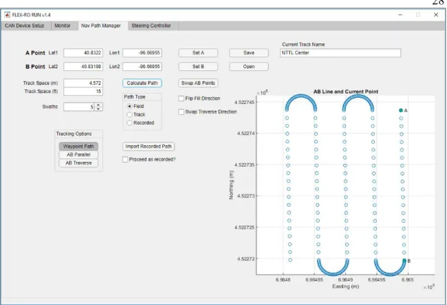
The Navigation Manager page (Figure 2.6) contains track creation controls. There are several ways to import a navigation track. Recording an AB line requires either manual entry of the latitude and longitude coordinates or driving to the A and B points. The user can then generate a field coverage map, assuming a rectangular field. Parameters include track width, and number of swaths. Points are populated based on the recorded AB

points, and a simple constant radius headland turn is calculated. The other tracking modes can also be activated on this page. Modes include waypoint following, AB Parallel

passes, and AB Traverse headland turns.

Figure 2.5: Main application tab for the FlexRoRun application. Developed using MATLAB App Designer.

(44)

The navigation tab includes controls for importing and saving a prerecorded path. Saving a track saves the point array and track metadata, such as track-width, navigation type, and track name. The current track is saved during application shutdown. When the

application is relaunched the last used settings and track are loaded. Basic FlexRoRun operating instructions are included in Appendix B.1.

2.2.4 Low Level Machine Control 2.2.4.1 Engine Control

The engine control ECU receives start and stop commands via a CAN message from the main machine controller (either remote control or FlexRoRun). Those signals are

Figure 2.6: Navigation tab within the FlexRoRun application. Developed using the MATLAB App Designer.

(45)

processed into digital outputs of the run and start pins of the Kubota engine ECU. The engine control ECU translates requested engine rpm into a TSC1 J1939 standard message. The engine control CAN message contents are defined in Table 2.2.

Table 2.2: Engine control message. Start and Length shown as Byte.bit

2.2.4.2 Hydrostatic Drive Control

The hydrostatic drive (hydro) control ECU processes drive command messages into pump control signals. The pump controls machine speed by varying the swash plate angle of the tandem piston pump. Each pump supplies two drive wheels so the swash plate commands must be the same. These commands are either received via remote joystick or from the high-level controller. Before the machine can be moved, a brake release signal must be received. Once the command is processed, the control-cut-off valve is activated which supplies pressure to the wheel brakes. The brakes are in normally ON position with spring pressure. Direction and magnitude commands are included in the hydro control CAN message described in Table 2.3. Ramp up and down parameters are programmed into the controller for smooth acceleration and to avoid damage to the

Message Description: Engine control data from main machine controller. ID: 0x10FF4427

Start: Length: Description:

0.0 0.2 Engine run enumeration 0.2 0.2 Engine start enumeration 1.0 2.0 Engine RPM request

(46)

pump. The deceleration was tuned so the machine slows rapidly and without tire skid. A cruise control function is also supported which controls the swash plate angle using a closed loop between requested and actual machine speed.

The hydro-controller also processes the machine’s response to detected obstacles. The hydro controller manages vehicle speeds, so if an obstacle is detected, the controller can react quickly. The function of the obstacle detection algorithm is covered more in depth in Section 2.2.8.

Table 2.3: Hydrostatic drive pump control message. Start and Length shown as Byte.bit

Message Description: Hydro. control data from main machine controller. ID: 0x4FF4127

0.0 0.2 Direction enumeration 0.2 0.2 Brake release enumeration 0.4 0.2 Cruise control enumeration 0.6 0.3 Obstacle override enumeration 1.0 2.0 Drive magnitude

(47)

2.2.4.3 Steering Control

There is a steering control ECU located at each wheel. A CAN message sends a

commanded center steering angle as well as the current steering mode enumeration. Each ECU processes this message using a PLUS+1 GUIDE Ackermann steering block

(Appendix D.2). This block calculates the wheel angle based on the mode and centerline command. There are four programmed steering modes; front, rear, coordinated, and crab. The centerline commanded angle and steering mode are included in one of the steering messages described in

Table 2.4. A closed loop PI controller commands a motor driver via PWM (pulse width modulation) signal to turn the wheel. Digital encoder pulses are counted to determine the wheel’s current angle. There are +/- 42,186 pulses to turn +/- 90°. Direction of turn is determined by the sign of the phase offset between A and B encoder channels. The controller periodically saves the absolute wheel position in case of machine power down.

(48)

Table 2.4: Steering control messages. Start and Length shown as Byte.bit

Each of the four wheels steers independently of the others. Ackermann’s steering angles require the inner and outer wheels to steer to different angles based on a centerline commanded angle. In this system, the wheels may arrive at their individual commanded angle at separate times. This is especially apparent at very sharp steering angles when the inner wheel angle turns to 90-degrees and the corresponding outer wheel angle is near 60-degrees. Synchronization was implemented to slow the speed of the wheel that has a smaller delta to the next commanded steer angle. Tuning adjusted the proportion gain on the delta until the wheels arrived at extreme steering angles simultaneously.

Message Description: Steering command information. ID: 0x8FF4327

0.0 2.0 Centerline commanded steer angle 2.0 0.2 Steer mode enumeration

Message Description: Steering calibration commands. ID: 0x1CFF4527

0.0 0.2 Calibration mode enable 0.2 0.2 Active calibration wheel

(49)

Each steering ECU also monitors a physical e-stop switch. When the switch continuity is broken, an e-stop flag is immediately sent across the CAN bus with the highest priority. The flag remains until the e-stop switch is reset, and control is resumed when the user resets the machine with the remote or FlexRoRun software.

2.2.4.4 Emergency Stop Network. Start and Length shown as Byte.bit

Each of the controllers sends a status message at 10 Hz. The main machine controller (remote control or FlexRoRun) processes the status messages from all the machine controllers to check for e-stop flags. If the main controller does not receive a message from an ECU after 2 seconds, an emergency flag is set. After a flag is set, all controllers must send a reset signal to ensure the machine is ready to return to service. A heartbeat signal within each message ensures that the controller is properly functioning and is on the bus each time a new message is sent. The contents of the status CAN message are outlined in Table 2.5.

Table 2.5: Example status message. Start and Length shown as Byte.bit

Message Description: Status message from hydrostatic drive controller. ID: 0x0FF572E

Start: Length: Description: 0.0 1.0 Heartbeat (0 – 255)

(50)

2.2.5 Navigation Error Calculation

The implementation of a straight-line tracking algorithm is the first step for automatic navigation. The operating environment for the Flex-Ro machine is row crop fields. Successful navigation down the rows without crop damage is of highest importance for the machine. There has been a significant amount of research in the implementation of various controller algorithms for automatic steering (Bell, 1999; Boyali et al., 2018; Godoy et al., 2012; O’Connor, 1997; Troyer, 2017). Kinetic based control while simple and effective, lacks robustness during higher speeds. Dynamic control algorithms require more development time, as well as a higher number of sensor inputs and computational power. The navigation controller for Flex-Ro was first developed using a kinetic model. The first step in determining an output steering angle was calculating the lateral

(perpendicular) error from the desired tracking line. This desired tracking line was defined by two points (A and B) recorded in latitude and longitude coordinates.

Conversion from latitude and longitude degrees to Universal Transverse Mercator (UTM) coordinates in meters enables a direct calculation of lateral error. Conventionally, the easting direction is along the UTM x axis while the northing direction is along the UTM y axis. The calculation of the lateral error uses three points, A, B and current position, C. The cross product by the vector 𝐵𝐵𝐵𝐵��⃗, and the vector 𝐵𝐵𝐵𝐵��⃗, gives the area of the

parallelogram (shaded in Figure 2.7) formed by the two vectors. A parallelogram must have the same area as a rectangle (orthogonal sides) with the same perpendicular distance between parallel lines. Thus, the area divided by length from B to A ( �𝐵𝐵𝐵𝐵��⃗� ) results in

(51)

the perpendicular distance L from the line 𝐵𝐵𝐵𝐵 to point C. This calculation is valid at any point along the line 𝐵𝐵𝐵𝐵 (navigation line).

The sign of the lateral error has not been applied at this point. The sign convention is to remain the same regardless of machine orientation. The navigation control system will manage the controller response based on if the machine is traveling in forward or reverse. The calculation of the sign depends on the difference in slopes between the navigation line machine’s current point. The convention was developed based on point A shown in Figure 2.7. It should be noted that the UTM coordinates will always be positive values, alleviating potential complications. Only the sign of the slope difference is applied to the lateral error. The MATLAB script for calculating lateral error is attached in Appendix D.1 for reference.

(52)

Equation 2.1: Perpendicular offset from navigation line calculated from three points, where A and B define the navigation line

𝑙𝑙𝑙𝑙𝑙𝑙𝑙𝑙𝑙𝑙𝑙𝑙𝑙𝑙𝑙𝑙 = �𝐵𝐵𝐵𝐵��⃗_{�𝐵𝐵𝐵𝐵}_{��⃗�} × 𝐵𝐵𝐵𝐵��⃗�

Equation 2.2: Applying the sign of lateral error based on the line (AB) and current points.

𝑙𝑙𝑙𝑙𝑙𝑙𝑙𝑙𝑙𝑙𝑙𝑙𝑙𝑙𝑙𝑙= 𝑙𝑙𝑙𝑙𝑙𝑙𝑙𝑙𝑙𝑙𝑙𝑙𝑙𝑙𝑙𝑙 ∗ 𝑠𝑠𝑠𝑠𝑠𝑠𝑠𝑠 ��𝐵𝐵_𝐵𝐵𝑦𝑦− 𝐵𝐵𝑦𝑦

𝑥𝑥− 𝐵𝐵𝑥𝑥� − �

𝐵𝐵𝑦𝑦− 𝐵𝐵𝑦𝑦

𝐵𝐵𝑥𝑥− 𝐵𝐵𝑥𝑥�� 2.2.5.1 Heading Error Calculation

It is important to know the current machine heading for navigation control. The Trimble Ag-372 GPS publishes heading information along with the GPS indicated speed and location on the CAN bus. The compass heading convention defines North to be 0° with positive clockwise rotation (i.e. driving straight east is a 90° heading). A limitation of the GPS unit was that the heading couldn’t accurately be determined until the machine was in motion. However, this would only be a factor for a very short period as the vehicle

initialized motion. More accurate methods of determining heading, including the use of two GPS units, will be considered for future development.

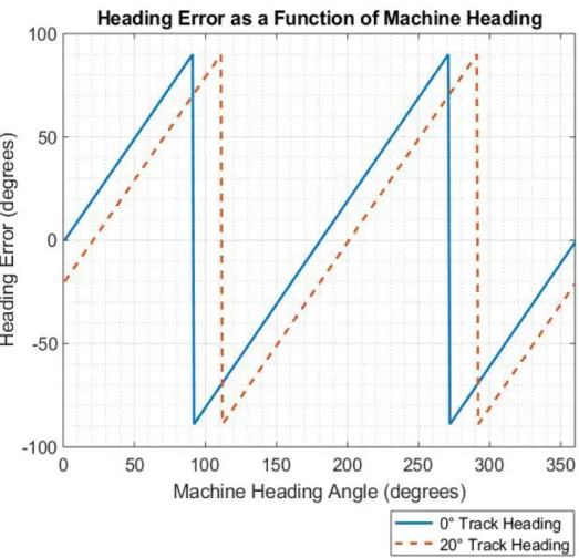
The Flex-Ro machine was to navigate down a path in either direction. The heading error was defined as the current machine heading minus the track heading. The track heading was defined as the angle from due north clockwise to the line formed by A and B. Also, the A and B points can be swapped with no effect. In other words, if the machine heading is 180° off the track heading, there should be no heading error. The result of such

(53)

following is 0° (straight north) and 20° clockwise from north as examples.

The track heading was calculated using the ‘legs’ MATLAB mapping toolbox function. The two navigation points in latitude and longitude are aruguments and provide an output in degrees in the standard compass coordinate system, directly comparable to the GPS heading output.

(54)

2.2.6 Waypoint Navigation

Waypoint navigation is defined as following a path which is defined by a matrix of points. The machine navigates from point to point in the sequence defined by the path matrix. The path can be any shape, but in its most basic form a straight line is drawn between points. The curvature of the path can be calculated by using the next three points ahead. Waypoint following is used for navigation of paths other than straight A and B point parallel tracking.

MATLAB provides a kinematic based function for calculating a steering angle based on pose, heading error, and velocity. This equation is based on research completed at Stanford University, by Hoffmann et. al (2007) and Paden et. al (2016). The control equation was originally used on a car named Stanley which competed in the DARPA Grand Challenge 2005. The base function uses a pure pursuit type strategy without accounting for curvature of the path.

Flex-Ro uses the factors of the Stanley Lateral Controller slightly different than it was designed. Arguments into the equation are reference pose and current pose. This method reflects the pure pursuit nature of the controller. Flex-Ro required a stable line following algorithm with GPS coordinates. As the lateral and heading errors were already

calculated, the current pose (machine origin) was set to zero. As a result, the distance to point in the x direction (longitudinal) became a tunable factor, and the y distance (lateral) was set to be the lateral error as shown in Figure 2.9. The heading error was set as the reference heading.

(55)

The other tunable factor was the position gain. The position gain controlled how

aggressively the machine responded to lateral error. Increasing the gain would result in a system with a quicker response and less steady state error, but also caused instability as speed increased.

Waypoint navigation included more than the straight AB lines mentioned above. First, it was desired that the machine could start a path at any point and traverse in either

direction. The cycle time also had to be fast enough for smooth navigation without lag. The machine position and heading would then have to determine what points in the path would be used for navigation. A navigation path selection algorithm selected the next three points that were in front of the machine, and within a maximum lateral error. The waypoint paths were stored in a matrix of UTM x and y coordinate locations. When navigating, during each program cycle, the matrix of points is transformed into the machine coordinate system using the current heading of the machine. (The transformed

(56)

points are indexed to their original UTM coordinates to retain accuracy due to error in the heading data.) Then the points can be sorted and filtered. The negative x points (behind the machine) are eliminated. Then programmatically, the points in front of the machine are checked to ensure they are within the current swath. The first two points (in UTM coordinates) are then used for the lateral and heading error calculation. The first three points (in machine coordinates) are used to calculate the curvature of the upcoming path. The curvature is used as an added factor to the pure pursuit type algorithm. The current path curvature is calculated by using a custom MATLAB function (Mjaavatten, 2018). The curvature of the upcoming path is used to bias the steering angle based on the geometry of the machine. This function outputs the vector which points to the center of the circle defined by the three points. The sign of the y coordinate tells whether the path is curving left or right, and the direction of the required steering angle as a result. The bias of the steering angle helps correct for upcoming curvature in the path but does not provide information on whether the machine is inside or outside the curve. Short linear segments are used to calculate the lateral and heading error information. The steering angle from the Stanley controller is then added to the steer bias and then sent via centerline commanded angle message to the steering ECUs.

2.2.6.1 Field Path Generation

The basic operating environments for the Flex-Ro machine are research plots with straight rows. There are open headlands with plenty of clearance for turning at the end of the rows. A basic tool for generating these types of field paths was developed for quick

(57)

processing once the machine was on-site. One advantage would be to navigate fields without access to as planted navigation data. The A and B points were set by positioning the machine in a set of rows at each end of the field. Parameters such as the track width, fill direction, and number of swaths were entered and then a path is calculated. If the as planted navigation track data was available, the latitude and longitude coordinates of the A and B points could be entered directly to calculate the field coverage swaths.

2.2.6.2 Recorded Path Import

Paths which are driven in semi-controlled environments are well suited for autonomous navigation using the Flex-Ro’s waypoint navigation. The FlexRoRun application

processes data which contains navigation performance and machine position information. A record button on the FlexRoRun main page toggles the saving of this data to a log file accessible by the program. If the user wants to record a path, a log is taken while the user manually drives the machine down a path. Then, within the NavManager tab, this log is loaded and processed into a waypoint path. The path can then be followed as recorded (following the same direction) or in either direction. Lateral offsets can also be added to compensate for multiple swaths of the same recorded path.

2.2.7 Headland Turn Strategies

A headland turn is the maneuvering a machine from one working pass to the next. There are multiple ways to complete a headland turn. The independent four-wheel steer

capability of the Flex-Ro enables four different steering strategies. Changing the instantaneous center of rotation (ICR) is possible to maximize turn efficiency. Crab

(58)

steering allows for sideways travel. Thus, a headland ‘turn’ can be completed without changing machine direction. There are advantages and disadvantages to both types of turn strategies. The scope of this thesis was to compare the traditional front wheel steering method with the traverse type (Figure 2.10).

2.2.7.1 Conventional Radius Turn

The conventional method of steering consists of a fixed rear axle and Ackermann’s angles for the front wheels. The turn begins once the vehicle has fully entered the headland. There are multiple paths the machine can follow when completing a front wheel turn. The simplest is a semicircle tangent to the crop swath passes or U turn. This path can be easily generated using the AB points of the path, and the desired track width. The density of points on the arc directly affects the accuracy of the machine path

following using the Flex-Ro waypoint algorithm.

Figure 2.10: Left: Conventional front wheel steer headland turn. Right: Traverse headland navigation method.

(59)

2.2.7.2 Headland Traverse

The headland traverse turn is activated once the machine fully enters the headland. This area is currently defined as the zone outside the crop rows and perpendicular to

navigation segment AB. The machine stops and waits until the wheels turn to 90°. The machine then slowly travels until the lateral error to the next swath is less than 10 cm. The machine then stops, waits until the wheels have returned to their normal orientation, and proceeds down the next path.

2.2.8 Obstacle Detection

Traditional machinery operators function as obstacle detectors. Autonomous operation requires either a completely controlled area of operation (no possibility of obstacles) or sensors which can warn of upcoming collisions. The motivation for installing the obstacle detection system is primarily for operator and bystander safety. Damage to the machine and its operating environment were also concerns which could be mitigated with the implementation of an obstacle detector. The objectives for the obstacle detection system are as follows:

1. Implement an obstacle detection sensor into the CAN based vehicle control architecture of Flex-Ro.

2. Stop Flex-Ro automatically within 1-2m of a pedestrian sized object at typical field operating speeds.

(60)

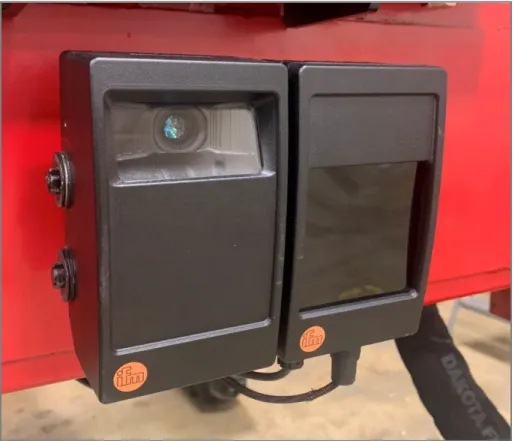
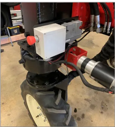
It was important to implement obstacle detector solutions for Flex-Ro which would utilize the existing J1939 CAN bus network. The O3M 151 3D Smart Sensor produced by ifm (ifm efector, inc. Malvern, PA) used J1939 messages to transmit processed object information and is seen in Figure 2.11.

This sensor uses an IR (infrared) pixel array to calculate the time of flight and resulting distance to object. The pixel matrix consists of 64 (horizontal) x 16 (vertical) IR dots, over an aperture size of 70° (horizontal) x 23° (vertical). The range is advertised to be 35 meters. However, at that distance, one IR pixel covers 77 x 91 cm. As a result, the object would have to be very large (e.g. dump truck) for reliable detection. The relatively slow

Figure 2.11: ifm O3M 151 3D Smart Sensor installed on the front of the Flex-Ro platform.