Received July 31, 2020, accepted September 8, 2020, date of publication September 18, 2020, date of current version October 1, 2020. Digital Object Identifier 10.1109/ACCESS.2020.3025196
GANs-Based Data Augmentation for
Citrus Disease Severity Detection
Using Deep Learning
QINGMAO ZENG1, XINHUI MA 2, BAOPING CHENG3, ERXUN ZHOU4,
AND WEI PANG5
1Department of Mathematics, College of Mathematics and Informatics, South China Agricultural University, Guangzhou 510642, China 2Department of Computer Science and Technology, University of Hull, Hull HU6 7RX, U.K.
3Guangdong Provincial Key Laboratory of High Technology for Plant Protection, Guangdong Academy of Agricultural Sciences, Guangzhou 510640, China 4Guangdong Province Key Laboratory of Microbial Signals and Disease Control, South China Agricultural University, Guangzhou 510642, China 5School of Mathematical and Computer Sciences, Heriot-Watt University, Edinburgh EH14 4AS, U.K.
Corresponding author: Xinhui Ma ([email protected])
This work was supported in part by the China Scholarship Council under Grant 201708440539, in part by the Guangdong’s Modern Industrial Technology System Fund for Common Key Technologies Development (2019), and in part by the Guangdong Modern Agricultural Technology System Fund under Grant 2019KJ113 and Grant 2019KJ116.
ABSTRACT Recently, many Deep Learning models have been employed to classify different kinds of plant diseases, but very little work has been done for disease severity detection. However, it is more important to master the severities of plant diseases accurately and timely, as it helps to make effective decisions to protect the plants from being further infected and reduce financial loss. In this paper, based on the Huanglongbing (HLB)-infected leaf images obtained fromPlantVillageandcrowdAI, we created a dataset with 5,406 citrus leaf images infected by HLB. Then six different kinds of popular models were trained to perform the severity detection of citrus HLB with the goal to find which types of models are more suitable to detect HLB severity with the same training circumstance. The experimental results show that the Inception_v3 model with epochs=60 can achieve higher accuracy than that of other models for severity detection with an accuracy of 74.38% due to its highly computational efficiency and small number of parameters. Additionally, aiming for evaluating whether GANs-based data augmentation can contribute to improve the model learning performance, we adopted DCGANs (Deep Convolutional Generative Adversarial Networks) to augment the original training dataset up to two times itself. Finally, a new training dataset with 14,056 leaf images composed by the original training images and the augmented ones were used to train the Inception_v3 model. As a result, we achieved an accuracy of 92.60%, about 20% higher than that of the Inception_v3 model trained by the original training dataset, which suggested that the GANs-based data augmentation is very useful to improve the model learning performance.
INDEX TERMS Citrus Huanglongbing, data augmentation, deep learning, generative adversarial networks, plant disease severity.
I. INTRODUCTION
In recent years, Deep Learning models are widely employed in plant disease classification and identification prob-lems [1]–[7]. However, very little work has been done for disease severity detection.
From the practical point of view, reliable, accurate and timely detection of plant disease severity is more impor-The associate editor coordinating the review of this manuscript and approving it for publication was Quan Zou .
tant for farmers comparing to disease classification, as dis-ease severity detection is helpful to assist them to make effective decisions to protect the plants from being further infected, reduce financial loss [8], and it is beneficial to predict yield loss, monitor and forecast epidemics, assess crop germplasm for disease resistance, and better understand basic biological processes such as coevolution [9]. On the contrary, inaccurate and/or imprecise disease assessments might lead to faulty decisions or probably result in severer problems.
Fortunately, some researchers have noticed the related work on the detection of plant disease severity [8]–[11], but most of them encountered the problem of time consuming hand-crafted feature extraction, which heavily depends on a series of image-processing technologies. Although some efforts have been made to address the above-mentioned problem [11], there are still many research gaps that need to be filled. For example, the types of Deep Learning mod-els used to assess the performance are very limited without considering some new kinds of models presented in recent years. In addition, in order to train a Deep Learning model, the variability and scale of the datasets should be considered in advance.
Citrus Huanglongbing (HLB) is also known as Citrus Greening disease because the infected fruits tend to turn green after ripening [12]. HLB is one of the most destructive diseases of citrus worldwide, which is called citrus ‘‘cancer’’ by some people due to its incurability. The most characteristic symptom of HLB-infected citruses is that their leaves have a blotchy mottled appearance [13] as shown in Fig. 1.
FIGURE 1. Blotchy mottle, the HLB early symptoms [14].
In practical conditions, in order to avoid or decrease the losses caused by HLB, different levels of HLB severities have their corresponding measures. Generally speaking, if the citruses are lightly infected, namely infected in the early stage, the orchard should be conducted molecular detection at regular intervals to find and control the disease as early as possible. Moreover, in the case of being infected by the exter-nal bacteria, we should take care of the prevention and control of a psyllidvector known as Diaphorina citri, which will transmits a phloem-limited bacteriumCandidatus Liberibac-ter asiaticus(Las), the causal agent for HLB. When the cit-ruses are in the moderately infected stages, we should enforce the cultivating management to slow down the process of citrus recession and keep yield from decreasing too fast. At the same time, it is also necessary to be careful of preventing and controlling the citruspsyllidto avoid the HLB-infected citrus further infecting other citruses. If we find that the citruses lie in severely infected stages, we have no choice but to remove the trees. In a word, it is very important for the citrus farmers
and growers to learn the severity level of citrus HLB at their early convenience to make timely decisions.
Sweet oranges are one type of citruses and very popular all over the world. In this work, we create a dataset including the HLB-infected leaves of sweet oranges in three different sever-ity stages, namely Early Stage, Moderate Stage, and Severely Infected Stage. One of our goals is to assess the performance of six different kinds of popular Deep Leaning models to find which one is the most suitable to detect the HLB severity level, hoping to provide a constructive advice for agricultural growers or producers. In addition, in order to increase the size of the training dataset, we employ Deep Convolutional Gen-erative Adversarial Networks (DCGANs) [15] to augment the original training dataset. It was prepared for another goal of our work, namely to investigate whether the augmented data are helpful to improve the learning performance of the selected suitable model.
The rest of the paper is arranged as follows: Section II mainly describes how to create our datasets for training and testing as well as how to label the citrus leaf images. Then some training techniques, the main methods and steps on how to train and test Deep Learning models are presented in Section III. Section IV presents our experimental results and further discussions. Finally, Section V concludes our paper with conclusions and future work. Fig. 2 gives an outline of our research work.
FIGURE 2. The outline of our research work.
II. MATERIALS
A. DATASET FOR TRAINING AND TESTING
For training a Deep Learning model to be an accurate clas-sifier, an image dataset with proper and balancing sizes of variable types of samples is always needed [16]. Generally speaking, when we have relatively balancing sizes of different classes, the larger the dataset size is the more accurate deep
learning model we can obtain. Hence, at least a few hundreds of images for each class are required for training a Deep Learning model [3].
Fortunately, there are more and more image resources publicly available on the internet, which makes it conve-nient for researchers to make use of them to facilitate the training. In this research, our data are mainly collected from PlantVillage [2], [17] and crowdAI [18], which include 5,507 citrus leaf images. However, 101 images were dropped by us because they are not typical HLB symptoms or probably caused by other diseases. The rest are 5,406 images that are all typically HLB-infected citrus leaf images, which were split into a train dataset with 4,325 images and a test dataset with 1,081 images.
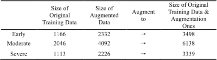
Furthermore, in order to test whether the technique of GANs-based data augmentation is helpful to improve the model performance, we adopted DCGANs to augment the size of the training dataset to three times that of the original training dataset. Finally, we create a new training dataset with 4, 325×3=12,975 citrus leaf images in total, including the original training data (4,325 images) and its augmented data (8,650 images).
B. IMAGE LABELLING
Almost all of the images downloaded from the websites are infected by HLB without distinguishing their infected sever-ities. Hence, we should relabel all of the HLB-infected leaf images into different severity stages before using them to train and test a Deep Learning model.
Above all, a labeling standard is created according to our domain specific knowledge and classification experience. Considering that a blotchy mottled appearance is the most characteristic symptom of HLB, we measure the severity of HLB from three aspects, including
• the ratio of yellowing area to leaf area • the leaf vein occupied by the yellowing part • the leaf’s yellowing level
The detailed measuring method is shown in Table 1. TABLE 1. The method to measure the severity of HLB.
After giving the scores from the above three aspects, we sum them to get the severity of HLB. The following is our labeling standard:
• If the total score is from 1 to 3 points, we classify the HLB into Mildly Infected Stage (Early Stage).
• If the total score is from 4 to 6 points, we classify the HLB into Moderately Infected Stage.
• If the total score is more than 7 points, we classify the HLB into Severely Infected Stage
Fig. 3 shows the samples in three different stages for the original citrus leaf dataset.
FIGURE 3. Citrus leaves in different stages.
According to the methods to measure the severity of HLB, three experts were invited to manually classify the HLB-infected leaf images. Each leaf image will get three scores from three experts. Then the average scores will be calculated. It is based on the average scores that we classified the HLB-infected leaf images into different severity levels.
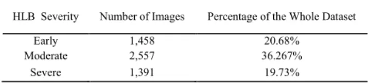
Finally, we create a dataset with 5,406 original images including 1,458 in Early Infected Stage, 2,557 in Moder-ately Infected Stage, and 1,391 in Severely Infected Stage, as shown in Table 2.
TABLE 2.The basic information for the Citrus leaf image dataset.
III. METHODS
A. DEEP LEARNING MODELS AND TRAINING STRATEGY
In [2], Brahimi et al. trained six Deep Learning models, namely AlexNet, DenseNet-169, Inception v3, ResNet-34, SqueezeNet-1.1, and VGG13, for plant disease classification experiments, where three different training strategies were applied to each model. The first training strategy is called Shallow Strategy, which is a transfer learning approach. The Shallow Strategy fine-tunes only at the fully connected layers and the rest layers act as feature extractors. The second training strategy is calledDeep Strategy, which is also a trans-fer learning strategy but fine-tunes parameters of all layers. Both of the strategies aim to make Deep Learning models learn more specific features for plant disease classification from the pre-trained models. The third training strategy is calledFrom-Scratch Strategybecause it starts from random configured weights. Their experimental results show that all six models with the training strategy of Deep Strategy are better than the other training strategies, from the point of classification accuracies of plant diseases.
In our work, our main task is to study how to detect the severities of citrus HLB, that is to say, distinguish three subclasses from the class of HLB, which needs the models to extract finer features from the citrus leaf images than those
in [2]. In order to find which Deep Learning model and how many epochs are more suitable to detect citrus disease sever-ity, all the six Deep Learning models are chosen to train and test with the same learning strategy (Deep Strategy) because, comparatively speaking, Deep Strategy is better than Shallow Strategy and From-scratch Strategy based on the study of [2]. 1) AlexNet
One of the main breakthroughs in deep convolutional networks was the development of AlexNet [19], which won the ImageNet Large Scale Visual Recognition Chal-lenge (ILSVRC) in 2012, one of the most difficult chalChal-lenges for image detection and classification. The basic layout of AlexNet architecture is as follows [20]:
• The first convolution layer fulfils convolution and max pooling with Local Response Normalization (LRN). • The second layer performs the same operations as the
first one.
• The third, fourth and fifth convolutional layers employ 3 × 3 filters with 384, 384 and 256 feature maps respectively
• The sixth and seventh layers are both fully connected layers with dropout.
• The last layer is a Soft-max layer.
2) VGG
In order to investigate the effect of the convolutional network depth on its accuracy in the large-scale image recognition setting, Karen Simonyan and Andrew Zisserman from Visual Geometry Group, University of Oxford, proposed VGG mod-els, which have won the ImageNet Challenge 2014 in the localisation and classification tracks [21]. The basic architec-ture of a VGG model is as follows [20]:
• The first and second layers are convolutional layers with ReLU as activation functions.
• The third layer is a single max pooling layer
• From the fourth layer on, the structure from first to third layers are repeated. The repeating times depend on the network’s depth.
• After several repeating convolutional and max pooling layers, there are followed three fully connected layers with ReLU as activation functions.
• A Soft-max layer for classification is in the model’s last layer.
Four VGG models, VGG-11, VGG-13, VGG-16 and VGG-19 were proposed in [21]. These models had 11, 13, 16 and 19 layers, respectively.
3) ResNet
Deep Residual Networks, ResNet won the 1st place in the ILSVRC & COCO 2015 competition. In order to ease the training of deeper networks, Heet al. proposed ResNet [22]. ResNet has been developed with some different numbers of layers. For example, ResNet34 is made up of 33 convolution layers with 1 fully connected layer at the network’s last
layer. Mathematical formulation of ResNet is expressed in the following equations [22], [23]:
g(xi)=f(xi)+xi (1)
f(xi)=g(xi)−xi (2) In (1), f(xi) is a transformed signal, whereas xi is the original input. The original input xi is added to f(xi) through bypass pathways. In (2),g(xi)−xiperforms residual learning [23]. ResNet introduced shortcut connections within layers to enable cross-layer connectivity but these gates are data independent and parameter free, so it makes ResNet have lower computational complexity than VGG even with increased depth.
4) INCEPTION V3
Aiming to explore ways to scale up networks but utilize the added computation as efficiently as possible, Christian Szegedyet al. presented Inception v3, which factorizes con-volutions with large filter size into smaller concon-volutions and spatially factorizes into asymmetric convolutions as well as makes use of auxiliary classifiers. The Inception v3 is an updated version of GoogleNet [24]. Inception v3 was named after the inception module, which uses parallel 1×1, 3×3, and 5×5 convolutions along with a max-pooling layer in parallel, hence enabling it to capture a variety of features in parallel [5]. There are 42 layers in Inception v3, but the computation cost is only 2.5 times higher than that of 22-layer GoogLeNet.
Actually, the advantages of Inception v3 mainly owe to its four design principles. The first principle is to avoid represen-tational bottlenecks in the feed-forward network. The second principle is to use higher dimensional representations to facil-itate local processing within the network. The third principle is that more features can be disentangled by increasing the activations per tile in a convolutional network, and spatial aggregation on lower dimensional embedding will lead to not much or no loss in representational power. The fourth princi-ple is to balance the width and depth of the network. Based on these principles, inception v3 can get high performance. A more detailed overview of the design principles performed to construct the Inception_v3 model from GoogleNet can be found in [5], [6], [24].
5) SqueezeNet
SqueezeNet’s overarching objective is to identify deep con-volution neural networks that have few parameters while conserving good performance. In order to obtain this, the fol-lowing strategies are employed [25]:
• 3×3 filters are replaced by 1×1 filters.
• the number of input channels is reduced to 3×3 filters. • Downsample late in the network to make large activation
maps of convolution layers.
Furthermore, the Fire module is defined, which is com-posed of a squeeze convolution layer, feeding into an expand layer with a mix of 1×1 and 3×3 convolution filters.
Compared to AlexNet, SqueezeNet can achieve the same accuracy level on ImageNet with 50x fewer parameters and 510 x smaller than AlexNet [25].
6) DenseNet
Inspire by the idea that CNNs can be trained to substan-tially deeper, more accurate, and efficient if their connections between layers close to the input and those close to the output is shorter, Huanget al.[26] presented Densely Con-nected Convolutional Network, namely DenseNet, which is composed of densely connected CNN layers, and, in a dense block, each layer’s outputs are connected with all subsequent layers. For each layer, the feature-maps of all preceding layers are used as inputs, and its own feature-maps are used as inputs into all successor layers. Therefore, there are L(L +1)/2 direct connections for a convolutional network with layers. The detailed structures of different DenseNets can be found in [26].
B. IMAGE PRE-PROCESSING
1) USE OF TRAINING DATA
Above all, the original dataset was divided into training and testing datasets. The training dataset includes 80% of the orig-inal dataset, and the rest 20% is included in the testing dataset. In neural network applications, Ferentinos thinks that the 80/20 splitting ratio of training/testing datasets is generally applied, and other similar splitting ratios such as 70/30 should have little impact on the developed model’s performance [3]. Therefore, we randomly choose 4,325 images and use them to train the Deep Learning models while the rest 1,081 images are reserved for testing the model’s performance in distin-guishing the plant disease severities from new, previously ‘‘unseen’’ images.
The batch size is a hype-parameter which determines the number of samples to work through before updating the parameters in a model. According to the batch size, there are three ways to use the training data [27].
• The first one is Batch Gradient Descent, in which the batch size is equal to the size of training set. The advantage ofBatch Gradient Descentis that it can get more accurate concentrating direction to find the optimal point. Of course it also needs huge computer memory and a lot of time.
• The second one isStochastic Gradient Descent, on the contrary, in which the batch size is equal to 1. It means the internal model parameters will update each time for each sample. Apparently, it needs very little memory and is very fast. However, it is easy to make the algorithm divergent.
• The third one is known asMini-Batch Gradient Descent, in which the batch size is between 1 and the size of training set. Therefore, it possesses the advantages of both Batch Gradient Descent and Stochastic Gradient Descent.
Therefore, in our experiments, we choose the third way to train the models. In both training and testing datasets, there are three classes, namely Early, Moderate and Severe respec-tively. As depicted in [28], [29], the batch size=32 take a great advantage of the speed-up of matrix-matrix products over matrix-vector products. Therefore, we set batch size=
32 and Mini-Batch size=16, which means 32×16 = 512 images will be randomly selected from the training dataset as input of the models for each update of network parameters. Furthermore, if the size of dataset is not divisible by the batch size, then the last batch will be smaller, and we will drop the last incomplete batch in our work.
2) IMAGE CROPPING
In order to make the images suitable for the input of the Deep Learning models, we should randomly crop all the images in the experiment to be 224× 224 for AlexNet, SqueezeNet, VGG, DenseNet and ResNet, and 299×299 for Inception as well. In the process of cropping and resizing, we chose the bilinear interpolation, which can reduce the stepped effect created by the nearest neighbor approach and make the images look smoother.
3) TRANSFORMING AND NORMALIZING IMAGES
Before using the images to train Deep Learning models, we should transform images into tensors. Then in order to speed up the training process, we normalize a tensor image with mean and standard deviation. For a color image, there are usually three channels. Given means of three channels areM1,M2,M3and standard deviations areS1,S2,S3 respec-tively. Then we have
Normalizing Channeli=
Original Channeli−Mi
Si ,
i=1,2,3 (3)
C. GANs-BASED DATA AUGMENTATION
1) GANs
Generative Adversarial Networks (GANs) are presented by Ian J. Goodfellowet al.in 2014 [31], [32]. GANs train two models at the same time. One is a generative model called Generator. The other is a discriminative model called Dis-criminator. In the course of training, Generator is employed to capture the distribution of the original data and contin-ually generates new samples with the approximate distri-bution of the original dataset. On the contrary, Discrimi-nator is used to detect whether a sample is from the orig-inal dataset or generated by Generator. The training will be ended when the Generator can generate the high-copy samples of the original data which Discriminator can always properly distinguish the generated and original sample at 50% confidence.
From the description of GANs above, we can see that GANs are employed to instruct a Deep Learning model to obtain the distribution of the original data. Therefore, we can produce new data from the approximate
distribu-tion as the original dataset [32]. Based on this idea, the GANs can be used to augment training datasets by generating new data.
Recently, after the basic GANs was proposed, GANs have been attracting many researchers in different fields, and many different version of GANs have been developed, such as ACGANs [33], BEGANs [34], BicycleGANs [35], DCGANs [15] and so on [36].
2) DCGANs DATA AUGMENTATION
In practical application, GANs are known to be unsta-ble to train, often resulting in generators that produce nonsensical outputs [15]. As a direct extension of the GANs discussed above, DCGANs were firstly presented by Radford et al. [15], [32]. In DCGANs, the Discriminator consists of stride convolutional layers, batch norm layers and LeakyReLU activations, while the Generator is made up of convolutional-transpose layers, batch norm layers and ReLU activations. Owing to the architectural topology of DCGANs, they are stable to train in most setting. Therefore, in order to test whether the augmented data can improve the model performance, we will use DCGANs to augment the training dataset to three times the size of the original one. Then the original training images and augmented ones are used to create a new training dataset. Table 3 gives the specific augmented information.
TABLE 3. The specific augmentation size of different classes.
D. TRAINING AND TESTING MODEL TO FIND THE BEST MODEL
1) SOFTWARE AND HARDWARE FOR IMPLEMENTATION In this work, we employed PyTorch, an optimized tensor library for deep learning using GPUs and CPUs [37], to train models and test their performance.
Our code is largely based on the codes provided by Arsenic [38]. All experiments in this research were performed on the High Performance Computer of the University of Hull named as Viper. There are four general use GPU nodes named GPU01∼GPU04 on Viper, respectively. Each of these nodes have four NVIDIA K40M GPGPU (or sometimes referred to as APU) in them; so a total of 16 units. Furthermore, there is also a GPU node named GPU05, which has two Tesla P100 cards with 16GB of memory. We can see the specifi-cation of GPU on Viper in Table 4. These are connected via PCI-e to Intel 28 core Broadwell processor with 128 GB.
In order to make the experimental results preserve the comparability, all our experiments are uniformly performed
TABLE 4.The specification of GPUs on Viper.
on the GPU01∼GPU04, submitted to the Viper in the form of Exclusive batch jobs. GPU05 are simply used to interactive programming and debugging.
2) LOSS FUNCTION
Loss function is used to create a criterion for measuring the difference between neural network outputs and targets. Here, we select the Cross-Entropy Loss as the Deep Learn-ing model’s loss function because it can be used to train a classification problem withCclasses (Cis the number of the classes, which is no less than 1). The Cross-Entropy Loss [39] can be calculated by (4):
loss(x,class)= −x[class]+log K−1 X j=0 exp(x[j]) (4)
In the above,xis the input tensor with a total ofKelements (K > 1),j =0, 1, 2,. . .,K −1, andclassis a class index in the range [0,C−1], corresponding to the input’s target class. In the end, we obtain the average of losses for all the observations, namely inputs, in each Mini-batch.
3) OPTIMIZING THE MINI-BATCH GRADIENT DESCENT ALGORITHM
In order to increase the convergence speed and improve the accuracy of the models, we need to further optimize the algorithm.
First of all, we apply the TORCH.CUDA package to trans-fer the data to GPUs, which will accelerate the training speed. Moreover, by trial and error, we set learning rate to be 0.001, momentum to be 0.9, and weight decay to be 0.005 to accel-erate the training speed, which will update the parameters by using the following formulas:
v=ρ∗v+g, p=p−lr∗v, (5) where p denotes the parameters, g denotes gradients, v denotes velocities,lr denotes learning rates, andρ denotes momentums.
The hyper-parameter configurations of the six selected deep learning models were used the same values as shown in Table 5.
IV. RESULTS AND DISCUSSION
A. RESULTS AND DISCUSSION FOR THE EXPERIMENTS OF FINDING THE BEST MODEL
All the six different kinds of Deep Learning models with Deep Strategy for detecting plant disease severity were trained by adopting the same training parameters in Table 5
TABLE 5. Configuration of Training hyper-parameters.
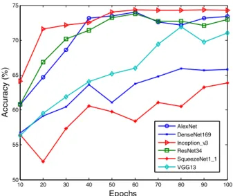
but with different epochs. In order to see the relationship between accuracy and epochs for different Deep Learning models, we plot them in a graph as shown in Fig. 4.
FIGURE 4. The relationship between Epochs and Accuracy.
In addition, we take epochs=60 as an example, showing the experimental results of the models with Top 3 accuracies in Table 6.
Generally speaking, the deep CNN approaches are better than traditional machine learning ones which need to extract the features from images before training. However, the results of our research show that different Deep Learning models with transfer learning have different abilities to detect plant disease severity.
Furthermore, the normalized confusion matrices of the Top 3 models are shown in Fig.5. From Fig. 4 and Table 6, we can see that the accuracies of different models are very close to each other. Comparatively, in all six Deep Learning models, Inception_v3 has the best accuracy of 74.38% in the experiments for the severity detection of plant disease when the training epochs are equal to 60. Then AlexNet is top 2 with accuracy 72.34%, followed by Resnet34 with accuracy 72.16%. Moreover, when the epochs are more than 60, the accuracy of Inception_v3 tends to be stable, but those of AlexNet and Resnet34 become unstable or even worse.
In addition, based on Fig.5, we find that Inception_v3 has a good balance in detecting three kinds of disease severities. Therefore, Inception_v3 with epochs=60 is chosen as the ‘best’ models, though its accuracy (74.38%) is not good enough.
TABLE 6.The experimental results of the models with top 3 accuracies.
FIGURE 5. The normalized confusion matrix of different models.
B. RESULTS AND DISCUSSION FOR DCGANs DATA AUGMENTATION
In order to improve the performance of the best model, Incep-tion_v3 with epochs=60, we employed DCGANs to augment the training dataset, and combined the original dataset with augmented data to retrain it.
The pictures comparing the original and DCGANs-generated images of three different classes are shown in Fig.6 (a) to (c). Moreover, for obtaining relatively high quality gener-ated images, we set the relgener-ated parameters of DCGAN to determine whether or not to save the generated images. For example, we set the error of Generator and Discriminator between the real value and network output less than 0.5, and the training epochs bigger than 50. Moreover, we manually select the quality generated images to get the planned aug-mentation size.
C. RESULTS AND DISCUSSION FOR MODEL PERFORMANCE IMPROVEMENT
After achieving enough augmented data, we mixed the origi-nal training images with the augmented ones to create a new training dataset, whereas the same test dataset was used to test the performance of the newly trained model.
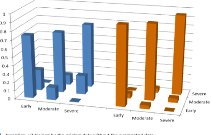
After using the new training dataset to retrain the Incep-tion_v3 with epochs=60, the experimental results show that the retrained model gets an improved performance with accuracy of 92.60% (about 20% higher than that of the model trained by the original training dataset, 74.38%). Furthermore, we obtained a good accuracy for each class. Fig.7 shows the confusion matrices of Inception_v3 trained
FIGURE 6. Original vs. generated images for different Classes.
FIGURE 7. The normalized confusion matrix of Inception_v3 trained without and with the augmented data.
by the original dataset and the one combined the original with augmented data.
V. CONCLUSION AND FUTURE WORK
A. CONCLUSION
In this work, we proposed the idea of classifying the HLB-infected citruses into different severity levels, which provides a good evidence for citrus farmers or growers to make corre-sponding decisions. Especially, finding HLB at the early time can not only protect the healthy citruses from being infected, but also can reduce the farmers’ financial loss.
According to the experimental results, Deep Learning model with deep transfer learning strategy are good choices for plant disease severity detection. Comparatively, Incep-tion_v3 with epochs=60 could be the first choice of selection for severity detection of plant disease. Furthermore, training epoch size is an important parameter influencing the perfor-mance of Deep Learning. It is depended on the size of dataset and the type of the model.
Besides, the technique of data augmentation based on DCGANs was employed to augment dataset size. By com-bining the original images with the augmented ones and using the same test dataset, the performance of the Deep Learning model was significantly improved.
Finally, it should be pointed out that this work could be an example on how to employ deep convolutional neural networks to detect plant diseases in general. In addition, early detection and prediction of plant or human diseases are the most promising research direction in the future, with different image datasets being created.
B. FUTURE WORK
It should be recognized that the datasets used in this work have some major limitations because the images in them are all from PlantVillage and crowdAI or generated by DCGANs, which have been preprocessed. In practical situ-ations, the results will be influenced by many factors such as illumination differences, sensor differences, cultivar, geo-graphic area, etc. Therefore, our work needs to be further assessed in more real-world scenarios. In our future work, we will create a dataset with images captured in the real environment and test what effects they will be for different Deep Learning models.
In addition, many traditional augmented methods such as flipping, translation, rotation, scaling, and shearing etc. can also be used to augment data. Consequently, comparing the DCGANs data augmentation with the traditional data aug-mentation could be one of our future works.
REFERENCES
[1] J. Amara, B. Bouaziz, and A. Algergawy, ‘‘A deep learning-based approach for banana leaf diseases classification,’’ inProc. LNI, Gesellschaft für Informatik, Bonn, Germany, 2017, pp. 79–88.
[2] M. Brahimi, M. Arsenovic, S. Laraba, S. Sladojevic, K. Boukhalfa, and A. Moussaoui, ‘‘Deep learning for plant diseases: Detection and saliency map visualisation,’’ inHuman and Machine Learning: Visible, Explain-able, Trustworthy Transparent, J. Zhou and F. Chen, Eds. Cham, Switzerland: Springer, 2018, pp. 93–117.
[3] K. P. Ferentinos, ‘‘Deep learning models for plant disease detection and diagnosis,’’Comput. Electron. Agricult., vol. 145, pp. 311–318, Feb. 2018, doi:10.1016/j.compag.2018.01.009.
[4] Y. Lu, S. Yi, N. Zeng, Y. Liu, and Y. Zhang, ‘‘Identification of rice diseases using deep convolutional neural networks,’’Neurocomputing, vol. 267, pp. 378–384, Dec. 2017, doi:10.1016/j.neucom.2017.06.023.
[5] S. P. Mohanty, D. P. Hughes, and M. Salathé, ‘‘Using deep learning for image-based plant disease detection,’’Frontiers Plant Sci., vol. 7, p. 1419, Sep. 2016, doi:10.3389/fpls.2016.01419.
[6] A. Ramcharan, K. Baranowski, P. McCloskey, B. Ahmed, J. Legg, and D. P. Hughes, ‘‘Deep learning for image-based cassava disease detection,’’ Frontiers Plant Sci., vol. 8, p. 1852, Oct. 2017, doi: 10.3389/fpls.2017.01852.
[7] S. Sladojevic, M. Arsenovic, A. Anderla, D. Culibrk, and D. Stefanovic, ‘‘Deep neural networks based recognition of plant diseases by leaf image classification,’’Comput. Intell. Neurosci., vol. 2016, pp. 1–11, May 2016, doi:10.1155/2016/3289801.
[8] S. B. Patil and S. K. Bodhe, ‘‘Leaf disease severity measurement using image processing,’’Int. J. Eng. Tech., vol. 3, no. 5, pp. 297–301, 2011. [9] C. H. Bock, G. H. Poole, P. E. Parker, and T. R. Gottwald, ‘‘Plant disease
severity estimated visually, by digital photography and image analysis, and by hyperspectral imaging,’’Crit. Rev. Plant Sci., vol. 29, no. 2, pp. 59–107, Mar. 2010, doi:10.1080/07352681003617285.
[10] I. Dhau, E. Adam, O. Mutanga, and K. K. Ayisi, ‘‘Detecting the severity of maize streak virus infestations in maize crop usingin situhyperspectral data,’’Trans. Roy. Soc. South Afr., vol. 73, no. 1, pp. 8–15, Jan. 2018, doi: 10.1080/0035919X.2017.1370034.
[11] G. Wang, Y. Sun, and J. Wang, ‘‘Automatic image-based plant dis-ease severity estimation using deep learning,’’Comput. Intell. Neurosci., vol. 2017, pp. 1–8, Jul. 2017, doi:10.1155/2017/2917536.
[12] Agricultural Research Service, USDA. (Mar. 13, 2020). Huanglong-bing (Citrus Greening): What ARS Is Doing. [Online]. Available: https://www.ars.usda.gov/oc/br/citrusgreening/index/.
[13] Agricultural Research Council. (2017). Citrus Huanglongbing (HLB). [Online]. Available: http://www.arc.agric.za/arc-ppri/Fact
[14] AQIS. Citrus Huanglongbing (Greening). Accessed: Jul. 25, 2019. [Online]. Available: https://www.cabi.org/isc/datasheet/16567
[15] A. Radford, L. Metz, and S. Chintala, ‘‘Unsupervised representation learning with deep convolutional generative adversarial networks,’’ 2015, arXiv:1511.06434. [Online]. Available: http://arxiv.org/abs/1511.06434 [16] J. G. A. Barbedo, ‘‘Factors influencing the use of deep learning for
plant disease recognition,’’Biosyst. Eng., vol. 172, pp. 84–91, Aug. 2018. 10.1016/j.biosystemseng.2018.05.013.
[17] D. P. Hughes and M. Salathe, ‘‘An open access repository of images on plant health to enable the development of mobile disease diagnostics,’’ 2015, arXiv:1511.08060. [Online]. Available: https://arxiv.org/abs/1511.08060
[18] CrowdAI. (2019). PlantVillage Disease Classification Challenge. [Online]. Available: https://www.crowdai.org/challenges/1/dataset_files [19] A. Krizhevsky, ‘‘One weird trick for parallelizing convolutional
neural networks,’’ 2014, arXiv:1404.5997. [Online]. Available: http://arxiv.org/abs/1404.5997
[20] M. Zahangir Alom, T. M. Taha, C. Yakopcic, S. Westberg, P. Sidike, M. Shamima Nasrin, B. C Van Esesn, A. A S. Awwal, and V. K. Asari, ‘‘The history began from AlexNet: A comprehensive survey on deep learning approaches,’’ 2018,arXiv:1803.01164. [Online]. Available: http://arxiv.org/abs/1803.01164
[21] K. Simonyan and A. Zisserman, ‘‘Very deep convolutional networks for large-scale image recognition,’’ 2014,arXiv:1409.1556. [Online]. Avail-able: http://arxiv.org/abs/1409.1556
[22] K. He, X. Zhang, S. Ren, and J. Sun, ‘‘Deep residual learning for image recognition,’’ inProc. IEEE Conf. Comput. Vis. Pattern Recognit. (CVPR), Jun. 2016, pp. 770–778.
[23] A. Khan, A. Sohail, U. Zahoora, and A. Saeed Qureshi, ‘‘A sur-vey of the recent architectures of deep convolutional neural net-works,’’ 2019,arXiv:1901.06032. [Online]. Available: http://arxiv.org/ abs/1901.06032
[24] C. Szegedy, V. Vanhoucke, S. Ioffe, J. Shlens, and Z. Wojna, ‘‘Rethinking the inception architecture for computer vision,’’ inProc. IEEE Conf. Comput. Vis. Pattern Recognit. (CVPR), Jun. 2016, pp. 2818–2826. [25] F. N. Iandola, S. Han, M. W. Moskewicz, K. Ashraf, W. J. Dally, and
K. Keutzer, ‘‘SqueezeNet: AlexNet-level accuracy with 50x fewer param-eters and <0.5MB model size,’’ 2016,arXiv:1602.07360. [Online]. Avail-able: http://arxiv.org/abs/1602.07360
[26] G. Huang, Z. Liu, L. van der Maaten, and K. Q. Weinberger, ‘‘Densely connected convolutional networks,’’ 2016,arXiv:1608.06993. [Online]. Available: http://arxiv.org/abs/1608.06993
[27] S. Sharma. (2019).Epoch vs Batch Size vs Iterations. [Online]. Available: https://towardsdatascience.com/epoch-vs-iterations-vs-batch-size-4dfb9c7ce9c9
[28] Y. Bengio, ‘‘Practical recommendations for gradient-based training of deep architectures,’’ 2012, arXiv:1206.5533. [Online]. Available: http://arxiv.org/abs/1206.5533
[29] D. Masters and C. Luschi, ‘‘Revisiting small batch training for deep neural networks,’’ 2018, arXiv:1804.07612. [Online]. Available: http://arxiv.org/abs/1804.07612
[30] M. Frid-Adar, E. Klang, M. Amitai, J. Goldberger, and H. Greenspan, ‘‘Synthetic data augmentation using GAN for improved liver lesion classification,’’ 2018, arXiv:1801.02385. [Online]. Available: http://arxiv.org/abs/1801.02385
[31] I. J. Goodfellow, J. Pouget-Abadie, M. Mirza, B. Xu, D. Warde-Farley, S. Ozair, A. Courville, and Y. Bengio, ‘‘Generative adversarial networks,’’ 2014, arXiv:1406.2661. [Online]. Available: http://arxiv.org/abs/1406.2661
[32] N. Inkawhich. (2017). DCGAN Tutorial. [Online]. Available: https://pytorch.org/tutorials/beginner/dcgan_faces_tutorial.html [33] A. Odena, C. Olah, and J. Shlens, ‘‘Conditional image synthesis with
auxiliary classifier GANs,’’ 2016,arXiv:1610.09585. [Online]. Available: http://arxiv.org/abs/1610.09585
[34] D. Berthelot, T. Schumm, and L. Metz, ‘‘BEGAN: Boundary equilib-rium generative adversarial networks,’’ 2017,arXiv:1703.10717. [Online]. Available: http://arxiv.org/abs/1703.10717
[35] J.-Y. Zhu, R. Zhang, D. Pathak, T. Darrell, A. A. Efros, O. Wang, and E. Shechtman, ‘‘Toward multimodal Image-to-Image translation,’’ 2017, arXiv:1711.11586. [Online]. Available: http://arxiv.org/abs/1711.11586 [36] E. Linder-Norén. (2019). PyTorch Implementations of Generative
Adversarial Networks. [Online]. Available: https://github.com/erikli ndernoren/PyTorch-GAN
[37] Torch Contributors. (2018).Pytorch Documentation. [Online]. Available: https://pytorch.org/docs/stable/index.html
[38] M. Arsenovic. (2018).DeepLearning_PlantDiseases. [Online]. Available: https://github.com/MarkoArsenovic/DeepLearning_PlantDiseases [39] PyTorch. (2019). CrossEntropyLoss. [Online]. Available:
https://pytorch.org/docs/stable/nn.html#torch.nn.CrossEntropyLoss
QINGMAO ZENG received the M.S. degree in applied mathematics from the Xi’an University of Science and Technology, Xi’an, China, in 2005, and the Ph.D. degree in biomathematics from South China Agricultural University, Guangzhou, China, in 2015.
He is currently a full-time Lecturer with the Department of Mathematics, College of Mathe-matics and InforMathe-matics, South China Agricultural University. From 2018 to 2019, he was a Visiting Scholar with the University of Hull (Xinhui Ma, the second author of this article, was his supervisor). His research interests include artificial neural networks, fuzzy mathematics, plant species identification, and plant disease detection.
Dr. Zeng was a recipient of the Excellent Individual of South China Agricultural University, in 2011, 2013, and 2015, and the Guangdong Provin-cial Excellent Instructor of China Undergraduate Mathematical Contest in Modeling, in 2016.
XINHUI MA received the Ph.D. degree in mechanical engineering from the University of Birmingham, U.K., in 2007.
He was a Research Fellow with the University of Strathclyde and a Research Associate with the University of Cambridge. He is currently a Lec-turer with the Department of Computer Science and Technology, University of Hull, U.K. He is the author of more than 20 articles. His research inter-ests include health informatics, biomedical image analysis, machine learning, data visualization, computer vision, computer graphics, virtual reality, and augmented reality. His research has been funded by EPSRC.
BAOPING CHENGreceived the M.S. and Ph.D. degrees in plant pathology from Nanjing Agricul-tural University, Nanjing, China, in 2008 and 2011, respectively.
He is currently an Associate Professor with the Plant Protection Institute, Guangdong Academy of Agriculture. His research interests include detec-tion and control of citrus disease and pathogenic mechanism research of citrus disease. He was a recipient of the Excellent Individual of Guangdong Academy of Agriculture, in 2014 and 2015.
ERXUN ZHOUreceived the B.S. degree in plant protection from Hainan University, Haikou, China, in 1986, and the Ph.D. degree in plant pathology from Nanjing Agricultural University, Nanjing, China, in 1994.
From 1986 to 1989, he was a full-time Teaching Assistant with the Department of Plant Protection, Hainan University. From 1994 to 1995, he was a Lecturer with the Department of Plant Protection, South China Agricultural University, Guangzhou, China. From 1995 to 1997, he was a Postdoctoral Research Fellow with the Department of Plant Pathology, South China Agricultural University, where he was an Associate Professor, from 1997 to 2004. From December 2003 to June 2004, he was a Visiting Scientist with the Citrus Research and Education Center, University of Florida, FL, USA. From July 2004 to August 2005, he was a Visiting Scientist with the USDA-ARS Dale Bumpers National Rice Research Center/Rice Research and Extension Center, University of Arkansas, Stuttgart, AR, USA. From June 2009 to May 2010, he was a Visiting Scientist with the Children’s Hospital, Louisiana State University Health Science Center, New Orleans, LA, USA. Since 2004, he has been a Professor with the Department of Plant Pathology, South China Agricultural University. His research interests include the plant diseases and their control, fungal biology, genetics and genomics, host–pathogen interactions, plant disease resistance, and functional genomics of pant pathogens.
Prof. Zhou was a member of Chinese Society for Plant Pathology, Myco-logical Society of China, and The American PhytopathoMyco-logical Society, and the Editorial Board Member ofChinese Journal of Tropical Cropsand Journal of Tropical Biology.
WEI PANGreceived the Ph.D. degree in comput-ing science from the University of Aberdeen, U.K., in 2009.
He is currently an Associate Professor with Heriot-Watt University, Edinburgh, U.K. He is also an Honorary Senior Lecturer with the University of Aberdeen and a member of the Edinburgh Centre for Robotics. He has authored more than 100 arti-cles, including more than 50 journal articles. His research interests include bio-inspired computing, data mining, machine learning, and qualitative reasoning. His research has been funded by EPSRC, ESRC, BBSRC, Royal Society, Royal Society of Edinburgh, and most recently, Cancer Research U.K.
Dr. Pang was a recipient of the Best Paper Award at the 19th Annual U.K. Workshop on Computational Intelligence (UKCI 2019) and the Best Paper Runner Up Award at the 12th International Conference on Advanced Data Mining and Applications (ADMA 2016).