University of Wollongong
University of Wollongong
Research Online
Research Online
Centre for Statistical & Survey Methodology
Working Paper Series
Faculty of Engineering and Information
Sciences
2009
Borrowing strength over space in small area estimation: Comparing
Borrowing strength over space in small area estimation: Comparing
parametric, semi-parametric and non-parametric random effects and
parametric, semi-parametric and non-parametric random effects and
M-quantile small area models
quantile small area models
R. Chambers
University of Wollongong, [email protected]
N. Tzavidis
University of Manchester
N. Salvati
University of Pisa
Follow this and additional works at: https://ro.uow.edu.au/cssmwp
Recommended Citation
Recommended Citation
Chambers, R.; Tzavidis, N.; and Salvati, N., Borrowing strength over space in small area estimation: Comparing parametric, semi-parametric and non-parametric random effects and M-quantile small area models, Centre for Statistical and Survey Methodology, University of Wollongong, Working Paper 12-09, 2009, 13p.
https://ro.uow.edu.au/cssmwp/32
Research Online is the open access institutional repository for the University of Wollongong. For further information contact the UOW Library: [email protected]
Copyright © 2008 by the Centre for Statistical & Survey Methodology, UOW. Work in progress,
no part of this paper may be reproduced without permission from the Centre.
Centre for Statistical & Survey Methodology, University of Wollongong, Wollongong NSW
Centre for Statistical and Survey Methodology
The University of Wollongong
Working Paper
12-09
Borrowing strength over space in small area estimation: Comparing
parametric, semi-parametric and non-parametric random effects and
M-quantile small area models
Borrowing strength over space in small area estimation: Comparing parametric, semi-parametric
and non-parametric random effects and M-quantile small area models
Ray Chambers1, Nikos Tzavidis2, Nicola Salvati3
Centre for Statistical and Survey Methodology School of Mathematics and Applied Statistics, University of Wollongong1 Centre for Census and Survey Research, University of Manchester2
Dipartimento di Statistica e Matematica Applicata all’Economia, Universit`a di Pisa, Italy3 Abstract
In recent years there have been significant developments in model-based small area methods that incorporate spatial infor-mation in an attempt to improve the efficiency of small area estimates by borrowing strength over space. A popular approach parametrically models spatial correlation in area effects using Simultaneous Autoregressive (SAR) random effects models. An alternative approach incorporates the spatial information via M-quantile Geographically Weighted Regression (GWR), which fits a local model to the M-quantiles of the conditional distribution of the outcome variable given the covariates. A further approach uses spline approximations to fit nonparametric unit level nested error regression and M-quantile regression models that reflect spatial variation in the data and then uses these nonparametric models for small area estimation. In this presentation we contrast the performance of these alternative small area models using data with geographical information. We also examine how these models perform when estimation is for out of sample areas i.e. areas with zero sample, and discuss issues related to estimation of mean squared error of the resulting small area estimators. Our analysis is illustrated using simulations based on data from the U.S. Environmental Protection Agency’s Environmental Monitoring and Assessment Program.
Keywords: Spatial information; Robust regression; Iteratively Reweighted Least Squares; Nonparametric smoothing.
1 Introduction
In recent years there have been significant developments in model-based small area estimation. The most popular approach to small area estimation employs random effects models for estimating domain specific parameters (Rao, 2003). An alternative approach to small area estimation that relaxes the parametric assumptions of random effects models by employing M-quantile models was recently proposed by Chambers & Tzavidis (2006). Typically, random effects models assume independence of the random area effects. This independence assumption is also implicit in M-quantile small area models. In economic, environ-mental and epidemiological applications, however, observations that are spatially close may be more related than observations that are further apart. This spatial correlation can be accounted for by extending the random effects model to allow for spatially correlated area effects using, for example, a Simultaneous Autoregressive (SAR) model (Anselin, 1988; Cressie, 1993). The application of Simultaneous Autoregressive models to small area estimation enables researchers to borrow strength over space and hence improve the precision of small area estimates. In this context, Singh et al. (2005) and Pratesi & Salvati (2008) proposed the use of the Spatial Empirical Best Linear Unbiased Predictor (SEBLUP).
SAR models allow for spatial correlation in the error structure. An alternative approach to incorporating the spatial infor-mation in the regression model is by assuming that the regression coefficients vary spatially across the geography of interest. Geographically Weighted Regression (GWR) (Brundson et al., 1996; Fotheringham et al., 1997, 2002; Yu & Wu, 2004) extends the traditional regression model by allowing local rather than global parameters to be estimated. That is, GWR directly models spatially non-stationarity in the mean structure of the model. In a recent paper Salvati et al. (2008) proposed an M-quantile GWR small area model. In doing so, the authors first proposed an extension to the GWR model, M-quantile GWR model, i.e. a locally robust model for the M-quantiles of the conditional distribution of the outcome variable given the covariates. This model was then used to define a predictor of the small area characteristic of interest that accounts for spatial structure of the data. The M-quantile GWR small area model integrates the concepts of robust small area estimation and borrowing strength over space within a unified modeling framework.
When the functional form of the relationship between the response variable and the covariates is unknown or has a com-plicated functional form, an approach based on use of a nonparametric regression model using penalized splines can offer significant advantages compared with one based on a linear model. By expressing the spline coefficients in the model as ran-dom effects, Ruppert et al. (2003) show how fitting a p-spline model is equivalent to fitting a linear mixed model. On the basis of this property, Opsomer et al. (2008) have recently proposed a new approach to SAE that extends the unit level nested error regression model (Battese et al., 1988) by combining small area random effects with a p-spline regression model. Pratesi et al. (2008) have extended this approach to the M-quantile method for the estimation of the small area parameters using a nonparametric specification of the conditional M-quantile of the response variable given the covariates. The use of bivariate p-spline approximations to fit nonparametric unit level nested error and M-quantile regression models allows for reflecting spatial variation in the data and then uses these nonparametric models for small area estimation.
In this paper we contrast SAR, unit level nested error p-spline regression, M-quantile GWR and M-quantile spline models in terms of their performance using data with geographical information. We also examine whether estimation for out of sample areas i.e. areas with zero sample sizes can be improved using models that borrow strength over space. The structure of the paper is as follows. In section 2 we review unit level mixed models with independent and spatially correlated random area effects for small area estimation. In section 3 we present M-quantile and M-quantile GWR models for small area estimation. In section 4 we describe the nonparametric unit level nested error and M-quantile regression models. Estimation of the mean squared error of the resulting small area predictors under modeling approaches is discussed. For exploring the research questions of this paper we employ a real survey datasets: data from the U.S. Environmental Protection Agency’s Environmental Monitoring and Assessment Program (EMAP). The dataset contains geo-referenced and in section 5 we use design-based simulation experiments for assessing the performance of the different small area predictors and their associated estimates of mean squared error considered in this paper. Finally, in section 6 we summarize our main findings.
2 Unit level mixed models for small area estimation
Letxij denote a vector ofpauxiliary variables for each population unitjin small areaiand assume that information for the
variable of interestyis available only from the sample. The target is to use the data to estimate various area-specific quantities. A popular approach for this purpose is to use mixed effects models with random area effects. A linear mixed effects model is
yij =xTijβ+zijγi+ij, j= 1. . . , nii= 1, . . . , d (1)
whereβis thep×1vector of regression coefficients,γi denotes a random area effect that characterizes differences in the
conditional distribution ofy givenxbetween thedsmall areas, zij is a constant whose value is known for all units in the
population andij is the error term associated with thej-th unit within thei-th area. Conventionally,γi andijare assumed
to be independent and normally distributed with mean zero and variancesσγ2andσ2respectively. The Empirical Best Linear
Unbiased Predictor (EBLUP) of the mean for small areai(Battese et al., 1988; Rao, 2003) is then
ˆ mM Xi =N− 1 i h X j∈si yj+ X j∈ri ˆ yj i (2)
whereyˆj =xTjβˆ +zjγˆi,sidenotes thenisampled units in areai,ridenotes the remainingNi−niunits in the areaiandβˆ
andγˆiare obtained by substituting an optimal estimate of the covariance matrix of the random effects in (1) into the best linear
unbiased estimator ofβand the best linear unbiased predictor ofγirespectively.
Model (1) can be extended to allow for correlated random area effects. Let the deviationsvfrom the fixed part of the model XTβbe the result of an autoregressive process with parameterρand proximity matrixW(Anselin, 1988; Cressie, 1993), then
v=ρWv+γ→v= (I−ρW)−1γ (3)
whereIis ad×didentity matrix. Combining (1) and (3), withεindependent ofv, the model with spatially correlated errors can be expressed as
y=XTβ+Z(I−ρW)−1γ+ε. (4)
The error termvthen has ad×dSimultaneously Autoregressive (SAR) dispersion matrix given by G=σ2γh(I−ρWT)(I−ρW)i
−1
. (5)
TheWmatrix describes the neighbourhood structure of the small areas andρdefines the strength of the spatial relationship between the random effects of neighbouring areas.
Under (4), the Spatial Best Linear Unbiased Predictor (Spatial BLUP) of the small area mean and its empirical version (SEBLUP) are obtained following Henderson (1975). In particular, theSEBLUPof the small area mean,mi, is
ˆ mM X/SARi =Ni−1h X j∈si yj+ X j∈ri ˆ yj i (6)
2.1 MSE estimation for small area estimates under the SAR mixed model
An expression for the mean squared error (MSE) under theSEBLUP model and its estimator are obtained following the results of Kackar & Harville (1984), Prasad & Rao (1990) and Datta & Lahiri (2000). More specifically, the MSE estimator consists of three components denoted byg1,g2andg3:
M SE[ ˆmM X/SARi ] =g1i(σγ2, σ 2 ε, ρ) +g2i(σ2γ, σ 2 ε, ρ) +g3i(σ2γ, σ 2 ε, ρ).
The components of the MSE are due to the variability associated with the estimation of the random effects (g1), the estimation ofβ(g2) and the estimation of(σ2γ, σε2, ρ)(g3). Note that due to the introduction of the additional parameterρ, componentg3of the MSE is not the same as in the case of theEBLUP(Prasad & Rao, 1990).
In practical applications the predictormˆM X/SARi has to be associated with an estimator ofM SE[ ˆmM X/SARi ]. Following the results of Harville & Jeske (1992) and Zimmerman & Cressie (1992) an approximately unbiased mean squared error estimator of is given by
mse[ ˆmM X/SARi ]≈g1i(ˆσ2γ,σˆε2,ρ) +ˆ g2i(ˆσγ2,σˆε2,ρ) + 2gˆ 3i,(ˆσ2γ,σˆε2,ρ)ˆ (7)
whenσˆ2
γ,σˆ2ε,ρˆare REML estimators. See Singh et al. (2005) and Pratesi & Salvati (2008) for details.
3 M-quantile models for small area estimation
A recently proposed approach to small area estimation is based on the use of M-quantile models (Chambers & Tzavidis, 2006; Tzavidis et al., 2008). A linear M-quantile regression model is one where the qthM-quantile Q
q(x;ψ)of the conditional
distribution ofygivenxsatisfies
Qq(X;ψ) =XTβψ(q). (8)
Hereψdenotes the influence function associated with the M-quantile. For specifiedqand continuousψ, an estimateβˆψ(q)of
βψ(q)is obtained via iterative weighted least squares.
Following Chambers & Tzavidis (2006) an alternative to random effects for characterizing the variability across the popu-lation is to use the M-quantile coefficients of the popupopu-lation units. For unitjwith valuesyjandxj, this coefficient is the value
θj such thatQθj(xj;ψ) =yj. These authors observed that if a hierarchical structure does explain part of the variability in the population data, units within clusters (areas) defined by this hierarchy are expected to have similar M-quantile coefficients. When the conditional M-quantiles are assumed to follow a linear model, withβψ(q)a sufficiently smooth function ofq, this suggests a predictor ofmiof the form
ˆ mM Qi =Ni−1h X j∈si yj+ X j∈ri {xTjβˆψ(ˆθi)} i (9)
whereθˆiis an estimate of the average value of the M-quantile coefficients of the units in areai. Typically this is the average of
estimates of these coefficients for sample units in the area. These unit level coefficients are estimated by solvingQˆqj(xj;ψ) =
yjforqjwithQˆq denoting the estimated value of (8) atq. When there is no sample in areaithenθˆi= 0.5.
Tzavidis et al. (2008) refer to (9) as the ‘naive’ M-quantile predictor and note that this can be biased. To rectify this problem these authors propose a bias adjusted M-quantile predictor ofmi that is derived as the mean functional of the Chambers &
Dunstan (1986) (CD hereafter) estimator of the distribution function and is given by
ˆ mM Q/CDi = Z +∞ −∞ tdFˆi(t) =Ni−1 h X j∈si yj+ X j∈ri {xTjβˆψ(ˆθi)}+ Ni−ni ni X j∈si {yj−xTjβˆψ(ˆθi)} i . (10)
3.1 M-quantile geographically weighted model for small area estimation
SAR mixed models are global models i.e. with such models we assume that the relationship we are modeling holds everywhere in the study area and we allow for spatial correlation at different hierarchical levels in the error structure. One way of incor-porating the spatial structure of the data in the M-quantile small area model is via an M-quantile GWR model (Salvati et al., 2008). Unlike SAR mixed models, M-quantile GWR are local models that allow for a spatially non-stationary process in the mean structure of the model.
Givennobservations at a set ofLlocations{ul;l = 1, . . . , L;L 6 n}withnldata values{(yjl,xjl);j = 1, . . . , nl}
observed at locationul, an M-quantile GWR model is defined as
Qq(X;ψ, u) =XTβψ(u;q) (11)
where nowβψ(u;q)varies withuas well as withq. The M-quantile GWR is a local model for the entire conditional distribution
-not just the mean- ofygivenx. Estimates ofβψ(u;q)in (11) can be obtained by solving
L X l=1 w(ul, u) nl X j=1 ψq{yjl−xTjlβψ(u;q)}xjl=0 (12)
whereψq(t) = 2ψ(s−1t){qI(t >0) + (1−q)I(t60)}andsis a suitable robust estimate of scale such as the median absolute
deviation (MAD) estimates =median|yjl−xTjlβψ(u;q)|/0.6745. It is also customary to assume a Huber type influence
function although other influence functions are also possible
ψ(t) =tI(−c6t6c) +sgn(t)I(|t|> c).
Providedcis bounded away from zero, an iteratively re-weighted least squares algorithm can then be used to solve (12), leading to estimates of the form
ˆ βψ(u;q) = n XTW∗(u;q)Xo −1 XTW∗(u;q)y. (13)
In (13)y is the vector ofnsampley values andXis the corresponding design matrix of ordern×pof samplexvalues. The matrixW∗(u;q)is a diagonal matrix of ordernwith entries corresponding to a particular sample observation and equal to the product of this observation’s spatial weight, which depends on its distance from locationu, with the weight that this observation has when the sample data are used to calculate the ‘spatially stationary’ M-quantile estimateβˆψ(q). At this point we should mention that the spatial weight is derived from a spatial weighting function whose value depends on the distance from sample locationultousuch that sample observations with locations close toureceive more weight than those further
away. One popular approach to defining such a weighting function is to use
w(ul, u) =exp
n
−0.5(d(ul,u)/b) 2o,
whered(ul,u)denotes the Euclidean distance betweenulanduandbis the bandwidth, which can be optimally defined using a least squares criterion (Fotheringham et al., 2002). It should be noted, however, that alternative weighting functions, for example the bi-square function, can also be used.
Salvati et al. (2008) also proposed a reduced M-quantile GWR that combines local intercepts with global slopes and is defined as
Qq(X;ψ, u) =XTβψ(q) +δψ(u;q). (14)
This is fitted in two steps. At the first step we ignore the spatial structure in the data and estimateβψ(q) directly via the
iterative re-weighted least squares algorithm used to fit the standard linear M-quantile regression model (8). At the second step geographic weighting is applied to estimateδψ(u;q)using
ˆ δψ(u;q) =n−1 L X l=1 w(ul, u) nl X j=1 ψq{yjl−xTjlβˆψ(q)}.
Hereafter we refer to (11) and (14) as theMQGWRandMQGWR-LI(Local Intercepts) models respectively.
The primary aim of this paper is to employ theMQGWRandMQGWR-LImodels for estimating the area i meanmiofy.
Following Chambers & Tzavidis (2006) this can be done by first estimating the M-quantile GWR coefficients{qj;j ∈s}of
the sampled population units without reference to the small areas of interest. A grid-based interpolation procedure for doing this under (8) is described in Chambers & Tzavidis (2006) and can be directly used with the M-quantile GWR models (11) and (14). In particular, we adapt this approach with M-quantile GWR models by first defining a fine grid of q values over the interval(0,1)and then use the sample data to fit (11) or (14) for each distinct value ofqon this grid and at each sample location. The M-quantile GWR coefficient for unitj with valuesyj andxj at locationuj is computed by interpolating over
this grid to find the valueqjsuch thatQqj(xj;ψ, uj) =yj.
Provided there are sample observations in areai, an area-specific M-quantile GWR coefficient,θˆi, can be defined as the
average value of the sample M-quantile GWR coefficients in area i. Following Salvati et al. (2008), the bias-adjusted M-quantile GWR predictor of the mean in small areaiis
ˆ mM QGW R/CDi =Ni−1h X j∈si yj+ X j∈ri ˆ Qθˆi(xj;ψ, uj) + Ni−ni ni X j∈si {yj−Qˆθˆi(xj;ψ, uj)} i . (15)
whereQˆθˆi(xj;ψ, uj)is defined either via theMQGWRmodel (11) or via theMQGWR-LI(14).
3.2 MSE estimation for small area estimates under the M-quantile GWR model
Mean squared error estimation for the M-quantile GWR small area estimates is based on the Chambers et al. (2008) estimator and is also described in Salvati et al. (2008). To start with we note that (15) can be expressed as a weighted sum of the sample
y-values
ˆ
where wi= Ni ni 1i+ X j∈ri HTijxj− Ni−ni ni X j∈si HTijxj. (17)
Here 1i is then-vector with jthcomponent equal to one whenever the corresponding sample unit is in area iand is zero
otherwise and Hij = n XTW∗(uj; ˆθi)X o−1 XTW∗(uj; ˆθi).
Given the linear representation (16), an estimator of a first order approximation to the mean squared error of this predictor can be computed following standard methods of robust mean squared error estimation for linear predictors of population quantities (Royall & Cumberland, 1978). Putwi= (wij)this estimator is of the form
v( ˆmM QGW R/CDi ) =Ni−2 X k:nk>0 X j∈sk λijk n yj−Qˆθˆ k(xj;ψ, uj) o2 (18) whereλijk= n (wij−1)2+ (ni−1)−1(Ni−ni) o I(k=i) +w2 jkI(k6=i).
4 Nonparametric small area models
Although very useful in many situations, linear mixed models depend on distributional assumptions for the random part of the model and do not easily allow for outlier robust inference. In addition, the fixed part of the model may not be flexible enough to handle cases in which the relationship between the variable of interest and the covariates is more complex than that assumed by a linear model. Opsomer et al. (2008) extend model (1) to the case in which the small area random effects can be combined with a smooth, non-parametrically specified trend. In particular, in the simplest case
yij =m(x1ij) +zijγi+ij, j= 1. . . , nii= 1, . . . , d, (19)
wherem(·)is an unknown smooth function of the variablex1. The estimator of the small area mean is
ˆ mN P M Xi =Ni−1h X j∈si yj+ X j∈ri ˆ yj i (20)
as in (2) whereyˆj = ˆm(x1ij) +zijˆγi. By using penalized splines as the representation for the non-parametric trend, Opsomer
et al. (2008) express the non-parametric small area estimation model as a random effects model withm(xˆ 1ij) = ˆβ0+ ˆβ1x1ij+
aijδ. Then theyˆj value includes the spline function, which is treated as a random effect, and the small area random effect.
The latter can be easily extended to handle bivariate smoothing and additive modeling. These authors proposed and studied the theoretical properties of the mean squared error of (20). They extended the results of Prasad & Rao (1990) and Das et al. (2008) to the case of a spline-based random effect. Opsomer et al. (2008) also proposed a bootstrap estimator for the MSE, which performs reasonably well, but is computationally intensive.
Pratesi et al. (2008) have extended this approach to the M-quantile method for the estimation of the small area parameters using a nonparametric specification for the conditional M-quantiles of the response variable given the covariates. When the functional form of the relationship between theq-th M-quantile and the covariates deviates from the assumed one, the linear M-quantile regression model can lead to biased estimators of the small area parameters. When the relationship between theq-th M-quantile and the covariates is not linear, a p-splines M-quantile regression model may have significant advantages compared to the linear M-quantile model.
The small area estimator of the mean may be taken as in (9) where the unobserved value for population uniti ∈ rj is
predicted using
ˆ
yij =xijβˆψ(ˆθi) +aijνˆψ(ˆθi),
whereβˆψ(ˆθi)andνˆψ(ˆθi)are the coefficient vectors of the parametric and spline components, respectively, of the fitted
p-splines M-quantile regression function atθˆi. In case of p-splines M-quantile regression models the bias-adjusted estimator for
the mean is given by
ˆ mN P M Q/CDi = 1 Ni n X j∈Ui ˆ yij+ Ni ni X i∈si (yij−yˆij) o , (21)
whereyˆijdenotes the predicted values for the population units insiand inUi.
Following the approach described in Chambers et al. (2008), for fixedq, themˆN P M Q/CDi in (21) can be written as linear combination of the observedyij. The derived weights are treated as fixed and a ’plug in’ estimator of the mean squared error
estimators (Royall & Cumberland, 1978) and by following the results due to Chambers et al. (2008). See Salvati et al. (2008a) for details.
The use of bivariate p-spline approximations to fit nonparametric unit level nested error and M-quantile regression models allows for reflecting the spatial variation in the data and then uses these nonparametric models for small area estimation.
In particular, for M-quantile models, as we have just dealt with flexible smoothing of quantiles in scatterplots, we can now handle the way in which two continuous variables affect the quantiles of the response without any structural assumptions:
Qq(x1, x2, ψ) = ˜mψ,q(x1, x2), i.e. we can deal withbivariatesmoothing. It is of central interest in a number of application areas as environment and public health. It has particular relevance when geographically referenced responses need to be converted to maps. As seen earlier, p-splines rely on a set of basis functions to handle nonlinear structures in the data. Bivariate smoothing requires bivariate basis functions; Ruppert et al. (2003) advocate the use of radial basis functions to deriveLow-rank thin plate splines. In particular, the following model is assumed at quantileqfor uniti:
mψ,q[x1i, x2i;βψ(q),γψ(q)] =β0ψ(q) +β1ψ(q)x1i+β2ψ(q)x2i+aiνψ(q). (22)
Hereziis thei-th row of the followingn×Kmatrix
A= [C(˜xi−κk)]16i6n
16k6K
[C(κk−κk0)]−11/2
6k,k06K, (23)
whereC(t) =||t||2log||t||,x˜
i= (x1i, x2i)andκk,k= 1, . . . , Kare knots. See Pratesi et al. (2008) for details on this.
The choice of knots in two dimensions is more challenging than in one. One approach could be that of laying down a rectangular lattice of knots, but this has a tendency to waste a lot of knots when the domain defined byx1 andx2 has an irregular shape. In one dimension a solution to this issue is that of using quantiles. However, the extension of the notion of quantiles to more than one dimension is not straightforward. Two solutions suggested in literature that provide a subset of observations nicely scattered to cover the domain arespace filling designs(Nychka & Saltzman, 1998) and the clara algorithm (Kaufman & Rousseeuw, 1990). The first one is based on the maximal separation principle ofKpoints among the unique
˜
xi and is implemented in the fields package of theRlanguage. The second one is based on clustering and selects K
representative objects out ofn; it is implemented in the packageclusterofR.
4.1 A note on small area estimation for out of sample areas
In some situations we are interested in estimating small area characteristics for domains (areas) with no sample observations. The conventional approach to estimating a small area characteristic, say the mean, in this case is synthetic estimation.
Under the mixed model (1) or the SAR mixed model (4) the synthetic mean predictor for out of sample areaiis
ˆ
mM X/SY N T Hi =Ni−1 X
j∈Ui
xTjβˆ, (24)
whereUi=siSri.
Under M-quantile model (8) the synthetic mean predictor for out of sample areaiis
ˆ
mM Q/SY N T Hi =Ni−1 X
j∈Ui
xTjβˆψ(0.5). (25)
We note that with synthetic estimation all variation in the area-specific predictions comes from the area-specific auxiliary information. One way of potentially improving the conventional synthetic estimation for out of sample areas is by using a model that borrows strength over space such as an M-quantile GWR model and nonparametric unit level nested error and M-quantile regression models. In this case a synthetic-type mean predictors for out of sample areaiare defined by
ˆ mM QGW R/SY N T Hi =Ni−1X j∈Ui ˆ Q0.5(xj;ψ, uj) (26) ˆ mN P M X/SY N T Hi =Ni−1 X j∈Ui ˆ m(x1ij, uj) (27) ˆ mN P M Q/SY N T Hi =Ni−1 X j∈Ui [xijβˆψ(0.5) +zijνˆψ(0.5, uj)]. (28)
5 Design-based simulation study
In this section we present results from a simulation study that was used to examine the performance of the small area predictors discussed in the previous sections. We present a design-based simulation using data from the Environmental Monitoring and Assessment Program (EMAP) that forms part of the Space Time Aquatic Resources Modelling and Analysis Program (STARMAP) at Colorado State University.
The survey data used in this design-based simulation comes from the U.S. Environmental Protection Agency’s Environ-mental Monitoring and Assessment Program (EMAP) Northeast lakes survey (Larsen et al., 1997). Between 1991 and 1995, researchers from the U.S. Environmental Protection Agency (EPA) conducted an environmental health study of the lakes in the north-eastern states of the U.S. For this study, a sample of334lakes was selected from the population of21,026lakes in these states. The lakes forming this population were grouped according to113 8-digit Hydrologic Unit Codes (HUCs) of which
64contained less than5observations and 27did not have any observations. The variable of interest was Acid Neutralizing Capacity (ANC), an indicator of the acidification risk of water bodies. Since some lakes were visited several times during the study period and some of these were measured at more than one site, the total number of observed sites was349 with a total of551 measurements. In addition to ANC values, the EMAP data set also contained the elevation and geographical coordinates of the centroid of each lake in the target area (HUC). For sampled locations we know the exact spatial coordinates of the corresponding location. For non-sampled locations the centroid of the lake is known. Hence, detailed information on the spatial coordinates for non-sampled locations exists as the geography defined by the lakes is below the geography of interest defined by the HUCs.
The aim of this design-based simulation was (a) to compare the performance of the different small area predictors of the mean of ANC in each HUC and (b) to evaluate the performance of the different predictors for estimating the mean ANC for out of sample HUCs. In order to do this, we first created a population of ANC values with similar spatial characteristics to that of the lakes sampled by EMAP. A total of 200 independent random samples were then taken from each HUC, that had been sampled by EMAP, with sample sizes set equal to themax(5, ni)whereni is the sample size of each HUC in the original
EMAP dataset. No observations were taken from HUCs that had not been sampled by EMAP. This process led to a total sample size of 652 ANC values from 86 HUCs.
In order to generate a population dataset that had similar spatial structure to that of the EMAP sample data, we allocated ANC values to the non-sampled lakes as follows: (1) we first randomly ordered the non-sampled locations in order to avoid list order bias and gave each sampled location a ‘donor weight’ equal to the integer component of its survey weight minus 1; (2) taking each non-sample location in turn, we chose a sample location as a ‘donor’ for thejthnon-sample location by selecting
one of the ANC values of the EMAP sample locations with probability proportional tow(uj, u) = exp{−0.5(d(uj,u)/b) 2}. Hered(uj,u)is the Euclidean distance from thej
thnon-sample locationu
jto the locationuof a sampled location andbis the
GWR bandwidth estimated from the EMAP data; and (3) we reduced the donor weight of the selected donor location by 1. We compare the following small area predictors (a) EBLUP(2), (b) M-quantile CD (10) (MQ), (c) M-quantile GWR CD (15) under model (11) (MQGWR), (d) M-quantile GWR CD (15) under the local intercepts model (14) (MQGWR-LI), (e)SEBLUP(6) (f) nonparametricEBLUP(20) (NPEBLUP) and (g) nonparametric M-quantile CD (21) (NPMQ). For the M-quantile GWR predictors we use the centroid of the lake. The relative bias (RB) and the relative root mean squared error (RRMSE) of estimates of the mean value of ANC in each HUC were computed.
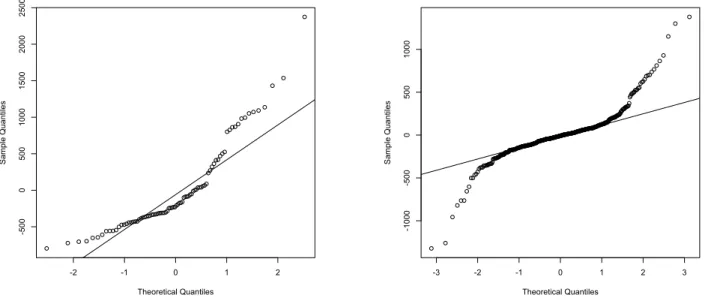
Before presenting the results from this simulation study we would like to show some model and spatial diagnostics. Figure 1 shows normal probability plots of level 1 and level 2 residuals obtained by fitting a two-level (level 1 is the lake and level 2 is the HUC) mixed model to the synthetic population data. The normal probability plots indicate that the Gaussian assumptions of the mixed model are not met. Hence, the use of a model that relaxes these assumptions, such as the M-quantile model, can be justified in this case. In order to detect whether there is spatial autocorrelation in the EMAP data we computed the Moran’sI coefficient. The standardized Moran’sI is analogous to the correlation coefficient, and its values range from 1 (strong positive spatial autocorrelation) to -1 (strong negative spatial autocorrelation). For the EMAP data Moran’sI = 0.61
indicating a positive spatial correlation. There is also evidence of a non-stationary process. In particular, using an ANOVA test proposed by Brundson et al. (1999) we rejected the null hypothesis of stationarity of the model parameters. Based on the spatial diagnostics we expect that incorporating the spatial information in small area estimation may lead to gains in efficiency. The results set out in Tables 1 and 2 show the across areas and simulations distribution of relative bias and relative root mean squared error for in sample and out of sample areas respectively. Focusing first on Table 1 we note that all small area predictors based on the different variants of the M-quantile GWR model have significantly lower relative bias than theEBLUP SEBLUP, andNPEBLUPpredictors with theMQGWRpredictor performing best. Examining the performance in terms of relative root mean squared error we note that the small area predictors that account for the spatial structure of the data have on average smaller root mean squared errors with theNPEBLUP,SEBLUPandMQGWRpredictors performing best. The increased relative root mean squared error of theMQGWRpredictors can be explained by the bias variance trade off associated with the use of robust methods. That is, although by using the M-quantile GWR model we reduce the bias of the point estimates, theMQGWRpredictors have higher variability. One way of potentially tackling this problem is by making the M-quantile GWR model less robust for example by setting in the Huber influence function c > 1.345. These results also show that
-2 -1 0 1 2 -500 0 500 1000 1500 2000 2500 Theoretical Quantiles Sample Quantiles -3 -2 -1 0 1 2 3 -1000 -500 0 500 1000 Theoretical Quantiles Sample Quantiles
Figure 1: Normal probability plots of level 2 (left) and level 1 residuals (right) derived by fitting a two level linear mixed model to the synthetic population data.
there is a substantial number of in-sample HUCs where theMQGWRpredictor has lower RRMSE than theNPEBLUPand
SEBLUPpredictors.
Focusing now on Table 2 we note that for out of sample areasNPMQandMQGWR-based small area predictors have lower relative biases and lower root mean squared errors than theEBLUP,NPEBLUPandSEBLUPpredictors. This supports our original hypothesis that the M-quantile GWR model offers a straightforward approach for improving synthetic estimation for out of sample areas. The performance of theSEBLUPpredictor in this case may be surprising. However, we should bear in mind that for out of sample areas we use a syntheticSEBLUP. A more elaborate method for out of sample areas under the SAR model has been proposed by Saei & Chambers (2005).
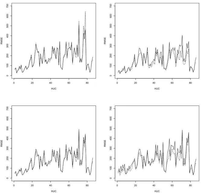
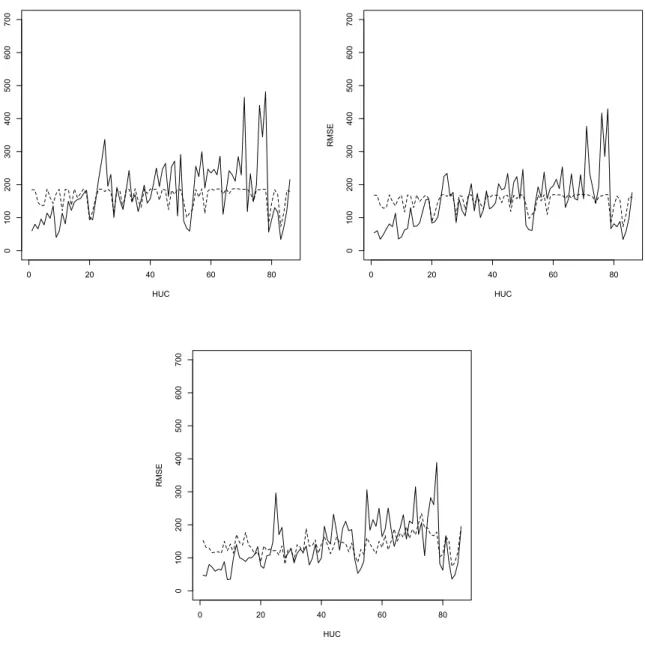
Figures 2 and 3 show how the different mean squared estimators track the true mean squared error of the different predictors. Here we see that mean squared estimator described in Tzavidis et al. (2008), and its version (18) under the M-quantile GWR model, perform well in terms of tracking the true mean squared error of the M-quantile small area predictors. Finally, we see that the Prasad-Rao type MSE estimators of theEBLUP,NPEBLUPandSEBLUPperform poorly in this application as far as tracking the area-specific mean squared error is concerned. This phenomenon has been also reported in other design-based studies (Chambers et al., 2008). As the model diagnostics have already demonstrated, for this data the Gaussian assumptions of the mixed model are not satisfied. This provides a further explanation for the performance of the Prasad-Rao type mean squared estimators in this case.
6 Conclusions
In this paper we contrasted different approaches for borrowing strength over space in small area estimation using parametric, semiparametric and nonparametric small area models. Our results show that incorporating the spatial information in small area estimation can lead to significant gains in the efficiency of the small area estimates. The penalized splines model appears to be a useful tool when the functional form of the relationship between the variable of interest and the covariates is left unspecified and the data are characterized by complex patterns of spatial dependency. An advantage of the M-quantile GWR-based estimators is that they perform better than theSEBLUP,NPEBLUPestimator for estimating parameters for out of sample areas. One approach for potentially improving the performance of theSEBLUPestimator for out of sample areas is to use the Saei & Chambers (2005) SAR mixed model. A further advantage of the M-quantile GWR model is that it allows for outlier robust inference. As we illustrated in section 5, the violation of the assumptions of the mixed model may lead to substantial bias in the small area estimates derived with theEBLUP SEBLUPandNPEBLUPpredictors. The violation of the assumptions of the mixed model also affects the performance of the Prasad-Rao type mean squared error estimators. On the other hand, the use of a robust approach to small area estimation tackles the problem of bias though at the expense of higher variability. Approaches to balancing this bias variance trade off were briefly described in section 5. In a recent paper Sinha & Rao (2008) proposed the use of a robust mixed model for small area estimation. The robust mixed model can be directly compared to the M-quantile
Table 1: Design-based simulation results using the EMAP data. Results show the distribution of Relative Bias (RB) and Relative Root Mean Squared Error (RRMSE) over areas and simulations for the 86 sampled HUCs.
Percentile of across area distribution Predictor 10 25 Mean 50 75 90 Relative Bias (%) EBLUP -9.51 0.39 -12.55 10.79 21.43 36.85 SEBLUP -10.59 -5.12 5.27 2.50 12.33 27.53 MQ -4.08 -2.34 -0.83 -0.42 1.32 2.39 MQGWR -3.76 -1.69 0.22 0.06 1.79 4.66 MQGWR-LI -4.59 -2.24 -0.78 -0.71 0.85 2.58 NPEBLUP -10.75 -1.23 12.19 10.45 23.70 37.17 NPMQ -7.08 -1.53 6.42 7.19 13.26 18.48 RRMSE (%) EBLUP 21.33 23.95 38.05 35.18 49.49 60.09 SEBLUP 16.13 20.46 31.50 29.01 38.61 52.95 MQ 19.66 25.81 39.45 35.49 49.71 67.65 MQGWR 16.38 21.49 33.61 29.84 43.22 55.24 MQGWR-LI 18.07 23.86 35.64 34.03 46.22 56.82 NPEBLUP 16.53 19.22 30.77 26.09 41.73 49.10 NPMQ 20.97 27.45 40.03 39.15 48.45 61.87
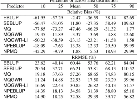
Table 2: Design-based simulation results using the EMAP data. Results show the distribution of Relative Bias (RB) and Relative Root Mean Squared Error (RRMSE) over areas and simulations for the 27 out of sample HUCs.
Percentile of across area distribution
Predictor 10 25 Mean 50 75 90 Relative Bias (%) EBLUP -61.95 -57.29 -2.47 -36.59 38.14 82.69 SEBLUP -56.47 -51.05 11.80 -27.35 58.49 109.63 MQ -77.85 -73.27 -47.46 -66.29 -31.32 1.77 MQGWR -19.35 -11.89 -3.37 -3.69 4.88 12.60 MQGWR-LI -50.23 -38.59 -23.13 -23.21 -11.58 1.58 NPEBLUP -18.09 -7.63 13.38 12.33 29.50 59.99 NPMQ -42.29 -9.79 1.88 5.53 18.93 29.99 RRMSE (%) EBLUP 23.62 40.14 60.44 53.76 62.21 84.04 SEBLUP 20.54 37.71 66.21 53.81 68.13 110.52 MQ 19.18 37.63 57.26 68.65 74.83 80.15 MQGWR 11.24 14.88 22.93 17.50 23.29 39.96 MQGWR-LI 16.69 22.43 30.85 26.82 40.13 51.57 NPEBLUP 14.39 18.13 34.58 31.39 38.80 65.10 NPMQ 14.90 18.25 32.58 29.39 39.77 56.82
0 20 40 60 80 0 100 200 300 400 500 600 700 HUC RMSE 0 20 40 60 80 0 100 200 300 400 500 600 700 HUC RMSE 0 20 40 60 80 0 100 200 300 400 500 600 700 HUC RMSE 0 20 40 60 80 0 100 200 300 400 500 600 700 HUC RMSE
Figure 2: HUC-specific values of actual design-based RMSE (solid line) and average estimated RMSE (dashed line). Top left is the approximation to the RMSE of theMQ predictor. Top right is the approximation to the RMSE of theMQGWRpredictor. Bottom left is the approximation to the RMSE of the MQGWR-LI predictor and bottom right is the approximation to the RMSE of theNPMQ (ag.sp) predictor. Estimates of the RMSE under the different models are obtained using the mean squared error estimator suggested by Chambers et al. (2008).
0 20 40 60 80 0 100 200 300 400 500 600 700 HUC RMSE 0 20 40 60 80 0 100 200 300 400 500 600 700 HUC RMSE 0 20 40 60 80 0 100 200 300 400 500 600 700 HUC RMSE
Figure 3: HUC-specific values of actual design-based RMSE (solid line) and average estimated RMSE (dashed line). Top left is the Prasad & Rao (1990) approximation to the RMSE of theEBLUPpredictor. Top right is the approximation to the RMSE of theSEBLUPpredictor using the RMSE estimator of section 2.1. Bottom left is the approximation to the RMSE of the
small area model and we currently working on comparing the two models. Extending further the outlier robust mixed model into an outlier robust SAR mixed model will further improve the collection of small area estimation tools.
References
ANSELIN, L. (1988).Spatial Econometrics. Methods and Models. Boston: Kluwer Academic Publishers.
BANERJEE, S., CARLIN, B. & GELFAND, A. (2004). Hierarchical Modeling and Analysis for Spatial Data. New York: Chapman and Hall.
BATTESE, G. E., HARTER, R.M. & FULLER, W.A.(1988). An error-components model for prediction of county crop areas using survey and satellite data. Journal of the American Statistical Association83, 28-36.
BRUNDSON, C., FOTHERINGHAM, A.S. & CHARLTON, M.(1996). Geographically weighted regression: a method for ex-ploring spatial nonstationarity. Geographical Analysis28, 281-298.
BRUNDSON, C., FOTHERINGHAM, A.S. & CHARLTON, M.(1999). Some notes on parametric significance tests for geograph-ically weighted regression. Journal of Regional Science39, 497-524.
CHAMBERS, R. & DUNSTAN, R. (1986). Estimating distribution function from survey data.Biometrika73, 597-604. CHAMBERS, R. & TZAVIDIS, N. (2006). M-quantile Models for Small Area Estimation. Biometrika93, 255-268.
CHAMBERS, R., TZAVIDIS, N. & CHANDRA, H. (2008). On robust mean squared error estimation for linear predictors for domains. [paper submitted for publication, available upon request]
CRESSIE, N. (1993).Statistics for Spatial Data. New York: John Wiley & Sons.
DAS, K., JIANG, J. & RAO, J.N.K. (2004). Mean squared error of empirical predictor.Ann. Statist.32, 818-840.
DATTA, G.S. & LAHIRI, P. (2000). A Unified Measure of Uncertainty of Estimates for Best Linear Unbiased Predictors in Small Area Estimation Problem. Statistica Sinica10, 613–627.
FOTHERINGHAM, A.S., BRUNDSON, C. & CHARLTON, M.(1996). Two techniques for exploring non-stationarity in geo-graphical data.Geographical Systems4, 59-82.
FOTHERINGHAM, A.S., BRUNDSON, C. & CHARLTON, M.(1996). Geographically Weighted Regression West Sussex: John Wiley & Sons.
KACKAR, R. & HARVILLE, D. (1984). Approximations for standard errors of estimators for fixed and random effects in mixed models.Journal of the American Statistical Association79, 853–862.
KAUFMAN, L. & ROUSSEEUW, P. (1990). Finding Groups in Data: An Introduction to Cluster Analysis. New York: Wiley. HENDERSON, C. (1975). Best linear unbiased estimation and prediction under a selection model.Biometrics31, 423–447. HARVILLE, D.A. & JESKE, D.R. (1992). Mean squared error of estimation or prediction under a general linear model.Journal
of the American Statistical Association87, 724–731.
LARSEN, D. P., KINCAID, T. M., JACOBS, S. E. & URQUHART, N. S.(2001). Designs for evaluating local and regional scale trends.Bioscience51, 1049-1058.
LONGFORD, N.T. (2007). On standard errors of model-based small area estimators. Survey Methodology33, 69–79.
NYCHKA, D. & SALTZMAN, N. (1998). Design of air quality monitoring networks. InNychka, Douglas, Piegorsch, Walter W. and Cox, Lawrence H. (eds), Case studies in environmental statistics
OPSOMER, J. D. CLAESKENS, G., RANALLI, M. G., KAUERMANN, G. & BREIDT, F. J.(2008). Nonparametric small area estimation using penalized spline regression.Royal Statistical Society, Series B70, 265–283.
PETRUCCI, A. & SALVATI, N. (2006). Small area estimation for spatial correlation in watershed erosion assessment. Journal of Agricultural, Biological and Environmental Statistics11, 169–182.
PRASAD, N. & RAO, J. (1990). The estimation of the mean squared error of small-area estimators. Journal of the American Statistical Association85, 163–171.
PRATESI, M. & SALVATI, N. (2007). Small area estimation: the EBLUP estimator based on spatially correlated random area
effects. Statistical Methods & Applications17, 113–141.
PRATESI, M., RANALLI, M. G.& SALVATI, N. (2008). Semiparametric M-quantile regression for estimating the proportion of acidic lakes in 8-digit HUCs of the Northeastern US.Environmetrics19, 687–701.
RAO, J.N.K., KOVAR, J.G. & MANTEL, H.J. (1990). On Estimating Distribution Functions and Quantiles from Survey Data Using Auxiliary Information.Biometrika77, 365-375.
RAO, J. N. K. (2003).Small Area Estimation. London: Wiley.
ROYALL, R.M. & CUMBERLAND, W.G. (1978). Variance estimation in finite population sampling. Journal of the American Statistical Association73, 351–358.
RUPPERT, D., WAND, M. P.& CARROLL, R.(2003).Semiparametric Regression. Cambridge: Cam- bridge University Press. SAEI, A. & CHAMBERS, R. (2005). Empirical Best Linear Unbiased Prediction for Out of Sample Areas. Working Paper
M05/03, Southampton Statistical Sciences Research Institute, University of Southampton.
SALVATI, N., TZAVIDIS, N., PRATESI, M. & CHAMBERS, R. (2008). Small Area Estimation Via M-quantile Geographically Weighted Regression.[paper submitted for publication, available upon request]
SALVATI, N., RANALLI, M.G. & PRATESI, M. (2008a). Nonparametric M-quantile Regression using Penalized Splines in Small Area Estimation [paper submitted for publication, available upon request]
SINGH, B., SHUKLA, G. & KUNDU, D. (2005). Spatio-temporal models in small area estimation. Survey Methodology31, 183–195.
SINHA, S.K. & RAO, J.N.K. (2008). Robust Small Area Estimation. [paper submitted for publication]
TZAVIDIS, N., MARCHETTI, S. & CHAMBERS, R. (2008). Robust prediction of small area means and distributions. [paper submitted for publication, available upon request]
YU, D.L. & WU, C. (2004). Understanding population segregation from Landsat ETM+imagery: a geographically weighted regression approach. GISience and Remote Sensing41, 145–164.
ZIMMERMAN, D.L. & CRESSIE, N. (1992). Mean squared prediction error in the spatial linear model with estimated covari-ance parameters. Ann. Inst. Stat. Math.44, 27–43.