Global Factor Returns

UC Irvine

UC Irvine Electronic Theses and Dissertations

Title

Global Factor Returns

Permalink

https://escholarship.org/uc/item/3z888825

Author

Viswanathan, Vivek

Publication Date

2019

Peer reviewed|Thesis/dissertation

eScholarship.org

Powered by the California Digital Library

i

UNIVERSITY OF CALIFORNIA,

IRVINE

Global Factor Returns

DISSERTATION

submitted in partial satisfaction of the requirements

for the degree of

DOCTOR OF PHILOSOPHY

in Finance

by

Vivek Viswanathan

Dissertation Committee:

Professor Philippe Jorion, Chair

Professor Zheng Sun

Assistant Professor David C. Yang

ii

ii

DEDICATION

To

Max

Ginger

Mocha

Latte

Java

Dia

Meena

Titan

Moth

iii

TABLE OF CONTENTS

ACKNOWLEDGMENTS v

CURRICULUM VITAE vi

ABSTRACT OF THE DISSERTATION vii

CHAPTER 1: GLOBAL FACTOR RETURNS 1

1.2 Factor Returns 7

1.2.1 Methodology 7

1.2.2 Factor Returns Results Overview 8

1.2.3 Global 9

1.2.4 United States 10

1.2.5 Developed ex US 10

1.2.6 Emerging Markets 11

1.2.7 Factor Equal-Weights 11

1.2.8 Alpha Against United States 14

1.2.9 Post-Sample Returns 14

1.2.10 Covariances vs. Characteristics 15

1.2.11 Long vs. Short Returns 16

1.2.11 Factor Volatilities 17

1.3 Determining Which Factors Deliver Excess Return 17

1.4 Indicators of market efficiency 19

1.5 Are markets becoming more efficient? 20

1.6 Transaction Costs 21

1.5 Conclusion 22

1.7 References 23

CHAPTER 2: HIGH-DIMENSION FACTOR RETURNS 25

2.1 Data 27

2.2 The Capital Asset Pricing Model (CAPM) 27

2.3 Collapsing the Factor Space 28

2.3.1 Fama French 3-Factor Model (FF3) 29

2.3.2 Carhart 4-Factor Model 29

2.3.3 Fama French 5-Factor Model (FF5) 30

2.3.4 Novy-Marx 5-Factor Model (NM) 30

2.3.5 Hou, Xue, and Zhang 4-Factor Model (HXZ) 31

2.3.6 Stambaugh and Yuan 4-Factor Model (SY4) 32

2.3.7 Daniel, Hirshleifer, and Sun 3-Factor Model (DHS) 32

iv

2.3.9 Summary 34

2.4 Principal Component Analysis 35

2.5 Conclusion 36

2.6 References 37

CHAPTER 3: MACHINE LEARNING IN GLOBAL EQUITY MARKETS 39

3.1 Data 40 3.2 Methodology 41 3.2.1 Data Pre-Processing 41 3.2.2 Linear Regression 42 3.2.3 Ridge Regression 43 3.2.4 Gradient Boosting 43 3.2.5 Random Forest 44

3.2.6 Calibration and Prediction 44

3.2.7 Regularization Parameters 46

3.2.8 Ensemble Forecast 46

3.2.9 Portfolio Construction 47

3.3 Results 47

3.3.1 Linear Regression Results 47

3.3.2 Machine Learning Models 49

3.4 Conclusion 51

3.5 References 52

v

ACKNOWLEDGMENTS

I want to thank Professor Philippe Jorion, Professor David Hirshleifer, Professor David Yang, Professor Zheng Sun, and Professor Ivan Jeliazkov for their deep insights into the theory, structure, and empirics of this thesis. Their contributions have both enlightened me and greatly improved this document.

vi

CURRICULUM VITAE

Vivek Viswanathan

2005

B.A. in Economics, University of Chicago

2006

Research Associate, Center for Microfinance, Chennai, India

2007-16

Senior Researcher, Vice President, Research Affiliates, Newport Beach, CA

2009

Masters in Financial Engineering, University of California, Los Angeles, CA

2016-

Global Head of Research, Rayliant Global Advisors, Irvine, CA

2019

Ph.D. in Finance, University of California, Irvine, CA

FIELD OF STUDY

Cross-sectional equity anomalies

PUBLICATIONS

“Two Determinants of Lifecycle Investment Success,” The Journal of Retirement, 2015,

Coauthors: Jason Hsu, Jonathan Treussard, Lillian Wu, Published in (2015)

“A Framework for Assessing Factors and Implementing Smart Beta Strategies,” The Journal of

Index Investing, Summer 2015, Co:authors: Jason Hsu, Vitali Kalesnik

“Momentum and Mean-Reversion in Commodity Spot and Futures Markets,” Journal of

Commodity Markets, September 2016, Coauthor: Denis Chaves

“The Low Volatility Anomaly and the Preference for Gambling,” Risk-Based and Factor

Investing, November 2015, Coauthor: Jason Hsu

“Anomalies in Chinese A-Shares,” Journal of Portfolio Management, Summer 2018, Coauthors:

Jason Hsu, Chenhui Wang, Phillip Wool

“Outperformance through Investing in ESG in Need,” Journal of Index Investing, Summer 2018,

Coauthors: Jason Hsu, Xiaoyang Liu, Keren Shen, Yanxiang Zhao

“Illiquidity and Factor Returns,” Journal of Investment Management, October 2018, Coauthor:

Jason Hsu.

vii

ABSTRACT OF THE DISSERTATION

Global Factor Returns

By

Vivek Viswanathan

Doctor of Philosophy in Finance

University of California, Irvine, 2019

Professor Philippe Jorion, Chair

The 86 of 97 McLean and Pontiff (2016) factors that can be readily tested internationally deliver

higher returns in Developed ex US and yet higher returns in Emerging Markets than in the United

States. An equally weighted portfolio of these factors is highly significant in each region and such

portfolios in Developed ex US and Emerging Markets earn a significant alpha on their US

counterpart. In no region are these factors adequately explained by current models that attempt to

explain factor excess returns. These factors are driven by the underlying characteristics as opposed

to loadings on risk factors demonstrating that these factors are anomalies, not priced risks.

However, there is some evidence that the premia on these anomalies and the characteristics’ ability

to predict return are declining over time.

1

CHAPTER 1: GLOBAL FACTOR RETURNS

The same factors that have been tested in the United States deliver high premia in

developed markets excluding the United States (DevxUS) and yet higher premia in emerging

markets (EM). This suggests that on average, the decline in factor premia in the United States is

primarily a result of greater efficiency and not pure data snooping. In addition, it demonstrates that

the behavioral inefficiencies in the United States are not specific to culture, economic structure, or

regulations but instead reflect apparent failures of human rationality or attention in understanding

universal economic phenomena.

I examine the robustness of factors by testing 86 of the 97 McLean and Pontiff (2016)

factors across global markets and find that while most factors are insignificant in their own right,

an equally weighted portfolio of factors is significant in each region and this portfolio is more

significant in DevxUS than in the United States and more significant in EM than in DevxUS.

Similar to Lu, Stambaugh, and Yuan (2018) for a smaller subset of factors and Jacobs and Müller

(2019), I find that these anomalies are globally robust. Moreover, more factors are individually

significant in EM than in DevxUS and in DevxUS than in the US. In addition, factors are more

often significant and earn higher returns in small stocks than large stocks. Given the lower attention

paid to and lower liquidity in smaller and emerging market stocks, this may be a function of limited

attention or limits to arbitrage due to lower liquidity.

The factor performance in DevxUS and EM is not a mere result of correlation with US

factors. An equally weighted portfolio of factors in DevxUS and an equally weighted portfolio of

factors in EM each earns an alpha significant at a 0.01 level on the US equally weighted portfolio

of factors.

The returns of these 86 factors are driven entirely by characteristics, not covariances. In

other words, they are behavioral anomalies, not risk factors. Few factors built from factor loadings

as opposed to characteristics are significant, whereas numerous factors built from characteristics

are significant. An equally weighted portfolio of factors based on characteristics subsumes an

equally weighted portfolio of factors based on covariances.

Moreover, the fact that 1) 17 principal components are needed to explain 90% of the

variance of factor returns globally and 2) which factors deliver positive excess returns in any given

period is time varying suggests that collapsing many factors into few may not be possible. Further,

predictive regressions of returns demonstrate that the characteristics that predict return vary from

period to period. All told, this suggests factors are robust globally and not subsumable by fewer

factors.

As Harvey, Liu, and Zhu (2016) note, over a hundred factors have been discovered in the

United States, but most no longer work and many never even worked in the sample in which they

were originally investigated. This implies a collective data snooping by the academic and

practitioner finance community. They suggest increasing the required t-stat to 3 for rejecting the

null of 0 factor excess returns at a 0.05 level. However, it’s not clear that such a high t-stat is

actually warranted since many of the equity results they examined are time series claims, not

cross-sectional ones. Moreover, I avoid this high t-stat requirement by equally weighting all factors into

one portfolio in regions outside of the original test and post-sample, effectively collapsing the

multiplicity of factors into one. However, the t-stats for the individual factors should be viewed

with the suitable skepticism.

McLean and Pontiff (2016) examine 97 factor returns and find that t-stats have fallen in

half post-sample. Such a result can either be a result of arbitrage as practitioners implemented

these anomalies or data mining as the high in-sample t-stats collapsed. The results in this paper

suggest the decline is due to arbitrage at least in part.

Instead of looking post-sample, Linnainmaa and Roberts (2016) examine factor returns in

a prior sample before the Compustat coverage period using Moody's Industrial and Railroad

manuals. The pre-sample returns demonstrate that the factor returns were not robust. However, the

United States may be sufficiently different between 1947 and 1965 that the same factors may not

work. Of course, the exact same argument can be leveled against using international stock returns.

Lastly, Novy-Marx (2016) suggests that t-stats that account for multiple hypotheses would

dismiss most false anomalies as data mining. He specifically targets composite factors such as

Piotroski F-Score or Mohanram G-Score which contain multiple metrics in their construction. If a

researcher has the choice to flip each element of a composite score to be positively sorted or

negatively sorted, then even if each element is insignificant, the combination can be extremely

highly significant. This fact remains true irrespective of the results presented here.

Instead of approaching the analysis of factors by looking pre- and post-sample, I choose to

look outside the United States. Such an approach is necessarily riddled with data issues that prevent

proper testing of all 97 McLean and Pontiff factors. In addition, testing the robustness of anomalies

internationally does not have the same clean test of looking pre- and post-sample, since factors are

correlated across regions.

One can rationally argue that investors behave differently in different regions and thus,

different anomalies will naturally arise. This is likely true. Indeed, Arkes, Hirshleifer, Jiang, and

Lim (2008) find cultural differences in reference point adaptation which should affect the

momentum anomaly. Weber and Hsee (1998) and Hsee and Weber (1999) show that Chinese

investors are more risk-seeking than American ones, which would affect the strength of the

volatility, beta, and residual variance anomalies. Ji, Nisbett, and Su (2001) find that Chinese

students are more likely to believe that trends will continue than their American counterparts,

which would affect momentum and reversal anomalies.

Some markets such as those in Taiwan are far more heavily dominated with retail investors

than in the United States where most trading is done by institutions and increasingly by algorithms.

Some countries have stricter accounting rules than others. Some demonstrate far greater earnings

management than others. For example, most emerging markets show a stronger jump around 0%

in a return on equity histogram than in the United States. However, if anomalies reflect something

fundamental about human behavior whether driven by inattention, underreaction, overreaction, or

risk preferences, then we would expect the anomalies to persist globally. In other words, if factors

were not robust globally, it would not inherently suggest that they do not work in the United States.

However, the fact that they do work globally suggests that they reflect something more

fundamental as opposed to something specific to the United States and certainly refutes the notion

that the historical literature on factors is a mere result of data-mining. This result and conclusion

are the same of that of Jacobs and Müller (2019).

A second objection to using international data as a robustness test is that the returns are

correlated with US data. As discussed, while correlated, an equally weighted portfolio of EM or

DevxUS factors earns a significant positive alpha on an equally weighted portfolio of US factors,

suggesting that an orthogonal component of the factors earns excess return.

Unlike many papers, I report large capitalization and small capitalization factor returns

separately. The returns of large capitalization factors are generally lower than those of small

capitalization factors similar to the results found in Hsu and Viswanathan (2018). The

methodology involved in Fama and French (1992) and nearly every other paper on factors of

averaging large and small cap factor returns thus results in an exaggeration of the statistical

significance of factors or at least an exaggeration of what can be practically earned by an investor

of any reasonable size.

1.1 Data

I use Worldscope data for financial data and Datastream for market data. I match the

adjustments that Compustat makes to ensure that the signals are comparably calculated. I choose

Worldscope for financial data over other sources like Thomson Financial because Worldscope

implements a litany of data adjustments to ensure comparability across countries.

I match Worldscope with Datastream through a matching table between DS Company

Code and Worldscope ID, similar to CRSP / Compustat Merged. Country inclusion and

classification into developed and emerging are based on MSCI. All non-OTC exchanges are

included in each country. Country classification is based on country of domicile for the primary

operating business of the firm as opposed to the exchange listing. Results are not sensitive to basing

country designation on exchange.

A currency change in Brazil in the early 1990s results in a large bias in market

capitalizations in the subsequent 4 years. Using other sources of exchange rates from Bloomberg

fail to fully remedy this problem, so I start samples in July 1995.

I compare total returns and price returns for individual stocks. If total return exceeds price

return in a day by more than 500%, then the total return is set to equal the price return. Presumably,

no firm would pay out such a high percentage of its value as a dividend in one day, so such an

observation is likely a data error. Bloomberg and CRSP data verify that such data are likely

erroneous. If price returns ever exceed total returns, then price returns are set to total return. Lastly,

if return exceeds 2500% or is less than -96% in a day that return is set to 0. These values are chosen

for symmetry in effect on geometric return. Again, the presumption is that returns above 2500%

or below -96% are erroneous, which I verify in the US using data from CRSP and Bloomberg. If

any total or price return data are missing, the returns are set to 0.

I use the market capitalization breakpoints for the NYSE from French Data Library. Only

stocks above the 20th percentile are included (all but tiny). The rationale for the exclusion of such

stocks are the sheer number of such stocks and the frequency of outlier returns among such stocks.

I use NYSE breakpoints, since the inclusion of new exchanges in the database affects the

distribution of market capitalizations dramatically. Market capitalizations in USD come from

Datastream.

Certain factors from McLean and Pontiff (2016) are not computed due to lack of data:

Change in Recommendation, which requires analyst recommendations; Debt Issuance, which

requires debt issuance from the cash flow statement; Exchange Switch; IPO + Age, which requires

the initial public offering of the company; Mergers; Ratings Downgrades; SEOs; Spinoffs;

Advertising/MV because advertising is not broken out as a separate line item in Worldscope;

Marketing/MV because marketing is not broken out as a separate line item in Worldscope; and

G-Index, since it requires specific information about corporate governance.

While I do not compute IPO + Age, I do compute the IPO factor and Age factor individually

by using the months since appearance in the database as a proxy. In order to prevent issues arising

from new exchanges being added to Datastream causing a false positive for an IPO, no IPO or Age

signals were calculated for any stocks that were added due to a new exchange being added to the

database.

1.2 Factor Returns

1.2.1 Methodology

I test all anomalies for which data are available in McLean and Pontiff (2016). I choose

McLean and Pontiff (2016) as the baseline because the anomalies are tractable and categorized. I

use the categories merely as a tool for organization. The 86 anomalies tested are shown in Table 1

along with their corresponding citations.

As discussed previously, I remove tiny stocks from our sample as defined by below 20th

percentile NYSE market capitalization. Next, I group stocks into large and small buckets based on

total market capitalization with the NYSE 60th percentile denoting the breakpoint between large

and small. I use 60th percentile as the demarcation point between large and small because the

removal of tiny stocks shifts the market capitalization midpoint.

I sort stocks based on the given characteristic in the direction such that the long portfolio

is expected to generate positive excess returns over the short portfolio. I base the sorting direction

on papers that initially discovered the anomalies cited in McLean and Pontiff (2016). Unlike

Jacobs and Muller (2019) I report the returns, volatilities, and t-stats of the individual factors

including within large cap stocks, within small cap stocks, and the average of the large and small

factors returns. The separation of the results is meant to elucidate the difference in returns of factors

among large and small stocks. I average the large and small returns to produce the factor factors.

I also calculate the equal-weighted portfolio of all factor returns in a given region in the

large, small, and average portfolios. The equally weighted portfolio of all factor returns represents

the combined significance of all factors and is probably the cleanest determinant of whether factors

as whole generate excess returns even if such a test tells us nothing about which factors generate

excess return. Any given factor in a long list of factors can generate positive excess return. The

average of all factor returns in an out-of-sample test represents the ability of these factors to

collectively predict return without the in-sample, outlier, or autocorrelated standard error problems

that would occur with a regression.

For the purposes of the factor results, we construct size exactly as the other factors—top

30% minus bottom 30% within large and small. However, for the purposes of the explanatory

regressions such as the Fama-French 3-Factor model, we construct size as top 40% minus the 20

to 60

percentile.

Unlike Jacobs and Muller (2019), I remove tiny stocks which are largely untradable but

can make up a disproportionate component of stocks in the long and short portfolio as they are

more likely to have extreme financial and market behavior. In addition, I aggregate stocks into the

regions of US, DevxUS, and EM, which permits an interrogation of the orthogonal component of

excess returns from EM with respect to the other regions.

1.2.2 Factor Returns Results Overview

Table 2 shows the number of significant factors in each region and size category. In

general, factors in large capitalization stocks do not show particularly strong significance. At a

0.05 level, global large has 10 significant factors, US large 2 significant factors, DevxUS large 6

significant factors, and EM large 4 significant factors. Small cap stocks show far more significant

factors across regions with 27 factors significant in global small, 8 significant in the US small, 23

significant in DevxUS small, and 36 in EM small. These small stocks generate an outsized

influence on the significance of the average of factor portfolios within large and small. When one

averages the large and small factors, 20 are significant in global, 5 in the US, 15 in DevxUS, and

19 in EM.

In general, the higher frequency of significant factors among small stocks is consistent with

investors arbitraging these factors in large stocks but less so in smaller, more illiquid stocks. The

outperformance among small stocks suggests that the factors are more likely to persist, given the

lower liquidity of such stocks.

Factors are rarely negatively significant. Among the average of large and small factors, 2

are negatively significant at a 0.05 level in global, zero in the US, 3 in DevxUS, and zero in EM.

This asymmetry suggests that the factors are more likely to deliver excess return than not but is

hardly definitive given that many of the factors are highly correlated. I tackle this issue more

rigorously when looking at equally weighted factors.

1.2.3 Global

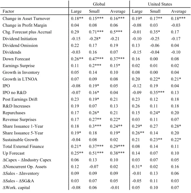
Table 3 shows factor returns within each region and within large and small. Twenty factor

returns are significantly positive at a 0.05 level or better among the average of large and small

factor returns: change in asset turnover, change in forecast plus accruals, down forecast, one-year

share issuance, total external finance, up forecast, coskewness, industry momentum, cash flow /

MV, earnings-to-price, enterprise multiple, accruals, asset turnover, gross profitability, G-Score,

F-Score, M/B and accruals, percent operating accruals, profitability, and ROE. Only two factors,

bid-ask spread and cash flow variance, are negatively significant at a 0.05 level. Why bid-ask

spread fails is not clear but is likely in part due to the sheer number of factors that are being tested—

if enough tests are run, some are likely to show negative significance regardless of their actual

expected return. Alternatively, it may simply be that illiquidity is not priced by the market. Brennan

and Subrahmanyam (1996), Spiegel and Wang (2005), Ben-Rephael, Kadan, and Wohl (2015),

and Lou and Shu (2014) find weak or no evidence for an illiquidity premium. Firms with low cash

flow variance tend to have low betas and to be growth firms, so the factor does not earn a

significantly negative CAPM alpha or a significant Fama-French 3-Factor alpha.

1.2.4 United States

Factor returns in the United States during this period are weaker than those globally. Given

that we are using a period between 1995 to 2018, our results are consistent with McLean and

Pontiff (2016). That is, factors are relatively weak during this time period in the United States.

A mere 5 factors are positively significant at a 0.05 level when looking at the average of

large and small: change in asset turnover, Mohanram G-Score, leverage, M/B and accruals, and

percent operating accrual. Such a miniscule number of significant factors is consistent with none

of the factors working in the US and the significant ones being the result of imprecise estimation

on a finite sample. Two factors are significant in the large cap space: 5-year share issuance and

NOA. Among small cap stocks, 8 of 86 factors are significantly positive at a 0.05 level, a mere 9%

of tested factors.

The weakness in the US is telling. It is no wonder that numerous publications have claimed

that the factors are likely a result of data mining and that markets are far more efficient than the

sheer number of published factors would suggest. I will show in the Factor Equal-Weights

subsection that there are significant returns to be found in this data and in the Collapsing the Factor

Weights section that there are significant alphas in numerous factors.

No factors are negatively significant in the US.

1.2.5 Developed ex US

DevxUS shows greater factor significance than in the US. Fifteen factors are significant

among the average of the large and small factor returns at a 0.05 level: change in forecast plus

accruals, down forecast, total external finance, up forecast, 52-week high, coskewness, industry

momentum, cash flow / MV, dividend yield, earnings-to-price, enterprise multiple, F-Score, profit

margin, profitability, and ROE. Three factors are negatively significant: bid-ask spread,

Herfindahl, and tax. As globally, bid-ask spread is seemingly priced in the opposite direction. Lev

and Nissim (2004) find that Tax, the ratio of tax-to-book income, predicts subsequent 5-year

earnings growth and suggested that investors are becoming more aware of this relationship. At

least in DevxUS, either this economic relationship has flipped or investors are now overreactingg

to the relationship.

Six factors are positively significant in the large cap space while 23 are significant in the

small cap space.

1.2.6 Emerging Markets

Within EM, 19 factors are significant at a 0.05 level when looking at the average of large

and small cap returns: change in asset turnover, change in forecast plus accruals, down forecast,

post earnings drift, R&D increases, up forecast, coskewness, long-term reversal,

momentum-reversal, book-to-market, cash flow / MV, dividend yield, earnings-to-price, enterprise multiple,

organizational capital, sales / price, asset turnover, operating leverage, and profitability. No factors

are negatively significant in emerging markets for the average of large and small factors.

Within the large cap space, 4 factors are positively significant at a 0.05 level or better,

while in the small cap, 36 are positively significant.

1.2.7 Factor Equal-Weights

A natural issue with the above results is that I am testing numerous hypotheses but still

merely demanding a 1.96 t-stat threshold that would be used for a single hypothesis test. But while

any individual factor cannot be said to be significant at a 5% level with a t-stat of 1.96 given the

many hypotheses that are being tested, an equally weighted portfolio of factors is not subject to

this issue. This same approach was used by Jacobs and Muller (2019). Testing equally weighted

factor portfolios involves 12 correlated hypotheses for each of the four tested regions in large,

small, and the average as opposed to the 1,020 correlated hypotheses involved in testing 86 factors

in four tested regions in large, small, and the average of the two.

This averaging approach also sidesteps the Novy-Marx (2016) objection about testing

multiple signals. This does not involve choosing the factors that have done well in-sample by

flipping the signs of factors if they perform negatively. I simply implement all factors as they are

implemented in their original research in the United States and average them. While this suffers

from publication bias in the United States for all factors published after July 1995, the problem is

far less pronounced outside the United States.

Moreover, this approach handles the issue of the low signal-to-noise ratio for any given

factor. If all factors are equally weighted, the collective signal remains while the individual noise

cancels out.

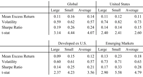
Table 4 shows the results of this analysis and demonstrates that the factors are significant

in every region, are more significant in small cap stocks than large cap stocks, and among average

of large and small factors, are more significant in EM than in developed markets. An equally

weighted portfolio of factors in US Large delivers 11 bps per month which exceeds DevxUS at 9

return, but both are exceeded by EM large at 13 bps. An equally weighted portfolio of factors in

US small earns 12 bps compared to a 15 bps in DevxUS small and 23 bps in EM. In all regions,

the equally weighted portfolio is more significant in small than large.

Note that the magnitude of these returns and volatilities is small due to averaging.

Averaging long 100%, short 100% factors reduces absolute weights greatly over 86 factors.

The significance of the equally weighted factor returns in each region and globally suggests

that the discovery of the myriad factors globally cannot be mere acts of data mining. If that were

so, factors discovered and tested in the United States using CRSP and Compustat data would show

no significance globally. Again, this agrees with Jacobs and Müller (2019). Moreover, the

increasing significance from markets with more attention and liquidity such as large cap US

equities to markets with less attention and liquidity such as small cap emerging market equities

suggests that the factor returns are driven by market inefficiencies and limits to arbitrage.

This finding is in line with limits to arbitrage (Shleifer and Vishny (1997)) and limited

attention (Hirshleifer and Teoh (2003)) such that factor returns are more likely to be strong among

small, illiquid firms that are difficult to short than large, liquid firms where arbitrageurs can easily

exploit anomalies.

Surprisingly, in emerging markets, the volatility of factors is slightly higher among large

cap stocks than among small cap stocks, despite the fact that the volatility of small cap stocks tends

to be higher than that of large cap ones. This may partly be driven by the greater number of

securities in the small cap space, which generates far greater diversification. Alternatively, perhaps

small stocks are more similar to each other and therefore tend to co-move more, resulting in a

long-short portfolio hedging out this risk more greatly in small cap stocks.

On a similar note, the volatility of factor portfolios within EM, though higher than that of

DevxUS, is lower than that of the US. Again, it may be the case that the higher individual stock

volatility in EM is driven by components that are hedged out in a long-short portfolios whereas

the volatility of factors in the US remain undiversified away in long-short portfolios.

1.2.8 Alpha Against United States

A concern that can be raised to the prior results is that DevxUS and EM factors are

correlated with those of the US and thus these returns are not out-of-sample. To mitigate this issue,

I examine DevxUS and EM equally weighted factor portfolios alphas against the same such

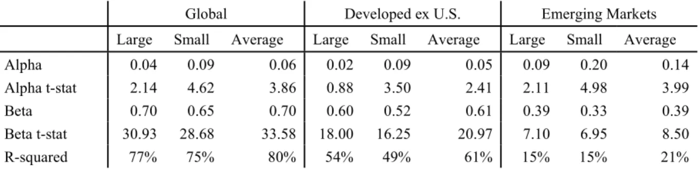
portfolio in the United States in Table 5. All regressions are against the equally weighted factor

portfolio in corresponding size bucket in the US. For example, the equally weighted factor

portfolio in DevxUS large is regressed against the equally weighted factor portfolio in US large.

The only region / size group that fails to earn a statistically significantly positive alpha on

the corresponding US portfolio is DevxUS large, which earns a 2 bp monthly alpha (t-stat: 0.88).

The equally weighted portfolio of factor returns in global large earns a 4 bp monthly alpha (t-stat:

2.14) and EM large a 9 bp monthly alpha (t-stat: 2.11) on the corresponding US large portfolio.

The portfolio in global small earn a 9 bp monthly alpha (t-stat: 4.62) against the US small portfolio.

The DevxUS small portfolio earns a 9 bp monthly alpha (t-stat: 3.50) against the US small

portfolio. The equally weighted portfolio of factor returns in EM small earns 20 bp alpha (t-stat:

4.98) against that of US small. The R-squared of the equally weighted portfolio of factor returns

in a given region regressed against the same portfolio in the US is lower in EM than in DevxUS—

21% in the average portfolio for EM and 61% for DevxUS. Global factors have a high correlation

with US factors because the US makes up a large portion of global market capitalization.

1.2.9 Post-Sample Returns

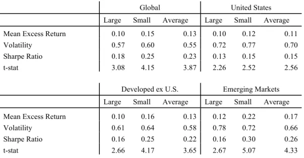
Another potential objection to these results is that they are not post-sample. Table 6 shows

the post-sample equally weighted portfolio results. Post-sample is defined by the first January after

the original paper’s sample period. Sample periods are defined as in McLean and Pontiff (2016).

Similar to Jacobs and Müller (2019), all region / size buckets are significant, though most

buckets have lower significance than in the full sample shown in Table 4.

1.2.10 Covariances vs. Characteristics

Instead of sorting on characteristics, I sort on factor loading in each region in Table 7. For

each stock, I calculate the full period factor loading against the market and one of the 86 factors in

a bivariate regression. I use the average of the large and small factor as the regressor regardless of

whether a large, small, or average factor is tested. I use a full period regression, because I am

testing an asset pricing claim as opposed to a predictive claim. The look-ahead bias in a full period

regression is not relevant since my goal is to test whether the loading on a factor delivers a

particular return as opposed to whether a trader in a given time with the information at hand could

earn excess returns by estimating factor loadings.

When using covariances, far fewer factors are significant. Among global large, three

factors, earnings surprise, profitability, and ROE are significant at a 0.05 level. Among global

small factors and global average factors, earnings surprise, 52-week high, profitability, and ROE

are significantly positive while dividend initiation is significantly negative.

In the US, earnings surprise is significantly positive in the large, small, and average

portfolios. Profitability is positively significant among small stocks. Leverage is negatively

significant in both the small and average portfolios. In DevxUS, earnings surprise, 52-week high,

profitability, and lagged momentum are significant in all size demarcations. Change in profit

margin, profit margin, and ROE are significantly positive in the large and average portfolios.

Earnings consistency is negatively significant in all size demarcations. Percent total accrual is

negatively significant in the large and average portfolios while leverage and size negatively

significant in the small and average portfolios. Momentum-reversal is significantly negative in the

average portfolio.

In EM, dividends are significant at a 0.05 level among small stocks, 52-week high is

significant in the average portfolio, lagged momentum is significantly positive in the large and

average portfolios, momentum is significant in all size categories, and earnings-to-price is

significant among small stocks. Leverage is negatively significant among large stocks.

Table 8 shows that an equally weighted portfolio of factors built from covariances delivers

significantly positive returns in EM small and average but nowhere else. Furthermore, these returns

are subsumed by an equally weighted portfolio of characteristic factors. Table 9 Panel A shows

that in all region / size buckets, except emerging markets large and small a portfolio built from

covariance factors earns a significantly negative alpha, while Table 9 Panel B shows that a

portfolio of characteristic factors earns an alpha on a portfolio of covariance factors in every region

/ size bucket. In other words, factors are driven by characteristics, not covariances.

The results in Table 8 are largely unchanged when using other periods of time to generate

covariance estimates such as trailing 5 year or a 10-year period that includes the trailing and future

5-year period.

1.2.11 Long vs. Short Returns

Numerous papers find that factor returns are driven more by the short side of the portfolio

than the long side. In particular, the return of the capitalization-weighted market portfolio minus

the short portfolio’s return is greater than the long portfolio’s return minus the

capitalization-weighted market portfolio. Table 10 shows the percentage of return that comes from the long side

of the portfolio as a percentage of the total factor return. The number is subject to outliers since

the factor return may be close to 0. However, the median value is above 50% in each region / size

bucket suggesting that most of the return comes from the long and not the short portfolio. In US

Large, the median factor has 50% of the excess return originating from the long and 50% from the

short. In EM Large, the median factor has 63% of the excess return originating from the long and

37% originating from the short. If limits to arbitrage are preventing these factor returns from being

earned, those limits cannot be mere shorting constraints, since the long side of the portfolio

contributes half or more of the excess return.

1.2.11 Factor Volatilities

Table 11 shows the factor volatilities. The long-only market portfolios show a pattern of

increasing volatility from US to DevxUS to EM during this period with a 4.2% monthly volatility

in the US, 4.5% in DevxUS, and 6.4% in EM. While EM factors are the most volatile, DevxUS

factors are less volatile than the US ones. Among the average of large and small factors, 78% are

less volatile in DevxUS than in the US and 23% are less volatile in EM than in the US. The average

of the monthly factor volatilities in the US is 2.80%, in DevxUS 2.29%, and in EM 3.31%.

Table 4 shows that the volatility of the equally weighted factor portfolios is highest in the

US at 0.73%. The equally weighted factor volatility in DevxUS is 0.57% and in EM is 0.63%. In

other words, the correlation among the factors in EM is lower than the correlation among factors

in the US, such that factor diversification benefits in EM are higher. This phenomenon is

manifested again in the principal component analysis performed later in Chapter 2.

1.3 Determining Which Factors Deliver Excess Return

While I show that an equally weighted portfolio of factors deliver returns, I do not indicate

which factors have higher premium. I show here that this question cannot be answered using

historical average return or Sharpe Ratio. In particular, a portfolio that buys the top 30% of factors

with the highest historical mean return and shorts the bottom 30% of factors with the lowest

historical mean return performs does not deliver positive returns generally.

Table 12 shows that in global large and the average of global large and global small, this

strategy of choosing factors that have historically performed well and selling factors which have

historically performed poorly delivers negative insignificant returns. In the United States, such a

strategy produces negative returns in all size categories, significantly so in large stocks. Developed

ex US shows significantly positive returns in small but insignificant returns in large and average.

In Emerging Markets, returns are insignificant in large and average and significantly positive in

small. In short, betting on the factors that delivered the highest historical return does not pay off.

Similarly, inconsistent results hold if we use historical Sharpe Ratio instead of historical

mean return, though in this case, global small, DevxUS small, and EM small all show significantly

positive returns to choosing the best performing factors and shorting the worst performing ones.

The broad conclusion is that future factor return cannot be predicted using inception-to-date mean

return. This isn’t to say that factor returns are unpredictable, just that one cannot determine which

factors will deliver excess returns using historical mean return or Sharpe Ratio, the latter of which

is equivalent to comparing t-stats for factors with equal numbers of observations.

This claim is seemingly inconsistent with the notion that these factors deliver excess

returns, since I claim factors deliver excess return because of their historical excess return and yet

their historical excess return is not an indication of future excess return at any given time. Instead,

what may be occurring is that these factors all have roughly the same positive expected return and

any difference in trailing return is more likely to reflect noise than any particular signal.

1.4 Indicators of market efficiency

I examine aspects of US, DevxUS, and EM markets that might indicate either limits to

arbitrage or lower attention. While such illustrative data is insufficient evidence to make firm

claims, they do support the notion that less attention is paid to emerging markets and that there are

likely greater limits to arbitrage at least as evidenced by lower trading volume in emerging markets.

Using market capitalization-weighted institutional ownership of the top 4000 stocks by

float-adjusted market capitalization from Bloomberg

, the US has averaged 81% institutional

ownership between April 2010 and November 2018, DevxUS 49%, and EM 49%. Globally,

institutional ownership has averaged 65%. Note that institutional ownership includes state-owned

enterprises, possibly explaining the fact that EM and DevxUS have similar institutional ownership.

Globally, among these stocks, institutional ownership increased from 57% to 72% between

April 2010 and November 2018. In the US, it remained roughly the same dropping from 85% to

84%. It increased from 45% to 56% in DevxUS and from 37% to 55% in EM.

Monthly trading volume summed across all stocks in 1996 averaged $559 billion in the

US, $315 billion in DevxUS, and $84 billion in EM excluding Brazil

. By 2018, trading volume

averaged $4,752 billion in the US, $1,530 billion in DevxUS, and $780 billion in EM excluding

Brazil. Volume may be a proxy for attention and limits to arbitrage.

I/B/E/S coverage may be a proxy for attention. However, they cover 22,000 active

companies but Worldscope shows 35,201 active companies in fiscal year 2017 among emerging

and developed markets. In the US, IBES coverage starts at 36% in 1995 and increases to 48% by

2018. In DevxUS, IBES coverage starts at 25% in 1995 and drops to 22% by 2018. In EM, IBES

1 _{The number 4000 was chosen due to Bloomberg download limits. While top 4000 was used as a cutoff for}

downloading, as long as a stock was once in the top 4000, it is subsequently used for analysis.

coverage was 21% in 1995 and drops to 16% by 2018. These drops in percentage coverage are due

to new listings that aren’t covered by I/B/E/S or new exchanges being added to the database at

lower coverage, not absolute drops in number of stocks covered.

1.5 Are markets becoming more efficient?

Given the results of McLean and Pontiff (2016), it may be the case that markets are

becoming more efficient over time. I test this hypothesis by regressing equally weighted factor

portfolios and long-short portfolios built from expected returns against time:

𝑅 = 𝛽 + 𝛽

𝐷𝑎𝑡𝑒 + 𝜖

𝑅

is the factor excess return in time

𝑡

and

𝐷𝑎𝑡𝑒

is the date at time

𝑡

represented in days

since January 1, 1900. The dates are divided by one million for scaling. A coefficient of 2

corresponds to a factor excess return decay of 7.3 bps per year.

For

𝑅

, I use each of the following:

1)

an equally weighted portfolio of factors

2)

long-horizon mispricing, a long-short portfolio built from expected returns using

inception-to-date average coefficients of a regression predicting return using anomaly

characteristics

3)

short-horizon mispricing, a long-short portfolio built from expected returns using

the most recent coefficients of a regression predicting return using anomaly characteristics

Table 13 reports the results of these regressions. All coefficients regardless of size, region,

or method of construction are negative, except for the DevxUS small long-short portfolio created

out of inception-to-date average coefficients.

For an equally weighted portfolio of factors, none of the coefficients are significant at even

a 0.10 level though all coefficients are negative. A long-short portfolio of expected returns using

inception-to-date coefficients shows 0.05 significance in DevxUS large and 0.10 significance in

global large and EM large. Using the most recent coefficients,

𝛽

is significant at a 0.01 level

for global small and average and DevxUS large, small, and average.

𝛽

for US small and EM

small and average is significant at a 0.05 level.

𝛽

for global large and EM large is significant

at a 0.10 level.

The decay appears to be stronger when using the most recent coefficients as if the market

has become savvy to the short-term mispricing but not the long-term structural mispricing,

although the evidence remains too weak to make such sweeping generalizations. However, there

is some weak evidence that anomaly returns are decaying over time.

1.6 Transaction Costs

Due to lack of bid-ask spreads for all stocks, I am unable to measure transaction costs

reliably. However, Table 14 shows monthly one-way turnover, which should ceteris paribus be

linearly related to transaction cost. Factors seem to break cleanly into low turnover and high

turnover factors. For example, among global stocks, slow-moving characteristics like 5-year share

issuance, beta, organizational capital, or Herfindahl (industry diversification) generate monthly

one-way turnovers of 5%, 6%, 3%, and 4%, respectively. Fast-moving characteristics like

short-term reversal, down forecast, up forecast, and coskewness generate monthly one-way turnovers of

147%, 110%, 111%, and 144%, respectively. Assuming a 100 bps transaction cost per 100%

one-way turnover, these high turnover factors would universally generate a negative return.

1.5 Conclusion

The results for factor returns globally suggest that factors are not only robust outside of the

United States but are stronger outside the United States and stronger in markets broadly thought

to be less efficient like small capitalization stocks and emerging market stocks. This suggests that

the lower factor returns post-discovery found by McLean and Pontiff (2016) are likely due to

arbitrage as opposed to data mining since the factors deliver excess returns globally

post-discovery.

Moreover, in all regions, even within the US, an equally weighted portfolio of factors earns

a highly significant alpha on every model currently used to explain anomalies. An equally

weighted portfolio of factors in DevxUS and EM earned a significant alpha on such a portfolio in

the US, suggesting the international factor returns arise from an orthogonal source.

I find that factors are driven by characteristics, not covariances. Consequently, factors built

from expected returns based on characteristics subsume simple equally weighted portfolios and

perform best when explaining factor returns.

Taken together, these results demonstrate that factors deliver excess returns globally, that

there are significant components of factor returns outside the United States that are orthogonal to

factor returns in the United States, and that factor returns as a whole cannot be explained by a

handful of factors. The “factor zoo” bemoaned by Cochrane (2011) is even more multitudinous

than previously thought.

1.7 References

Arkes, Hal R., David Hirshleifer, Danling Jiang, and Sonya Lim. "Reference point adaptation:

Tests in the domain of security trading."

Organizational Behavior and Human Decision

Processes

105, no. 1 (2008): 67-81.

Ben-Rephael, Azi, Ohad Kadan, and Avi Wohl. "The diminishing liquidity premium."

Journal of

Financial and Quantitative Analysis

50.1-2 (2015): 197-229.

Brennan, Michael J., and Avanidhar Subrahmanyam. "Market microstructure and asset pricing:

On the compensation for illiquidity in stock returns."

Journal of Financial Economics

41.3 (1996):

441-464.

Carhart, Mark M. "On persistence in mutual fund performance."

The Journal of Finance

52.1

(1997): 57-82.

Cochrane, John H. "Presidential address: Discount rates."

The Journal of Finance

66.4 (2011):

1047-1108.

Daniel, Kent, David Hirshleifer, and Lin Sun. “Short and long horizon behavioral factors.”

Review

of Financial Studies

. Forthcoming.

Fama, Eugene F., and Kenneth R. French. "The cross‐section of expected stock returns."

The

Journal of Finance

47.2 (1992): 427-465.

Fama, Eugene F., and Kenneth R. French. "Incremental variables and the investment opportunity

set."

Journal of Financial Economics

117.3 (2015): 470-488.

Harvey, Campbell R., Yan Liu, and Heqing Zhu. "… and the cross-section of expected

returns."

The Review of Financial Studies

29.1 (2016): 5-68.

Hirshleifer, David, and Siew Hong Teoh. "Limited attention, information disclosure, and financial

reporting."

Journal of Accounting and Economics

36.1-3 (2003): 337-386.

Hou, Kewei, Chen Xue, and Lu Zhang. “Replicating anomalies.” No. w23394. National Bureau of

Economic Research, 2017.

Hsee, Christopher K., and Elke U. Weber. "Cross‐national differences in risk preference and lay

predictions."

Journal of Behavioral Decision Making

12.2 (1999): 165-179.

Hsu, Jason C. and Vivek Viswanathan. “Illiquidity and Factor Returns: Exploring the Intersection

Between Illiquidity, Small Cap and Popular Factors.”

Journal of Investment Management.

Vol.

16, No. 4. (2018).

Lev, Baruch, and Doron Nissim. "Taxable income, future earnings, and equity values."

The

Accounting Review

79.4 (2004): 1039-1074.

Linnainmaa, Juhani T., and Michael Roberts. "The History of the Cross-Section of Stock Returns.”

Review of Financial Studies

. (2016).

Lintner, John. "Security prices, risk, and maximal gains from diversification."

The Journal of

Finance

20.4 (1965): 587-615.

Liu, Ruomeng. “Asset Pricing Anomalies and the Low-risk Puzzle.”

American Finance

Association

Annual Meeting

. (January 2019).

Lou, Xiaoxia, and Tao Shu. "Price impact or trading volume: Why is the Amihud (2002) illiquidity

measure priced."

Available at SSRN

2291942 (2014).

McLean, R. David, and Jeffrey Pontiff. "Does academic research destroy stock return

predictability?."

The Journal of Finance

71.1 (2016): 5-32.

Merton, Robert C. "On the pricing of corporate debt: The risk structure of interest rates."

The

Journal of Finance

29.2 (1974): 449-470.

Novy-Marx, Robert. "The other side of value: The gross profitability premium."

Journal of

Financial Economics

108.1 (2013): 1-28.

Novy-Marx, Robert. "Testing strategies based on multiple signals."

NBER Working Paper No.

21329.

(2016).

Sharpe, William F. "Capital asset prices: A theory of market equilibrium under conditions of

risk."

The Journal of Finance

19.3 (1964): 425-442.

Shleifer, Andrei, and Robert W. Vishny. "The limits of arbitrage."

The Journal of Finance

52.1

(1997): 35-55.

Spiegel, Matthew, and Xiaotong Wang. "Cross-sectional variation in stock returns: Liquidity and

idiosyncratic risk." (2005).

Weber, Elke U., and Christopher Hsee. "Cross-cultural differences in risk perception, but

cross-cultural similarities in attitudes towards perceived risk."

Management science

44, no. 9 (1998):

1205-1217.

CHAPTER 2: HIGH-DIMENSION FACTOR RETURNS

While attempts have been made to collapse the factor space in the United States to a handful

of factors, I find that these models fail to explain factor returns both within the United States and

within Developed ex U.S. (DevxUS) and Emerging Markets (EM). Many such papers attempt to

only explain significant factors, but models that explain returns can give significant alphas to

insignificant anomalies. CAPM is the biggest such culprit. Most factors have a negative CAPM

beta, so controlling for market excess returns immediately generates numerous significant alphas.

It’s generally the case that models aiming to control for factor returns tend to increase rather than

decrease the number of significant factors.

Cochrane (2011) worries about the proliferation of factors which he termed a “factor zoo.”

The rational models of human behavior cannot justify the existence of so many factors. The

literature broadly takes two approaches to tackling this problem: collapsing the factor space into

far fewer factors or showing that the factors never existed and are the mere result of data mining.

McLean and Pontiff (2016), Harvey, Liu, and Zhu (2016), and Linnainmaa and Roberts (2016)

take the latter approach. McLean and Pontiff (2016) show that factor t-stats halved post-sample in

the United States but wearere agnostic as to whether this came from inadvertent and collective

data snooping or from arbitrage post-publication. Harvey, Liu, and Zhu (2016) argue that t-stat

thresholds should be much higher given the number of hypotheses being tested, suggesting that

most factors that have been found do not meet the new t-stat threshold and thus likely do not earn

a premium. Linnainmaa and Roberts (2016) look at pre-sample factor returns and find that many

factors were insignificant pre-sample again suggesting data snooping. However, Jacobs and Müller

(2019) and the first chapter of this thesis show that these factors worked internationally even

out-of-sample suggesting that they cannot be the mere result of data snooping. In addition, I find that

factor premia tend to be more significant in emerging markets and small cap stocks, suggesting

that limits to arbitrage allow the premia to persist in these universes.

If factor premia are not a mere result of data snooping, then the alternative approach to

mitigating the factor zoo is to explain many factors with fewer factors. That is, perhaps the 97

factors of McLean and Pontiff (2016) are really 3, 4, or 5 factors and can be simply explained

away by these fewer factors. Fama and French (1992) explain several other value factors with their

more parsimonious 3-factor model. The Carhart (1997) 4-factor model adds a momentum factor

to explain mutual fund persistence in return. There was a considerable gap in such multi-factor

models meant to collapse the factor space since Carhart (1997) as more papers were published

proliferating the factor space as opposed to attempting to collapse it. The Fama and French (2015)

5-factor model uses market, value, size, operating profitability, and investments to explain factor

returns. Hou, Xue, and Zhang (2017) use market, size, return on assets, and asset growth to explain

returns. Novy-Marx (2013) uses market, size, asset growth, and return on assets. Stambaugh and

Yuan (2014) use market, size, management, and performance, where management and

performance are built from a cluster of factors. Daniel, Hirshleifer, and Sun (2018) use market,

post-earnings announcement drift, and share issuance to explain factor returns.

I show that these models do not explain factor returns in all regions. Moreover, they appear

to generate significant alphas among factors that do not have significant returns in their own right.

This is a key finding, since several of the above papers restricted their analysis to only factors that

earn significant returns in their own right. Coming to a similar vein but using a different approach,

Kozak, Nagel, and Santosh (2018) find that factor returns cannot be explained with a

characteristics-sparse SDF in the U.S. However, they do find that a few principal components of

factor returns can explain factor returns well.

If the multitude of factors cannot be explained by data snooping nor can they be collapsed

by a handful of factors, then factors are indeed multitudinous. An alternative theory is necessary

to explain such behavior. It is unlikely the case that investors have a precise and multitudinous set

of risks that they are price these 97 factors. However, I do not attempt to posit a theory as to how

there can be so many anomalies in the market.

2.1 Data

As in Chapter 1, I use Worldscope data for financial data and Datastream for market data.

I also employ the same data cleaning procedures including only including all but tiny stocks as

defined by stocks with 20

percentile NYSE market capitalization and above. Factor returns are

similarly calculated as top 30% minus bottom 30% on a given characteristic.

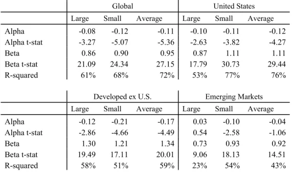
2.2 The Capital Asset Pricing Model (CAPM)

I devote a section specific to the Capital Asset Pricing Model (CAPM), because numerous

factors that do not have significant returns in their own right have significant CAPM alphas, and

this fact demands an explanation. Consistent with Liu (2019), Table 15 shows that many factors

have predictable and persistent negative betas. For example, highly profitable firms and firms near

their 52-week high have lower betas than less profitable firms and firms far from their 52-week

high. Consequently, the CAPM alphas are higher than the monthly returns of those factors.

Many of the factors that have been discovered are quality factors. Insofar as these good

features push a firm farther away from default, then by Merton (1974), these firms should have

lower volatility and beta

ceteris paribus.

In Table 15, I show that most factors have a negative beta. Speaking just among average

factors, 73% (z-score of 4.27 for difference from 50%) have negative beta among global stocks,

66% score: 2.97) in the United States, 78% score: 5.19) in Developed ex U.S., and 60%

(z-score: 1.85) in Emerging Markets. Because market returns are on average positive, this results in

more factors having significantly positive alphas than significantly positive returns. Even if a

factor’s beta is positive and the factor’s return is insignificant, its CAPM alpha can be significant

since the market beta may explain sufficient variance of the factor to make up for the lower mean

return.

While 18 factors are significant in their own right globally at a 0.05 level, 29 factors have

significant CAPM alphas. In the US, there are 20 significant CAPM alphas compared to only 4

significant factors, in DevxUS, 26 significant CAPM alphas to 12 significant factors, and in EM,

26 significant CAPM alphas to 23 significant factors. Interestingly, though more factors are

significant in EM than any other region, EM does not have more significant CAPM alphas than

other regions. Indeed, this is true of all model alphas, not just CAPM. This suggests that the market

is accounting for more of the variation in the factor returns in the US than in DevxUS than in EM.

However, the introduction of CAPM makes factor returns that much more puzzling. There are

more rather than fewer factors to explain.

2.3 Collapsing the Factor Space

I utilize the methodologies of papers that have attempted to explain factor returns using a

handful of factors. Globally, these results do not hold, but more particularly, factors that are

insignificant can earn significant alpha once controls are added. Hou, Xue, and Zhang (2017)

measure alpha of significant factors against their model but do not look at the alpha insignificant

factors.

Tables 16, 17, 18, and 19 show the global, US, DevxUS, and EM alphas, respectively, of

the 86 factors using various models. The first model we use is CAPM (Sharpe (1964), Lintner

(1965)) which regresses the excess return of the factors on the excess return of the value-weighted

market. In this case, the market is the value-weighted returns in a given region. Because all returns

are stated in USD, I use the USD risk-free rate from the French Data Library. Table 20 shows the

summary data on alpha significance using various models.

2.3.1 Fama French 3-Factor Model (FF3)

The 3-Factor model of Fama and French (1992) includes value in the form of

book-to-market and size as measured by negatively sorted book-to-market capitalization. Surprisingly, there are

more significant FF-3 alphas than CAPM alphas, even in the US.

Globally, there’s no obvious pattern for which factors have significant FF3 alphas but not

CAPM alphas. Post earnings drift, revenue surprises, age-momentum, and operating leverage have

positively significant FF3 alpha but insignificant CAPM alpha.

Overall, there are 38 significant alphas globally at a 0.05 level, 29 in the US, 29 in DevxUS,

and 29 in EM.

2.3.2 Carhart 4-Factor Model

The Carhart (1997) 4-Factor Model adds momentum as defined by past 12-month return

excluding the most recent month. Note that this momentum is different from the momentum

measure used by McLean and Pontiff (2016) and originally Jegadeesh and Titman (1993), who

use the past 6-month return. Market anomalies such as 52-week high, age-momentum,

coskewness, industry momentum, lagged momentum, price, and volume trend are explained by

the addition of momentum.

Carhart performs better than either the CAPM or the FF3 model with 29 significant

anomalies globally, 24 in the US, 20 in DevxUS, and 23 in EM.

2.3.3 Fama French 5-Factor Model (FF5)

The Fama and French (2015) 5-Factor model performs better than FF3 and CAPM but not

the Carhart model. FF5 explains some valuation anomalies like cash flow / MV, dividend yield,

and earnings-to-price, but causes the leverage component of B/P, organizational capital, and

R&D/MV to gain significant alphas that were not significant in FF3 or CAPM. Ironically, despite

having an investment factor in the form of asset growth, the investment factor from Titman, Wei,

and Xie (2004) manages a significant FF5 alpha globally. The Titman, Wei, and Xie (2004)

investment factor is measured by capital expenditures scaled by revenue divided by the average of

the prior 3 years capital expenditures scaled by revenue.

Overall, the FF5 model has 32 significant alphas globally at a 0.05 level, 17 in the United

States, 25 in DevxUS, and 14 in EM.

2.3.4 Novy-Marx 5-Factor Model (NM)

The Novy-Marx (2013) 5-Factor model adds gross profitability to the Carhart 4-Factor

model. It explains seven additional anomalies over the Carhart 4-Factor model but also introduces

significant alphas to eight anomalies which had insignificant Carhart 4 alphas. Factors that have

significant Carhart 4 alphas but are explained by NM include post earnings drift, repurchases,

accruals, asset turnover, forecast dispersion, percent operating accrual, and Z-Score. The nine

anomalies explained by Carhart but not NM are age-momentum, Amihud’s measure, volume,

volume variance, volume / MV, dividends, change in capital expenditures versus the industry

average, and dividend yield.

The NM model has 30 significant alphas in global, 19 in the US, 17 in DevxUS, and 22 in

EM.

2.3.5 Hou, Xue, and Zhang 4-Factor Model (HXZ)

The Hou, Xue, and Zhang (2017) q-factor model includes the market, size, return on assets

(ROA), and investments measured as asset growth. The ROE and investment anomalies are built

using a 3 x 3 x 2 intersection with each other and size broken into large and small. Globally, this

model explains less successfully than CAPM, leaving 34 positively significant anomalies to

CAPM’s 33, but it manages to find 6 negatively significant anomalies versus 2 for CAPM.

Negatively significant factors are theoretically as troublesome as positively significant

ones if we believed them to continue to be negatively significant. Conceptually, it is still an

anomaly—one just needs to flip the implementation. However, without a theoretical justification

for why the factor should deliver a negative alpha after controlling for these specific factors, there

is little sense in flipping the sign. The negatively significant factors under HXZ globally are

dividends (whether the stock paid dividends over the prior 12 months), growth in long-term NOA,

sustainable growth, bid-ask spread, price, seasonality, and volume. Asset growth shows a return

negatively significant at a 0.10 level but is also one of the factors in HXZ. The HXZ

implementation is created by creating a 2 x 3 x 3 intersection with size, asset growth, and return

on equity. The negative alpha suggests that such an implementation subsumes the simple asset

growth implementation with a 2 x 3 intersection with size and asset growth. Bid-ask spread is

already negatively significant under the CAPM. None of the others have any obvious reason to

deliver significantly negative alpha after controlling for the market, size, ROA, and investments.

HXZ leaves 34 factors significantly positive globally, 21 in the US, 9 in DevxUS, and 17

in EM. HXZ is the best at explaining DevxUS anomalies.

2.3.6 Stambaugh and Yuan 4-Factor Model (SY4)

Stambaugh and Yuan (2016) clusters a set of factors and used averages of factor returns

within those two clusters to create a management and performance factor. They use market, size,

management and performance to explain factor returns. Similar to HXZ, SY4 increases the number

of significant alphas globally versus CAPM with 34 significant factors rather than CAPM’s 33.

SY4 suffers most in valuation anomalies, with analyst value, book-to-market, cash flow / MV,

dividend yield, earnings-to-price, enterprise component of B/P, enterprise multiple, and sales /

price all being positively significant while leverage component of B/P and R&D / MV are

negatively significant.

Overall, SY4 leaves 34 factors significantly positive globally, 31 in the US, 24 in DevxUS,

and 27 in EM.

2.3.7 Daniel, Hirshleifer, and Sun 3-Factor Model (DHS)

Daniel, Hirshleifer, and Sun (2018) use the market, post-earnings announcement drift,

which captures short horizon mispricing, and the average of one-year and five-year issuance,

which captures long horizon mispricing. The DHS model is most successful at explaining factors

in the US relative to other models discussed thus far. Globally, among anomalies with significant

CAPM alphas, DHS explains the repurchase anomaly, beta, idiosyncratic risk, max (also called

the lottery effect), volume variance, dividend yield, sales / price, asset turnover, and forecast

dispersion.

I maintain the signal in post-earnings drift until the subsequent announcement date due to

the low I/B/E/S emerging market coverage and the need to calculate a signal in every month

globally. I/B/E/S coverage is not as comprehensive globally as it