Glider-based O₂ and CO₂ observations in the Labrador Sea

(1)

Glider-Based O

2

and CO

2

Observations in the

Labrador Sea

by

©Nicolai von Oppeln-Bronikowski

A thesis submitted to the School of Graduate Studies in partial fulfilment of the requirements for the degree of

Master of Science

Department of Physics and Physical Oceanography Memorial University of Newfoundland

May 2019

(2)

Abstract

Ocean gliders can provide high-resolution gas observations necessary to interpret the space and time scales of highly dynamic processes such as gas uptake or outgassing in the ocean surface layer. There is a critical need to make high-resolution in situ gas measurements in the ocean for the biogeochemical community (Johnson et al., 2009). Small optical sensor, called optodes, have been used on gliders to measure dissolved oxygen in the oceans and recently optodes were modified to measure pCO2

(Atamanchuk et al., 2014). The CO2 optode is in an early prototype stage and

has not undergone rigorous testing on a glider. Here we describe our approach to reference glider based O2 and pCO2 measurements to data from a vertical profiler

mooring – the SeaCycler to validate the glider data. The SeaCycler carried a Pro-Oceanus Ltd., CO2-Pro CV as part of its instrument float, an extensively tested

gas analyzer, based on non-dispersive infrared refraction (NDIR), which has shown stable performance during lengthy observations (Jiang et al., 2014). We compare the glider data against the SeaCycler’s O2 and CO2 measurements to compute an

isopycnal-matched in-situ optode correction. We conducted further glider tests of the sensor on the Newfoundland Shelf in 2018 and further characterized the response time in profiling applications. In this thesis, we show data from both deployments to characterize the sensor performance. We discuss the spatial and temporal structure in the Labrador Sea glider data and use frequency and correlation length scale analysis to infer the presence of short internal wave energies near the buoyancy frequency range. From the results of the glider missions, we present ideas to improve future glider missions into the Labrador Sea and glider based CO2 measurements.

(3)

Acknowledgements

This work builds on the contributions of many people. I like to express my sincere gratitude to my supervisor, Brad deYoung, who guided me through oceanography, opened doors when they seemed difficult to open and enabled a wide range of ex-posure to disciplines, people and learning opportunities. Also for saying yes to my ideas more often than anyone I have met before. Dariia Atamanchuk and Chris L’Esperance at Dalhousie University for their help calibrating O2 and CO2 sensors

used in the deployments. Dr Mingxi Zhou at the University of Rhode Island, Robin Matthews at the Universit´e Paris-Saclay and Mark Downey at Memorial University for their help with collecting data and glider deployments. Also special thanks to Len Zedel, Johannes Karstensen and Heather Reader for fruitful discussions. This work was funded through the National Science and Engineering Research Council Canada (NSERC) funded Climate Change and Atmospheric Research Network (CCAR). Last and not least I want to thank my loving girlfriend Julia. Thank you for your patience and for being always there for me.

(4)

List of Figures

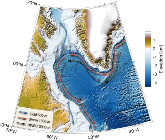
2.1 Map of Labrador Sea and general circulation pattern. . . 9

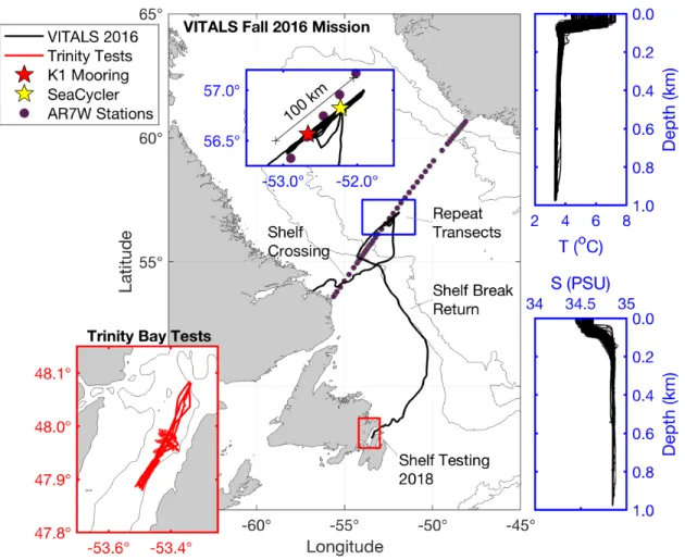
3.1 Map of data collection sites. . . 37

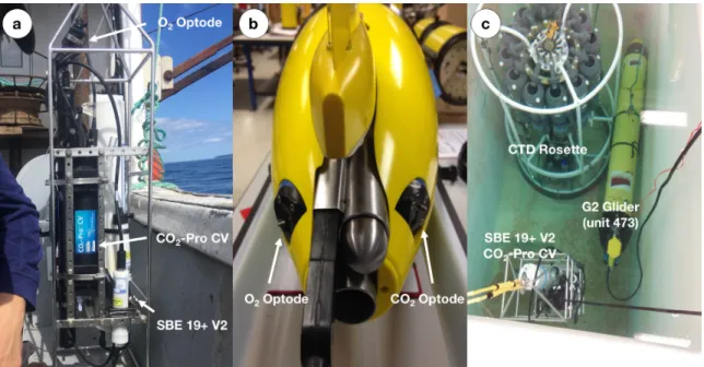
3.2 Instruments and calibration setup for Trinity Bay. . . 40

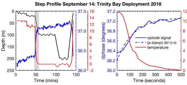
3.3 Example of a step profile used to quantify response time characteristics. 47 4.1 CO2 response time fits and bias. . . 52

4.2 Schematic drawing of the CO2 optode sensing foil. . . 53

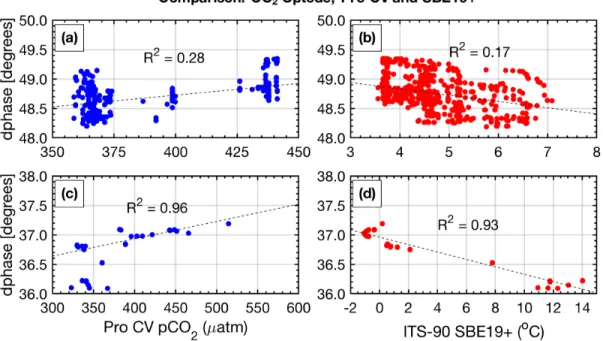
4.3 CO2 optode data comparison between missions and instruments. . . . 56

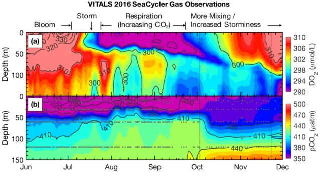
4.4 Glider-SeaCycler O2 and pCO2 isopycnal-matched residual comparison. 59 4.5 SeaCycler O2 and pCO2 time series. . . 60

4.6 Glider monthly averaged spatial section of O2 and pCO2. . . 61

4.7 Glider Hovm¨uller diagram for surface O2 data. . . 63

4.8 Glider Hovm¨uller diagram for surface pCO2 data. . . 63

5.1 Mixed layer depth and surface temperature evolution. . . 66

5.2 Strong mixing event captured by the glider. . . 67

5.3 Convective resistance and potential density record. . . 69

(8)

5.5 Autocorrelation functions for T, S and O₂ in space and time lags. . . 74 5.6 T–S diagram for surface observations. . . 77 5.7 T–S diagram for intermediate depth observations. . . 78 5.8 Column integrated O₂ content and AOU. . . 79

(9)

Chapter 1 Introduction

1.1 Motivation for this Thesis

The motivation of this work starts with the Ocean Observing Conference of 2009 at which the global biogeochemical community asked the autonomous sampling teams across the world to advance remote sampling of CO₂ parameters in the global ocean environment. CO₂ is a critical parameter in the atmosphere and the ocean, intrin-sically linked to the biological and physical processes that have shaped our planet in the past and will in the future. Since Ocean Obs’09, several projects, improving the understanding of the strength of oceanic CO₂ uptake sinks, such as the Surface Ocean CO₂ Atlas (SOCAT) have been made possible by community efforts to reach standards for mobile in-situ sampling technology. However, there is still a lack of regular high-resolution measurements of oceanic CO₂ system parameters in most of the world’s ocean regions. Intense carbon uptake, associated with regions of energetic atmospheric heat exchange such as the Labrador Sea, has raised alarming questions

(10)

about the future role of these regions during times of global climate change. Depth-resolved carbon measurements are a necessity.

Through combined national and international scientific efforts, a dedicated re-search program was funded through the National Science and Engineering Rere-search Council (NSERC), Climate Change and Atmospheric Research (CCAR) network to observe and study the Labrador Sea: Ventilations, Interactions and Transport Across the Labrador Sea (VITALS) program. This program, which encompassed modelling and observational components worked together across scientific disciplines with on-going Canadian and international research efforts to implement a holistic plan to measure some of the short time scale processes of carbon uptake and lateral exchange in the Labrador Sea. This thesis examines the results of the deployment of a glider and vertical profiler – the SeaCycler, in the Labrador Sea. We present the data and our analysis and discussion around central themed questions:

• How to measure CO₂ using gliders in the open ocean?

• How can multiple autonomous platforms be used to help improve sensor data?

• How to best observe spatial and temporal structure with gliders in the Labrador Sea?

Answering these questions is critical, to improve and shape our current and future plans for carbon observing systems utilizing glider and other platforms, especially as new technology is being developed such as new CO₂ or pH sensors. We also present new observations of fall conditions in the Labrador Sea, a very dynamic ocean frontier.

(11)

1.2 Marine CO

₂

and Carbon Observing Needs

The global ocean system plays a crucial role in absorbing the effects of changes to the Earth’s atmospheric composition due to anthropogenic activities. Roughly one-third of all anthropogenic CO₂ (Cant) released into the atmosphere since the beginning of

the industrial revolution has been taken up by the ocean, a total of 155 ± 31 PgC as of 2010 (Khatiwala et al., 2013). Increased CO₂ levels are directly linked to an increase in free hydrogen ions causing a decrease in pH, at a rate of change that is faster than any time in the past geological record (Zeebe et al., 2016). This decrease in pH, termed ocean acidification (OA), causes detrimental effects on marine habitats by disrupting carbonate mineral saturation states affecting, for example, the growth of corals (Cohen and Holcomb, 2009; Guinotte and Fabry, 2009).

The uptake of CO₂, however, does not happen equally in the ocean, as colder surface waters in northern and southern latitudes have higher CO₂ solubility (Volk and Hoffert, 1985). Key oceanic sites in the world act as global carbon sinks also termed solubility pumps, such as the Labrador Sea (DeGrandpre et al., 2006) and the Weddell Sea (van Heuven et al., 2014). These sites undergo deep vertical mixing in the wintertime bringing atmospheric CO₂ to deep water mass transports such as the Atlantic Meridional Overturning Circulation (AMOC) through which carbon can spread to the rest of the world’s ocean (Broecker, 1991; Fontela et al., 2016). In addition to these physical processes, plankton and bacteria contribute to top layer biological pumping of oxygen and carbon dioxide through uptake and respiration which increases the carbon content in the upper water column before convection takes place (Azetsu-Scott et al., 2010). Linking the global ocean system to the carbon

(12)

uptake in these regions must be studied to assess the rate of OA. There is a critical need for a global ocean carbon measurement system because existing observations are limited in coverage and quality (Borges et al., 2010; Okazaki et al., 2017). Some are calling on recent advances in autonomous sampling strategies, such as ocean gliders (Rudnick, 2016), to form a biogeochemical observing network (Johnson et al., 2009).

1.3 The VITALS Program

Advancing autonomous measurements of critical biogeochemical variables such as CO₂, are complicated by technology, data quality and logistical challenges around organizing scientific observing programs. Yet, we cannot delay new observations until a perfect solution is achieved, as time and spatial scales of carbon-ocean dynamics are impacted by anthropogenic climate change. Nor do we believe autonomous in-situ sampling capabilities will be improved without deploying current state-of-the-art technology and accepting a certain element of risks associated with pioneering missions.

A key ocean region connected to the widespread impact of increased anthropogenic carbon emissions into the atmosphere is the Labrador Sea. The confluence of different water mass transports, contrasting freshwater influx and atmospheric forcing, leads to large interannual variations of ocean dynamics on all scales, focused in a com-paratively small ocean region. This makes the Labrador Sea a challenging and vital ocean basin for the physical-biogeochemical sciences (K¨ortzinger et al., 2004; Kieke et al., 2007; Yashayaev and Loder, 2009). The important work and data amassed over decades through direct observations, modelling and reanalysis, have put the Labrador

(13)

Sea in prime focus as a regulator of deep ocean carbon content (Sabine et al., 2004; Sabine and Tanhua, 2010). As part of the VITALS project, we devised an observing strategy to carry out novel in-situ observations to:

• Reach the deep convection region with a glider to carry out sampling with the novel foil-based pCO₂ sensor from Aanderaa with minimal ship resources for launch and recovery

• Use measurements provided by the autonomous SeaCycler profiler carrying the larger payload CO₂-Pro CV instrument for glider in-situ calibration points.

This mission presents one of the first attempts to use a moored sensing platform as an in-situ reference point for experimental sensors deployed on a glider to advance data quality and coherence of novel biogeochemical measurements. This is an im-portant step towards increasing the spatial and temporal coverage of oceanic carbon measurements as technology is playing a catch-up game. We extended this mission in September 2018 on the Newfoundland Shelf, in Trinity Bay, to further test the con-cept, flying the glider near a small fishing boat from which reference casts were taken using the same Pro CV instrument. We utilize these two real ocean deployments to improve sensor characterization and the quality of the collected data.

1.4 Chapter Overview

This thesis is composed of six chapters, with a comprehensive background review, Chapter 2 summarizes the standard oceanographic and geographic role of the Labrador Sea region. This section also reviews theory on CO₂ uptake, storage and exchange

(14)

to present a good basis for the remaining chapters. We also introduce available sens-ing technology for CO₂, and past glider deployments into the Labrador Sea as any remote operations in this harsh environment require significant effort and skill in post-processing the data. Chapter 3, reviews the collected data, the strategy and methods with which we processed data. Chapter 4, discusses the glider sensor data with regard to the earlier raised questions on improving CO2 sensing capability, while

Chapter 5 explains glider oceanographic and other observations in the Labrador Sea not discussed explicitly in Chapter 4. The final section - Chapter 6, summarizes re-sults of this work with an outlook for carbon sampling in this region using gliders and other autonomous platforms.

(15)

Chapter 2 Background

2.1 Labrador Sea

The oceanography of the Labrador Sea is complex and fascinating. The strong sea-sonal character of high latitude oceans is present on all scales with strong gyres fed by the Atlantic and polar glaciers from the Arctic that give rise to strong gradients in temperature, salinity, eddies, jets and turbulent mixing plumes (Clarke and Gascard, 1983). Severe storms, harsh temperatures, sea ice – makes this place a real ocean frontier. Yet, this harsh environment is full of life, and this abundance, in physical and biological terms, has created a unique ecosystem. Being a gateway to the Arc-tic adds another strategic and poliArc-tical layer to the Labrador Sea and its bordering countries. The literature on this region is voluminous, here we briefly review some of the geography and oceanography of the Labrador Sea (Lazier and Wright, 1993; Cuny et al., 2002) with a focus on the winter period deep vertical convective mixing (Lazier, 1973; Clarke and Gascard, 1983; Lilly et al., 1999). We focus our review on

(16)

the importance of this region for global marine CO₂ sequestration and transport as part of ongoing research efforts on carbon uptake by the ocean (Sabine et al., 2004; DeGrandpre et al., 2006). Over the past twenty years, there have been several mas-ters and doctoral theses on this region that have greatly benefitted the content of this Chapter (Frajka-Williams, 2009; Landsch¨utzer, 2014; Wolf, 2017).

2.1.1 Geography

The Labrador Sea is located in a deep, roughly oval-shaped basin (on average about 3500 m deep) in the Northern Hemisphere between the coastlines of Labrador and Greenland to the West and East, separated in the North by a shallower sill (approx-imately 1000 m deep) from Baffin Bay; and meets with the North Atlantic to the South. The Labrador Shelf is shallow (less than 500 m) and much more extensive (over 200 NM) than the shelf on the Greenland side, just 10-20 NM to the shelf break. Sharp topography on the Greenland and Labrador Side constricts Arctic airflow giv-ing rise to the substantial fall and winter Northeasterly winds feared by seafarers.

Proximity to the Arctic results in active biological seasonal cycles where the in-jection of nutrients caused by upwelling from glaciers and ensuing transport from currents cause intense blooms of phytoplankton in the spring (Arrigo et al., 2017). Increasing sea ice decline in the Arctic as part of climate change are extending bloom conditions and second blooms in the fall have been observed (Ardyna et al., 2014). The cold winds and temperatures also lead to significant sea ice presence on the shallow Labrador Shelf side in most of the years, but ice is not as extensive on the Greenland side (Parkinson, 2000). Sea-ice cover extends over the majority of the

(17)

Figure 2.1: Map for the Labrador Sea Region. Arrows indicate the approximate path of the cyclonic gyre circulation, including the Deep Western Boundary Current (DWBC). Colors indicate major topographic features.

Labrador shelf, forming in mid-Winter and usually staying until mid-May to early June before being swept South, although formation is not zonally uniform and there is considerable interannual variability in sea ice cover (Prinsenberg et al., 1997). In pack ice formations, strong ice pressure ridges can form keels up to 20 m deep (Sudom et al., 2011) in some places extending to the seafloor, anchoring drift ice, resisting

(18)

winds and currents. Sea-ice is also an important region for the local population in terms of mobility for fishing, and hunting and travel as many coastal communities are without roads (Bell et al., 2014). Winds cause shear and cracks in the ice that form open water zones or Polynyas, and these tend to repeat in the same location making them essential to local marine life and the people that depend on them (Stirling, 1980; Schledermann, 1980; Durkalec et al., 2015). Greenland’s glaciers inject many icebergs into the Labrador Sea, travelling southwards along the Labrador Coast until meet-ing the warmer North Atlantic near Newfoundland, makmeet-ing this region colloquially known as iceberg alley (Robe et al., 1980). These white bolides are a silent reminder of the Arctics enduring influence on the North Atlantic.

2.1.2 Circulation

The main circulation pattern in the Labrador Sea is cyclonic, consisting of the West-Greenland Current (WGC) on the western part of the basin and Labrador Current (LC) to the east. These shallow and narrow jets flow along the coastal shelf breaks slopes, with mean WGC transports of 3 Sv (1 Sv = 1×106 m3 ·s−1) measured at Cape Farewell (Clarke, 1984) and LC summertime transport of 11 Sv, but seasonal variations of up to 4 Sv noted by Lazier and Wright (1993). The changes in flow strength are influenced by Arctic freshwater flux (Lazier and Wright, 1993). This gyre rotates waters along the Greenland and Labrador coastlines leading to almost saucer-shaped isopycnals in the basin (Lazier, 1973). The WGC introduces warmer-salty water from the Irminger Sea (ISW) and cold-fresh water from the Nordic Seas to the Labrador Sea. This duality results in a layered flow with fresh-cold (θ ≈ −1.8◦C

(19)

and S ≈34.4 PSU) water at the surface and (θ ≈ 4.5◦C and S ≈34.9 PSU) ISW at the bottom of the flow (Cuny et al., 2002). The Labrador Current is fed by Baffin Bay, glacial waters, cold-fresh and nutrient-rich, with (θ ≈ −1.5◦C and S≥34 PSU). ISW has been observed to travel around the basin below this fresh part of the LC preserving the layered structure of the WGC (Cuny et al., 2002). This cold and nutrient-rich water feeds the fertile spawning grounds that makes Newfoundland and the shores of Labrador important fishing grounds for codfish and salmon, both of which have substantially declined in recent decades (Brice-Bennett, 1992; Murray et al., 2007). The deep circulation in this basin is cyclonic consisting of the Deep Western Boundary Current (DWBC) flowing along the 3000 m isobar, carrying North Atlantic Deep Water (NADW) and denser Denmark Strait Overflow Water (DSOW) south. Both currents systems flow into the North Atlantic passing by the Flemish Cap Fischer et al. (2004). Figure 2.1 shows the topography (elevation and bathymetry) of the region, with Labrador (LC) and West Greenland Currents (WGC) divided into fresher (blue) and saltier (red) layers, coinciding with 500 and 1000 m isobaths. Dashed arrows indicate the approximate path of the Deep Western Boundary Current (DWBC) along the 3000 m isobath.

The basin gyre circulation follows the contours of f /h, where f is the Coriolis parameter and h is bathymetry (Cuny et al., 2002). Changes in bottom topography and conservation of potential vorticity lead to frontal instability that gives rise to buoyant anti-cyclonic eddies on the Greenland and Labrador shelf that propagate inward observed from satellites and gliders (H´at´un et al., 2007). A particular type of eddy sheds off Cape Desolation (Greenland). These are called Irminger Rings (Lilly et al., 2003). Another source of eddies is the baroclinic instability observed in the

(20)

central basin influenced by the layered gyre structure. Under the influence of winds or propagation of other activities, the weak stratification gives rise to small scale jets and vortices can mix water vertically to depths over 1000 m and play important roles in restratification of the Labrador Sea after wintertime mixing (Lilly and Rhines, 2002). These interior eddies are believed to regulate heat loss and restratification of the water following wintertime mixed layer erosion (Katsman et al., 2004). Chanut et al. (2008) categorizes these eddies based on the instability source and general region in which they occur.

2.1.3 Convection

The Labrador Sea is one of few ocean regions, where wintertime mixing of the surface layer can reach depths of up to 2000 m (Lazier, 1973; Marshall and Schott, 1999). This deep convection forms a characteristic water lens that occupies a large volume of the Labrador Sea, termed Labrador Sea Water (LSW). The LSW occupies a large volume inside the basin from about 500 to 2000 m in depth and is observed in most of the intermediate depths (1000 to 3000 m) of the North Atlantic and along the Western Boundary past the Equator (Wallace and Lazier, 1988). A Temperature– Salinity (T–S) signature uniquely identifies this water mass from the time that it formed that varies between convection years.

The exact process by which deep convection occurs in the Labrador Sea has been studied for decades and researchers mostly agree on a basic three-phase model adapted from the Mediterranean Sea by Lazier (1973) and Clarke and Gascard (1983). In this model, the process begins with the conditioning of the interior region by the cyclonic

(21)

boundary currents. The horizontal slope of the isopycnal contours draws weakly stratified boundary current water to the interior region. Cold Arctic winds drive surface layer heat loss of over 1000 W/m2 _{(Lilly et al., 1999) that further erode the}

stratification of the surface mixed layer. The second phase starts with storm events or other sources of energy such as eddies, that perturb the delicate vertical balance causing the water column to collapse in the form of turbulent mixing jets or plumes. These plumes quickly mix downward, reaching sometimes up to 2000 m deep (Clarke and Gascard, 1983; Lilly et al., 1999). The resulting mixing exchanges energy in the form of heat and, following a very energetic and short-lived convection period, the surface re-stratifies. This is also referred to as ventilation (van Aken et al., 2011). This intense mixing is made possible by a weak salinity gradient in the Labrador Sea between the surface and the intermediate-depth (200 to 1000 m) water. Finally, spring sea ice melt and warming temperatures restore the density stratification in the water column, forming a several hundred-meter thick surface layer on top of the newly formed LSW, visible in hydrographic sections with its distinct density signature. The final stage of the LSW formation process is the spreading of the water mass along isopycnal slopes of deeper bottom water, feeding the lower limb of the Meridional Overturning Circulation (MOC), pushing this nutrient-rich and oxygenated water mass to greater depths as it travels south along various pathways (Lumpkin and Speer, 2003). Improved knowledge surrounding the LSW formation process is crucial to improving our understanding of the thermohaline circulation model (Broecker, 1991) and the Labrador Sea an important ocean site to understanding the implications of climate change (Kieke et al., 2007). The circulation and transport of LSW is not a significant focus of this background section, but drifter work by Van Sebille et al.

(22)

(2011) focused on DWBC transports have shown latency between LSW formation and travel to 26◦N of approximately 4 years.

Significant inter-annual variability exists in both the strength of convection and volume of LSW production. Pickart et al. (2002) explain this variance through correla-tion with the dominant mode of atmospheric variability called the North Atlantic Os-cillation (NAO). However, in more recent years this explanation has been deemed too simplistic by the general oceanographic community (Chanut et al., 2008). Yashayaev (2007) has shown this variability in LSW formation extends to decadal and multi-decadal cycles, including years with no convection, from over 40 years of hydrographic data. Earlier observational studies in the 1960s (Clarke and Gascard, 1983), describe years with no convection at all, coinciding with a period of low salinity anomalies between 1968 – 1982 (Dickson et al., 1988). This distinct period called the Great Salinity Anomaly of the North-Atlantic is thought to be the result of increased polar freshwater influx advected through the North Atlantic current system and thereby changing convection and LSW formation (Malmberg, 1969; Lazier, 1980). Work by Broecker et al. (1985) and Aagaard and Carmack (1989) pointed towards the danger of increased melt rates in the Arctic and shutdown of convection driven overturning circulation. Most recently Lozier et al. (2019) summarized the work of the Overturn-ing in the Subpolar North Program (OSNAP) – a multi-national effort to directly measure the overturning circulation that forms in the North Atlantic. Based on the OSNAP data, Lozier et al. (2019) challenge the prevailing view of the role of LSW for-mation and MOC strength (Broecker, 1991). Their data (collection started summer 2014) points towards the Irminger and Iceland basins as hot spots for explaining the variability in the MOC strength of the subpolar gyre and a weaker signature of the

(23)

Labrador Sea towards the overturning circulation across the Subpolar North Atlantic, but note the importance of freshwater flux on total transport budgets. The authors of the study, however, acknowledge that more data is needed to capture variability that could exist on longer time scales. The Labrador Sea convection is still a vital heat sink for the world ocean warranting a continued focus on convection strength and variability in LSW formation.

2.1.4 Labrador Sea and the CO

2

Sink

Increasing greenhouse gas concentrations, such as CO2 from burning fossil fuels have

far-reaching influences on our climate. According to the latest report by the In-tergovernmental Panel on Climate Change (IPPC), the increased atmospheric CO2

concentrations have already caused an increase in global temperatures by 1.5◦C. The increasing trend of atmospheric CO2 levels is also being detected in our oceans with

far-reaching consequences to marine life. In fact, we now know that the ocean is re-sponsible for the yearly uptake of about 26% of anthropogenic CO2 emitted into the

atmosphere (Le Qu´er´e et al., 2015). Through this uptake, so far the world’s oceans have had a moderating effect on the progression of global anthropogenic climate change taking up roughly one-third of all anthropogenic carbon emissions since the start of the industrial revolution (Khatiwala et al., 2013). Sabine et al. (2004) com-piled available marine CO2measurements and showed a strong latitudinal increase of

anthropogenic CO2 content in the North Atlantic, with highest concentrations found

in the subpolar regions such as the Labrador Sea. Researchers such as Takahashi et al. (2002) on the other hand compiled atmospheric and marine surface measurements of

(24)

pCO₂ and used the methods from Wanninkhof (1992) to compute atmospheric flux rates for the global ocean as well as looking at seasonal variations due to effects of biology and temperature. His results similarly showed the most considerable flux to occur in subpolar regions such as the Labrador Sea, although his results also showed a substantial seasonal variability from biogenic factors. Watson et al. (2009) also showed that the North-Atlantic is one of the most active sinks of anthropogenic CO2

in the Ocean. Earlier tracer experiments by Wallace and Lazier (1988) similarly pointed to the Labrador Sea convection region as a critical driver in air-sea exchange and uptake of atmospheric gasses.

Theory suggests that atmospheric interaction from storms coupled with high sol-ubility gradients strengthen air-sea fluxes in the North Atlantic, together with deep drawdown through deep wintertime mixing (Clarke and Coote, 1988; DeGrandpre et al., 2006; K¨ortzinger et al., 2008). This has led to notions of the Labrador Sea as a sink for atmospheric carbon. This points to the importance of the Labrador Sea for CO2 uptake and the relevance of programs such as VITALS. Current estimates put

Atlantic Ocean anthropogenic CO2 uptake to −0.45±0.15 PgC·yr−1 (Landsch¨utzer

et al., 2014). However, questions remain as to how much of this contribution is due to the Labrador Sea alone. Much uncertainty remains around how the CO2 uptake

in the Labrador Sea is expected to respond to future global warming and salinity changes due to polar meltwater entrainment (Dickson et al., 2007). This might have severe impacts for global atmospheric CO2 levels further exacerbating greenhouse

ef-fects with implications on marine and terrestrial ecosystems on all scales (Stouffer et al., 2006).

(25)

2.1.5 Wind-Driven Air-Sea CO

₂

Flux Models

The previous section pointed to the Labrador Sea as a global sink for atmospheric CO2. Here we discuss conventional methods to quantify the exchange of CO2between

ocean surface water and the atmosphere and their relevance to estimating CO2uptake

in the Labrador Sea. The relationship between atmospheric CO₂ (xCO₂) and oceanic uptake is usually expressed in the form of bulk flux calculations, were k is the gas transfer velocity (typically mol·s−1) and pCO_2wand pCO_2arefer to the partial pressure of CO₂at the bottom (surface) and top (air) of the sea surface boundary layer across which the flux is to be estimated. This approach is based on a simple model in which mass transport is constrained by turbulence and molecular diffusion (J¨ahne et al., 1987; Landsch¨utzer, 2014). The ocean in such a model is either taking up or outgassing CO₂ and was the basis of the uptake maps produced by Takahashi et al. (2002). This model is somewhat simplistic as it is centred on the surface mixed layer of the ocean. Multi-layer approaches have also been developed, such as Sarmiento (2006), where gas transport is governed by Fick’s first law. For the Labrador Sea wintertime convection, however, where mixed layer depth occasionally reaches to depths over 2000 m, this approach can be used to represent the deep ocean sequestration of CO₂.

d[CO2]

dt =k(pCO2w−pCO2a) (2.1)

In the above formulation, the transfer velocity k is the primary factor that connects air-sea gas exchange to the state of the atmosphere. J¨ahne et al. (1987) was the first to propose a relationship between wind speed (although he called it friction veloc-ity) and Schmidt number (Sc). Wanninkhof (1992) proposed an empirical method

(26)

to compute the Schmidt number for CO₂ for temperatures between 0 to 30◦C and salinities between 0 to 35 ppt. Wanninkhof, using wind tunnel studies, came up with a quadratic relationship of the wind speed at 10 meters (U10) compared with J¨ahne’s

friction velocity. However, different parameterizations of this wind speed coefficient have since been published (Nightingale et al., 2000), and Wanninkhof himself later revised his wind speed relationship to cubic (Wanninkhof and McGillis, 1999).

The above models and parametrizations are only an approximation for the total net flux of CO2 between the atmosphere and the surface ocean. As stated in the

paragraph above, due to the deep mixing in the Labrador Sea in the winter and early spring, surface CO2 concentrations occasionally mix to depths greater than 2000 m.

This makes a 2-layer bulk model a possible approach to estimate total uptake in this particular region. The above models require measurements of the oceanic and atmospheric partial pressure of CO2. The next section will describe the implication

of increased CO2 uptake into the Labrador Sea, highlighting the need for continuous

monitoring of marine carbon parameters. The remainder of the chapter will describe ocean gliders as a measurement platform for the Labrador Sea and introduce various mobile in-situ CO2 sensor technologies with a focus on measurable marine carbon

parameters.

2.2 Implications of Labrador Sea CO

₂

Uptake

During the Labrador Sea deep convection phase, atmospheric CO2 enters the deep

ocean and is distributed globally through deep water mass transports. However, in-creasing CO2concentrations and marine life exist in a delicate balance. The carbonate

(27)

equilibrium reactions (Millero, 2007), show that in presence of seawater, CO₂ under-goes spontaneous dissociation to carbonic acid, releasing free hydrogen ions (Equation 2.2a and 2.2b). These free hydrogen ions (H+_{) are neutralized by carbonate (CO}2–

3 )

ions in water (Equation 2.2c), released from calcium carbonate minerals (Equation 2.2d).

CO₂(g) CO₂(aq) (2.2a) CO2(aq) + H2O H++ HCO3– (2.2b)

HCO₃– H++ CO₃2– (2.2c) Ca2++ CO32– CaCO3(s) (2.2d)

Increased CO2concentrations in an marine environment can completely deplete

avail-able carbonate ions to the point where H+ and HCO3– ions begin to dissolve calcium

carbonate minerals (CaCO3) found in most marine organisms, disrupting ocean life.

The decrease in pH levels from increased H+ concentrations is termed Ocean Acidi-fication (OA). This phenomenon has brought under threat entire ecosystem such as the Great Barrier Reef in Australia (Cohen and Holcomb, 2009). The potential for calcium carbonate mineral to undergo dissolution into carbonate ions due to carbonic acid is defined by its saturation state (Ω) and is controlled by the product of dissolved carbonate mineral ion concentrations and its equilibrium constant (Ksp).

Ω = [Ca

2+

][CO32–]

Ksp

(2.3)

If Ω≥1 then calcium carbonate dissolution does not occur. If it is less, then calcium carbonate mineral will dissolve in seawater, including calcium carbonate from shells found in most of marine life. The most common naturally occurring forms of calcium

(28)

carbonate mineral in seawater are calcite and aragonite and it is common to express calcium carbonate saturation states for aragonite and calcite. The abundance of carbonate ions in a given body of water, with a particular temperature, salinity will lead to depths where saturation drops below equilibrium required to maintain mineral CaCO3. This saturation depth forms a chemical boundary whereby water becomes

to corrosive for marine life to calcify and survive.

Researchers at the Bedford Institute of Oceanography (BIO) are studying how the saturation horizon for calcite and aragonite are affected in the Northwest Atlantic. From ship cruises and bottle samples, in 2010, the estimated Labrador Sea calcite saturation depth reached to 2300 m, coinciding with the LSW formation depth. Arag-onite saturation depth similarly fell within water mass boundaries between LSW and NEADW (Azetsu-Scott et al., 2010). As CO2 concentrations continue to increase in

the atmosphere, these saturation ceilings could change rapidly with deep convection in the Labrador Sea. The formation of a large volume of LSW with high dissolved CO2

concentrations could rapidly deplete available carbonate ions, decreasing carbonate mineral saturation horizons. Such a scenario would threaten the entire Labrador Sea ecosystem. Not to mention the Labrador Sea is home to deep water corals, whose ancient lives may hold untapped clues to the fragile balance of life in the past (Adkins et al., 1998; Sherwood and Edinger, 2009). Due to the links between the Labrador Sea water formation and the global ocean, such rapid changes to the seawater chem-istry in the Labrador Sea would have strong implications for marine life elsewhere. Acidic LSW would eventually make its way to other parts of the ocean, disrupting marine life in those habitats. As climate change continues to affect physical cycles in the ocean and ecosystem health, accurate knowledge of carbonate ion concentrations,

(29)

pH levels and pCO₂ will continue to matter to nations and stakeholders around the world.

2.3 Measurable Marine CO

₂

Parameters

CO₂ in the ocean, despite its importance to crucial climate processes, is still poorly sampled. Long term (monthly sampled) time series (since 1980) only exist in a few places, e.g. the Hawaii Ocean Time Series (HOT) and the Bermuda Atlantic Time Series (BATS) and mostly rely on ship support (Dore et al., 2009; Ducklow et al., 2009). The ocean is still severely undersampled with respect to chemical observations. The cost of ship-based observations and increasing funding challenges to large scale observing programs, has led some researchers to call for an autonomous biogeochemi-cal observing network (Johnson et al., 2009) to increase the resolution of observations. However, this observing component development requires stable measurement tech-niques from in-situ platforms, a challenge that is not yet overcome. Improvements in resolution and frequency of surface CO₂ measurements have been made with the development of stable ship-based in-situ measurement systems installed on vessels of opportunity (VO) such as containerships or tankers with regular routes across ocean basins. These results made possible the creation of a 1◦ global resolution (up to 1/4◦ coastal zones) Surface Ocean CO2 Atlas (SOCAT), initially released in 2011 and

cur-rently distributing the 6th version of this product (Bakker et al., 2016). Any of two of the measurable carbon parameters: pH, Total Alkalinity (TA), the partial pres-sure of CO2 (pCO2) and Total Inorganic Carbon (TIC) are sufficient to calculate all

(30)

used to compute other carbon parameters such as DIC (Dissolved Inorganic Carbon) through equations (Lewis et al., 1998). Of all measured CO₂ parameters, pCO₂ is probably the most prolific measured parameter today due to its relationship between atmospheric concentration and CO₂ flux into the surface ocean through bulk flux calculation methods discussed previously.

Traditional measurements of pH, TIC, TA and pCO2 are typically done through

discrete sampling from shipboard CTD-rosettes equipped with Niskin bottles. Bot-tle samples are taken and analyzed on board the vessel or later on shore using infrared, electrochemical, spectrophotometric (Clayton and Byrne, 1993) and mas-spectrometer type (Yao and Byrne, 1998) methods to analyze gas content and ele-mental composition of CO2 in seawater. A great deal of effort is expended in proper

sample preparation and avoiding contamination from biogenic and atmospheric fac-tors after the sample is taken. Correct salinity and temperature information are also required. On the other hand, in-situ methods are still not very common except for pCO2 and pH (Clarke et al., 2017a). These components have been reliably measured

through infrared (IR) detection in equilibrator type (DeGrandpre et al., 1995) and glass-electrode approaches (Dickson, 1993). There is a strong push in the biogeochem-ical community to increase and expand available in-situ technology to other carbon variables and decrease dependence on ship cruises. Also measuring carbon parame-ters in a discrete sampling way makes it difficult to resolve some of the very localized and short time scale processes by which carbon enters the coastal and open ocean important for getting the physics right in biogeochemical models (Denman and Gar-gett, 1983; Sarmiento and Gruber, 2002). The next sections will discuss the current state of CO2 in-situ sensor technology with a particular focus on mobile platforms

(31)

such as gliders and floats.

2.4 Gliders used for Labrador Sea Observing

Gliders are small cylindrical shaped ocean observing platforms that use changes in buoyancy to float up and down and generate lift by its wings to achieve forward motion. This makes gliders very energy efficient and missions of up to a year are possible (Eriksen et al., 2001). Missions of 4 to 6 month are routine. Upon surfacing, gliders relay information via satellite to the shore servers, offering a close to a real-time look at ocean environments. Typically, gliders are designed for diving to 200 or 1000 m in depth, although new gliders are being tested to go as deep as 6000 m (Osse and Eriksen, 2007). Seen as a visionary solution to achieving higher spatial and temporal ocean resolution to fill gaps left by other observing platforms (Stommel et al., 1989), hundreds of gliders today are used on all continents and ocean regions and collecting valuable high-resolution data for the ocean science community. In conjunction with its sibling instruments, Argo floats of the International Argo program; gliders have become a central part of the Global Ocean Observing Systems (GOOS) (Testor et al., 2010, 2019).

Gathering data through gliders offers several advantages, compared to traditional ship-based surveys, because they are cheaper and easily adaptable to different mis-sions. Autonomous platforms also require less personnel and data can often be ac-cessed in near real time making them ideal for ocean monitoring applications. Called autonomous, though mostly operated by human-pilots through computer commands and scripts, these vehicles are not as self-reliant as their name might suggest. Adaptive

(32)

sampling and path planning work is being done to take away some of the significant efforts on the part of the pilot to keep these vehicles alive during long deployments (Fiorelli et al., 2003; Alvarez and Mourre, 2012). On the downside, they move more slowly (1 km/hr) than ships, meaning time variability is easily aliased as spatial vari-ability (Rudnick, 2016). This makes gliders only moderately suitable for basin-scale observing and most work with gliders has focused on the coastal and intermediate zones, studying shorter spatial scales (Rudnick, 2016). More importantly, glider plat-forms impose a range of restrictions on the type of sensors a glider can carry. Sensors must be small in size to avoid negative impact on hydrodynamic efficiency and must be low weight not to shift the centre of gravity, negatively affecting the buoyancy of the system. The most stringent restriction gliders place on potential sensor probes are restrictions on power consumption that dictate the battery budget and viable length of a mission (Rudnick et al., 2004). Sensors need to be designed explicitly for gliders, and already available sensors that work well with other platforms may not be at all suitable for gliders without substantial modification and testing.

Doing glider work in any remote regions has many challenges, especially in the Labrador Sea. The distance from nearby coastal communities typically requires a ship for launch and recovery or significant battery budget constraints to operate for long periods remotely, constraining the scientific mission. Launching from a ship has certain advantages, as it allows concentrating battery power on collecting relevant sci-entific data, but increases the cost of the mission, environmental footprint and limits deployment to the ship’s availability. Launching from shore brings independence, but requires skill in piloting and can take away months from the mission. Such a launch into the Labrador Sea is a little easier to do from Greenland than Labrador shelf

(33)

side because the shelf break is closer to the coast and gliders can dive to their full depth sooner, making the buoyancy pump more efficient. Launching on the Labrador side would require a glider to dive to 100–200 m for 200 NM, while also confronting the strong boundary currents. As most of the battery draw on a glider comes from the buoyancy pump, increasing dive cycles would result in higher energy loss over a shorter distance.

To date, there have been about a dozen glider missions with sampling focus on the Labrador Sea. Of these deployments, notably Howatt et al. (2018) used a Labrador shelf glider deployment with repeat shelf crossings to quantify heat and salt trans-ports. Frajka-Williams et al. (2009) looked at meso- and sub-meso-scale links be-tween physical water properties and the phytoplankton blooming, comparing glider and satellite measurements. Eriksen and Rhines (2008) deployed sea gliders from Baffin Bay over several years between 2003–2005 with recovery in Nuuk to collect hy-drographic data of the deep convection zone. Several crossings of the deep convection zone during the winter time were analyzed in Frajka-Williams et al. (2014) to study the restratification process following deep convection.

Recently, the first glider mission into the central Labrador Sea without the use of a ship for launch and recovery from the Labrador Shelf was by deYoung et al. (2018). The glider was deployed in Cartwright (coastal Labrador) and then crossed the shelf current using a thruster, reaching the study area after a month. The thruster cost significant battery power but was necessary to limit southward advection in the shelf current. This deployment strategy allowed for about two months of continuous sampling in the deep convection area of the Labrador Sea from 3 October to 22 November 2016. Upon return to Newfoundland, the glider had less than 20% of

(34)

overall battery power remaining. This was a pioneering mission in the sense that the glider completed the entire track without assistance from a ship.

2.5 Mobile in-situ CO

₂

Sensors

The selection of mobile in-situ CO₂ sensors that are available to research groups is limited. Manufacturers such as Aanderaa Data Instruments (ADI) and SeaBird Sci-entific are developing CO₂ and pH sensors that have undergone limited field testing through select scientific groups. However, the only CO₂ system variables routinely measured on remote platforms today are pH and pCO₂ (Clarke et al., 2017b). Other new approaches are using micro-fluidic chip sensors to measure alkalinity at the Na-tional Oceanography Centre (NOC) based on previous successful work to create a nitrate sensor (Beaton et al., 2017). Yet none of the available systems has been de-signed specifically for ocean gliders. Notably, the current selection of pCO₂ probes is foil based photo-chemical (optodes) and non-dispersive infrared refraction (NDIR) gas analyzers (colourimetry). Recently the Wendy Schmidt Ocean Health X-PRIZE competition (Okazaki et al., 2017) resulted in a new class of pH sensors based on the Ion-Sensitive Field-Effect Transistor (ISFET) technology. These sensors have been adapted and marketed by SeaBird for use on autonomous floats (APEX float), but not yet commercially available for gliders. Recent work by Saba et al. (2018), in co-operation with SeaBird, has beta tested a glider version of the sensor and has shown promising results.

For gliders, optical optode sensors are the only type of gas-sensor technology that can provide resolution and power consumption amenable with the operating

(35)

requirements of these platforms. For oxygen, this type of sensor is already widely used and well-characterized (Bittig et al., 2014). In Atamanchuk et al. (2014) a similar size CO₂ sensor was developed using Dual Lifetime Referencing technique (DLR) based on luminescent quenching. This type of sensor uses a special sensing foil that reacts to changes in pH in ambient seawater, detected as phase shifts in the emitted luminescent signal inside the sensor. In recent years, other groups, notably Clarke et al. (2017b) have developed similar sensors with improved foil chemistry that not yet made it to the commercial market stage. However, optical foil based pCO2

sensor data output is entirely tuned by prior calibration data, and the foil chemistry suffers from instability when tuned towards high sensitivity (S. M. Borisov, personal communications) necessary in cold region deployments. The other prolific type of in-situ pCO2 sensor is based on non-dispersive infrared refraction (NDIR) for example

Pro-Oceanus CO2-Pro CVTM and CONTROS Hydro CTM. This sensor type has

significantly higher stability but is bulky, takes a long time to equilibrate and more power intense compared to optical probes, making neither system ideal. Here, we provide an overview of contemporary pCO2 and pH sensing approaches suitable for

autonomous platforms.

2.5.1 CO

2

Optode

The ADI, model 4979 CO2 optode (Atamanchuk et al., 2014), is an example of the

few suitable sensors available today for glider based CO2 monitoring and the only

one that has been commercially sold to researchers outside the initial developing group. The sensor, albeit still in early prototype stages, has been used in a handful of

(36)

mooring deployments (Atamanchuk et al., 2015; Peeters et al., 2016) with reasonable results and is virtually identical in size to the O₂ optode model 4831, one of the more common oxygen sensors offered on autonomous platforms today made by ADI. This provides for relative ease of integration to glider and float platforms. The sensor has excellent low power characteristics at 80 mW at 5 seconds and 7 mW at 1 min sampling frequency and can, therefore, be deployed on multi-month missions. The sensor is housed in a titanium cover with an internal processing board and has a built-in temperature thermistor rated to 600 or optionally 1200 dbar. Communication with the sensor is through RS-232 12-pin serial bus.

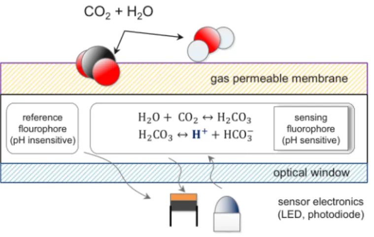
To reiterate, the optode foil is based on dual lifetime referencing (DLR) technique using two different fluorescent indicators (luminophores) embedded inside a gas per-meable polymer membrane coated on a sensor spot glass window. The first indicator is sensitive to changes in pH and responds with a change in the intensity of blue light-induced fluorescence. Because fluorescence intensity is sensitive to factors such as light (e.g. sampling is in the euphotic zone), a second reference indicator dye is in-corporated into the foil, not sensitive to pH with similar emission spectra, but much longer fluorescence lifetime compared to the pH-sensitive compound (Atamanchuk et al., 2014). When the sensing foil is excited by a pulsating blue light diode inside the optode, each indicator provides separate fluorescence signals. The two excitation responses have a phase lag (ϕDLR) used to determine CO2 concentrations through a

multi-point calibration model. The sensor foil was developed for Aanderaa, by Pre-Sens Precision Pre-Sensing Gmbh in Germany, similar to the well established O2 optode

models manufactured by ADI. The manufacturing quality of the sensor foil and cali-bration significantly influence the performance of the sensor, and great care must be

(37)

taken not to damage the physically and chemically sensitive foils.

For the CO₂ Optode, pCO₂ is related to phase shift and temperature through a multi-point calibration model (Atamanchuk et al., 2014), with an eighth-degree polynomial fit between sensor phase readings and temperature readings. The pub-lished method (ibid., 2014) requires 27 foil calibration coefficients (C(0,0) – C(8,3)) for

successfully calibrating the sensor to a range of oceanic conditions. The phase read-ings are also multiplied in a 3-degree polynomial with temperature to relate these to the temperature dependent polynomial coefficients (Ct0 – Ct8) for the fitted

phase-temperature pCO2 surface. Using the sensor phase angles (degrees), this yields the

base 10 logarithms of pCO2. All sensors, especially photo-chemical based, are known

to exhibit drift due to a conditioning period, as the sensors equilibrate to ambient conditions. Atamanchuk et al. (2014) suggest correcting any change in calibration model, for example, due to foil response drift, through subtracting a single reference point pCO_2,ref.

log(pCO₂) =Ct0 +Ct1 ×ϕ+...+Ct8 ×ϕ

8₋_log_(pCO

2,ref) (2.4)

We note that this fit model is arbitrary and other lower polynomial fits could be used, depending on how laboratory testing proceeds. Trying to fit the sensor to such a large number of inputs in temperature and molar CO₂readings requires a long testing time. Therefore, a lower number of calibration points would be desirable.

An issue with all sensors and in particular photochemical sensors is the impact of temperature on response time and ultimately sensor performance. Optode response time is typically slow compared to the speed of the glider. Gliders travel vertically at a speed of roughly 0.1 m·s−1. For a thermocline 5 m deep, with a temperature

(38)

gradient of 10◦C this would equal a temperature change of 0.2◦C·s−1, which could be to fast for the sensor foil chemistry to respond. These repeat temperature gradient inversions are difficult to resolve for low-power, non-pumped optodes, due to their strong temperature dependence, leading to additive errors over time unless the sensor is given a chance to equilibrate (e.g. through hovering at depth) (Bittig et al., 2014). Therefore, optode data from a moving platform require correction either through prior knowledge of the sensor response to temperature changes or through recursive data filtering. Another issue with foil chemistry on moving sensors is the impact of the boundary layer that invariably forms on the sensors as it transitions through the water column. Such a boundary layer will impact the sensor readings compared to the true ambient concentrations. The performance on gliders has been well characterized for Aanderaa oxygen optodes. For example, Bittig et al. (2014) investigated the impact of the boundary layer thickness on the response time of the sensor. Methods for drift correction during long deployments on Apex floats have also been published (Bittig and K¨ortzinger, 2015). For the CO2 optode, such information and characterization

are lacking, requiring each user to come up with their strategy to account for all the potential data quality issues during any deployment.

2.5.2 NDIR Gas Analyzer

The Pro Oceanus CO2-Pro CV is an example of a non-dispersive infrared refraction

(NDIR) based gas detector able to detect concentrations of molar CO2to the accuracy

of up to 1 ppm (parts per million) in air and water. The sensor has been developed for over a decade and has a patented system of chamber equilibration that collects

(39)

the gas pressure inside a special headspace and measures the absolute molar fraction (xCO₂) from the gas stream in ppm. The Pro CV offers an internal zero-reference measurement (ZM) to assess internal drift capability using Soda-Lime scrubbers to strip CO₂ from the gas stream and asses the internal drift of the infrared detector from zero CO2concentration. This capability is also present in the CONTROS Hydro

CTM and was used extensively in Fiedler et al. (2013) to quality control pCO2 data

from an autonomous float during post-deployment data processing. To compute the pressure of CO2 the gas chamber pressure and molar concentrations are multiplied.

pCO₂ = xCO2 ×Pheadspace (2.5)

Some instruments remove water vapour pressure and must be corrected for that, but the Pro CV already measures the wet gas stream, and therefore this correction is not necessary. It is recommended to use this type of sensor with a pump ensuring a constant supply stream of water into the sensing chamber of the instrument and shortening the time it takes for the sensor to equilibrate the internal and outside gas pressures.

The CO₂-Pro CV and Hydro C sensor has been assessed in numerous field studies and has known accuracy and stability (Jiang et al., 2014). This sensor, albeit accu-rate and reliable, has notable major drawbacks compared to the previously discussed optode sensor, limiting its portability on gliders. IR based colourimetry requires a lot more energy to detect IR wavelength absorption, compared to the optode lifetime signal detection. The sensor uses 4 W to operate (with a pump) and 9.5 W during the warm-up period, much too energy-demanding for a glider. Because of the gas stream equilibration, the sensor responds slowly to strong gradients in temperature and gas

(40)

pressure such as in profiling applications, requiring around 15 minutes with a pump to fully equilibrate to ambient xCO₂ conditions (Pro-Oceanus Systems Inc., 2018). For the Pro CV, in particular, some components of the sensor are fragile, and it is not known how well the sensor would function under constant profiling modes over months. Another issue with this sensor is the size (38 cm long with 10 cm diameter). The current sensors do not fit on gliders without some special adaption. In recent years Pro Oceanus manufactured a smaller version (28 cm and 5.1 cm diameter) of the CO2-Pro CV with lower power consumption: 0.4 – 0.6 W at 1 Hz rate without

pump (Pro-Oceanus Systems Inc., 2019), but still much more power demanding than the optode for comparison: 0.01 W at 1 Hz sampling rate. This sensor was experi-mentally tested on a glider in the Chukchi Sea (Hauri et al., 2018) and revealed long equilibration times (>1 min) and difficulty of employing current membrane technol-ogy glider for rapid profiling. By no means was this sensor modular within current glider payload capacity, requiring substantial modification of the vehicle to accom-modate the sensor and pump, impacting hydrodynamic efficiency. However, this type of sensor has started to see successful use in float based applications (Fiedler et al., 2013), and it is possible that in the near future this sensor will shrink even further in size. This could make this sensor relevant for glider applications, decreasing the equilibration time issue through the use of another reference instrument (e.g. pH or optode sensor) to approximate vertical CO2 gradients. It would be sufficient to use

the NDIR gas analyzer at select depths as calibration points and use the reference instrument to resolve depth profiles fully.

(41)

2.5.3 ISFET pH Sensor

Through the Wendy Schmidt Ocean Health X-PRIZE Competition, a new type of pH sensor was developed at Monterey Bay Aquarium Research Institute (MBARI) in collaboration with Honeywell, called the Deep-Sea ISFET pH Sensor. ISFET stands for Ion Sensitive Field Effect Transistor. This technology has been successfully used in collecting high accuracy data on profiling mooring in Monterey Bay (Johnson et al., 2016). This sensor was adapted for autonomous applications such as the APEX float by SeaBird Scientific called the Sea-Bird SeaFETTM_{, retaining the basic design}

from MBARI (Martz et al., 2010). The ISFET pH sensor works by measuring two different pH signals (external and internal) using the Durafet (Honeywell) solid state chloride selective electrode and an internal near perfect Nernstian response (salinity insensitive) reference electrode that is only temperature dependent (Takeshita et al., 2014). These two indicators have shown high stability in real oceanic test conditions (Bresnahan et al., 2014). In the presence of information on temperature and salinity from a CTD, the external electrode provides better accuracy (Miller et al., 2018) and can be used to assess internal drift of the sensor as is done in the integrated SeaBird SeapHOXTM _{CTD-DO-pH sensor package. The sensor has been available}

for purchase and integration to APEX floats by SeaBird. In total, about 200+ floats with this sensor have been deployed so far as part of the ongoing international ARGO programs such as Southern Ocean Carbon and Climate Observations and Modeling Program (SOCCOM) (Russell et al., 2014).

This sensor was recently tested on a glider as part of a study led by Dr Grace Saba between Rutgers University and SeaBird Scientific to monitor pH levels off

(42)

Atlantic City, NJ, USA. The sensor was integrated into the CTD of a 200 m Slocum Glider and over several weeks showed excellent characteristics under repeat 200 m profiling modes (Saba et al., 2018). During the study, the team focused on questions of sensor stability under repeat deployments, power consumption and issues around sensor calibration. The sensor output is a reference voltage that is converted into pH (total scale) using pressure, temperature and salinity information from the glider CTD using equations from Johnson et al. (2017). Using pH measurements, together with Total Alkalinity–Salinity (TA–S) relationships can be used to compute pCO2to

(43)

Chapter 3 Data and Method

3.1 Collected Data

As part of the Ventilations, Interactions and Transports Across the Labrador Sea (VITALS) project in 2016, two separate ocean observing platforms were deployed into the Labrador Sea: an underwater glider (deYoung et al., 2018) and a moored vertical profiler the SeaCycler (Send et al., 2013). These platforms resolve fundamentally different scales and ocean processes, but the deployment was designed to link these data sets together to provide better data about the spatial (glider) and temporal (SeaCycler) dynamics. A key aspect of the joint deployment was to use the glider in combination with SeaCycler to do in-situ tests and quality checks with a novel CO₂ optode sensor. Questions about the optode performance following inspection of the data from the Labrador Sea mission, led to more detailed glider based CO₂ optode testing in Trinity Bay in 2018. Here we describe the two deployments, including instrument setup and calibration and required processing to achieve a consistent data

(44)

set for further analysis and discussion in Chapter 4 and Chapter 5. Figure 3.1 shows various observing activities including SeaCycler, AR7W Stations, Glider T–S profiles for the Labrador Sea and Trinity Bay deployments.

3.1.1 Labrador Sea Deployment

As part of the VITALS program, a moored vertical profiler the SeaCycler (Send et al., 2013) and a G2 Slocum glider were deployed into the central Labrador Sea near the longtime German deep convection mooring K1. The K1 mooring, located about 25 km West of former OWS BRAVO (Avsic et al., 2006), has been deployed biennially since 1994 to monitor activity in the central deep convection patch in the Labrador Sea (Lavender et al., 2002). The objective of VITALS was to characterize the spatial and temporal structure of oxygen and CO2 in the deep convection zone.

Other research activities also took place in conjunction with VITALS, including a hydrographic section AR7W maintained by the Bedford Institute of Oceanography (BIO) and Argo floats released with several profiles captured near the SeaCycler site and the glider deployment area. Many coordinated observing efforts came together, utilizing multiple complimentary efforts across different scientific programs, relying on both traditional and novel observation approaches.

The SeaCycler was deployed near 52.22◦W and 56.82◦N, 30 km away from Ger-man deep convection mooring K1 (52.66◦W and 56.56◦N) to improve the vertical and time characterization of O2 and CO2 uptake in this region. The SeaCycler operation

and deployment techniques are in detail described in Send et al. (2013). Briefly, it is an underwater winch assembly, parked at 600 m depth with an instrument float that

(45)

Figure 3.1: Map of data collection sites.

can profile the top 150 m. A tethered communication allows for two-way telemetry over Iridium Satellite. Below the winch assembly, a single-point mooring line with instruments continues to the ocean depth of approximately 3500 m. For this deploy-ment, the instrument float carried CTD, ADCP and various gas sensors, including Clark-Type oxygen electrodes sensors (Seabird 41, Seabird 63), optodes (Aanderaa 4330 and CO2 Prototype 4797), Nitrate (Satlantic Deep Suna), Fluorescence,

Tur-bidity (Wetlabs) as well a bubble equilibrator infrared (IR) CO2 gas analyzer Pro

(46)

technol-ogy made by Pro Oceanus Ltd of Bridgewater, NS (Canada). Previous tests with this sensor showed excellent stability in multi-month vessel-underway missions (Jiang et al., 2014). The instrument float collected data over the top 150 m of ocean depth with 0.3 m vertical resolution from June 2016 to May 2017, while the Pro CV was sampling for 20 minutes at select stop depths (10, 30, 60, 120 m) to allow equilibration with ambient seawater pCO2. These stops resembled bottle stops done from ships

to calibrate new sensors. The K1 mooring was also equipped with oxygen sensors to allow for later cross mooring comparisons.

In the Fall of 2016, a Slocum G2 (generation 2) glider (Unit 473) was deployed from the Labrador shelf to reach the K1 SeaCycler site and complete 30 to 100 km long transects between moorings, collecting high-resolution spatial data. The glider was launched near Cartwright, Labrador from a small fishing boat and reached the deep convection zone near K1 and SeaCycler early in October, sampling there un-til 22 November. In total, the glider completed 18 full transects collecting valuable hydrographic and gas data. The modified glider with an extended battery bay car-ried two optical gas sensors in addition to a SeaBird glider CTD: a novel Aanderaa Data Instruments (ADI) CO2 optode prototype sensor (model 4797) described in

Atamanchuk et al. (2014), reviewed in Chapter 2, and the well established Aanderaa oxygen Optode (model 4831, SN 333). The CO2 optode (SN57) was equipped with a

thicker slow response foil based on the recommendation we received (D. Atamanchuk,

personal communications) to enhance long deployment stability. These sensors were mounted in the aft cone of the vehicle. Also, a thruster was installed to speed up the crossing of the shelf and to enable staircase profile sampling. The glider sampled the central Labrador Sea deployment location for two months, limiting CO2 optode

(47)

profiles to the top 200 m to save energy. In December, the glider began its journey back to Newfoundland following the 1500 m isobath inside the Labrador Current and reaching Trinity Bay (see map) on December 31, 2016. The glider was flown along the shelf break to take advantage of the southward flowing Labrador Current. Before deployment on the glider, the O2 and CO2 optodes underwent rigorous testing at the

biogeochemical laboratory facility at Dalhousie University to determine the calibra-tion model fit for the optode sensor foils. Bottle samples were collected during the deployment of the glider to compute offsets for the glider’s conductivity cell and any initial offsets for the glider optodes.

3.1.2 Trinity Bay Tests

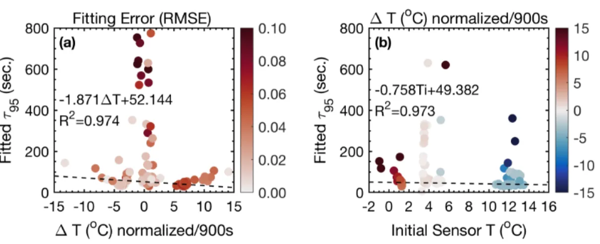
After completion of the VITALS mission, not confident that the mission had tested all the characteristics of the new CO2 sensor under glider profiling tests and in light

of emerging requirements for ocean carbon observatories, we conducted further tests of the optode on a glider to learn more about the sensor. Trinity Bay, Newfoundland, a deep inlet (up to 600 m in the Eastern part), easily reached by boat from numerous coastal communities was chosen as a test site. It is fed primarily by the cold Labrador Current waters and river runoff from the western side making it’s surface waters fresh and deeper portions frigid and highly oxygenated and nutrient-rich. The pooling of water in the deeper portion and surface freshwater produces a stable density stratifi-cation (Schillinger et al., 2000; Tittensor et al., 2002). Especially interesting for our optode tests are the large temperature gradients in the vertical of over 14◦C between the surface and 75 m depth. Trinity Bay has a cold water lens −1◦C between 70 m to

(48)

200 m depth, and temperatures below 1◦C from 200 m to the bottom. In Trinity Bay profiling through this lens leads to absolute temperature gradients of 10◦C or more, in 200 seconds or less.

Figure 3.2: (a) Trinity Bay test reference CTD, (b) glider setup and (c) equipment tank testing in progress.

We re-deployed the glider with the same CO₂ optode sensor from the Labrador Sea mission, in Trinity Bay in September 2018 for 12 days. The glider sampled the same properties as in the Labrador Sea mission CO₂ optode sensor (SN57) with the same foil as well as another CO₂ Optode sensor (SN56). During the deployment, it was quickly realized that this sensor, which had the thinner fast response foil, was very unstable, and data was corrupted and was noisy. The encountered problems with the thin-foil are consistent with experiences by other research groups (S. Borisov and F. Peeters,personal communications). Therefore, we omit this data from the ensuing

Glider-based O₂ and CO₂ observations in the Labrador Sea

Glider-Based O

and CO

Observations in the

Labrador Sea

Abstract

Acknowledgements

Contents

List of Figures

Chapter 1

Introduction

1.1

Motivation for this Thesis

1.2

Marine CO

and Carbon Observing Needs

1.3

The VITALS Program

1.4

Chapter Overview

Chapter 2

Background

2.1

Labrador Sea

2.1.1

Geography

2.1.2

Circulation

2.1.3

Convection

2.1.4

Labrador Sea and the CO

Sink

2.1.5

Wind-Driven Air-Sea CO

Flux Models

2.2

Implications of Labrador Sea CO

Uptake

2.3

Measurable Marine CO

Parameters

2.4

Gliders used for Labrador Sea Observing

2.5

Mobile in-situ CO

Sensors

2.5.1

CO

Optode

2.5.2

NDIR Gas Analyzer

2.5.3

ISFET pH Sensor

Chapter 3

Data and Method

3.1

Collected Data

3.1.1

Labrador Sea Deployment

3.1.2

Trinity Bay Tests