Mitigating Multi-Tenancy Risks in IaaS Cloud Through Constraints-Driven Virtual Resource Scheduling

(1)

Mitigating Multi-Tenancy Risks in IaaS Cloud Through

Constraints-Driven Virtual Resource Scheduling

Khalid Bijon

Institute for Cyber Security Univ of Texas at San Antonio

Ram Krishnan

Ravi Sandhu

ABSTRACT

A major concern in the adoption of cloud infrastructure-as-a-service (IaaS) arises from multi-tenancy, where multiple tenants share the underlying physical infrastructure oper-ated by a cloud service provider. A tenant could be an enter-prise in the context of a public cloud or a department within an enterprise in the context of a private cloud. Enabled by virtualization technology, the service provider is able to min-imize cost by providing virtualized hardware resources such as virtual machines, virtual storage and virtual networks, as a service to multiple tenants where, for instance, a tenant’s virtual machine may be hosted in the same physical server as that of many other tenants. It is well-known that separa-tion of execusepara-tion environment provided by the hypervisors that enable virtualization technology has many limitations. In addition to inadvertent misconfigurations, a number of attacks have been demonstrated that allow unauthorized in-formation flow between virtual machines hosted by a hyper-visor on a given physical server. In this paper, we present attribute-based constraints specification and enforcement as a mechanism to mitigate such multi-tenancy risks that arise in cloud IaaS. We represent relevant properties of virtual resources (e.g., virtual machines, virtual networks, etc.) as their attributes. Conflicting attribute values are specified by the tenant or by the cloud IaaS system as appropriate. The goal is to schedule virtual resources on physical resources in a conflict-free manner. The general problem is shown to be NP-complete. We explore practical conflict specifica-tions that can be efficiently enforced. We have implemented a prototype for virtual machine scheduling in OpenStack, a widely-used open-source cloud IaaS software, and evaluated its performance overhead, resource requirements to satisfy conflicts, and resource utilization.

Categories and Subject Descriptors

K.6.5 [Management of Computing and Information Systems]: Security and Protection

Permission to make digital or hard copies of all or part of this work for personal or classroom use is granted without fee provided that copies are not made or distributed for profit or commercial advantage and that copies bear this notice and the full cita-tion on the first page. Copyrights for components of this work owned by others than ACM must be honored. Abstracting with credit is permitted. To copy otherwise, or re-publish, to post on servers or to redistribute to lists, requires prior specific permission and/or a fee. Request permissions from [email protected].

SACMAT’15,June1–3, 2015, Vienna, Austria.

Copyright⃝c 2015 ACM 978-1-4503-3556-0/15/06 ...$15.00. DOI: http://dx.doi.org/10.1145/2752952.2752964 .

General Terms

Security

Keywords

Cloud IaaS; Virtual-Resource Scheduling; VM Migration; Multi-Tenancy; Constraint; VM Co-Residency Management

1. INTRODUCTION

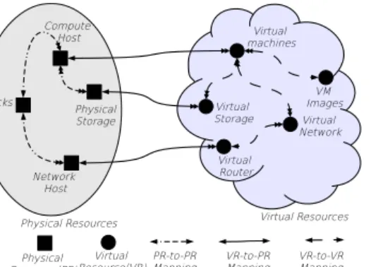
Enterprises are increasingly driven by economics and flex-ibility to utilize computing resources provided by cloud infr-astructure-as-a-service (IaaS) [32]. A major impediment to wider adoption of cloud IaaS stems from an enterprise’s loss of direct control over their virtual resources in cloud IaaS relative to the customary level of control over physical (or virtual) resources in an enterprise-managed data center [22]. In cloud IaaS, the physical resources in a datacenter are logically arranged by the cloud service provider (CSP) and virtual resources are hosted on those logical collections of physical resources. This is illustrated in figure 1 where a rack, for example, is a collection of a specific set of physical servers and network hosts. Other resources such as physi-cal storage volumes may be associated with those compute hosts in the rack. This is shown as physical resource to phys-ical resource mapping (PR-to-PR) in the figure. The single and double-headed arrows indicate the usual “one-to” and “many-to” mappings respectively. Tenants obtain a number of separate pieces of virtual computing resources (or sim-ply resources), e.g. virtual machines, virtual networks, etc., from the CSP. The cloud IaaS system should have suitable policy specification capabilities so that tenants can dynam-ically manage and arrange these resources to build a par-ticular computing environment based on their needs. For instance, tenants can systematically control specific virtual hardware (e.g. RAM, disk) assignment to virtual machines based on certain properties (e.g. purpose, running work-load type, sensitivity). This is shown as virtual resource to vir-tual resource mapping (VR-to-VR) in the figure and several mechanisms have been proposed [10, 11] to manage it.

More significantly, in cloud IaaS, physical hardware is also shared by multiple virtual resources for maximizing utiliza-tion and reducing cost. IaaS public or community cloud providers allow multi-tenancy which multiplexes virtual re-sources of multiple enterprises upon same hardware. This in-cludes co-location of virtual machines from different tenants on a single physical host, sharing physical disk storage, etc. This is illustrated as virtual resource to physical resource mapping (VR-to-PR) in figure 1. This raises many

(2)

secu-Figure 1: Cloud Resources Mapping Relation rity and performance considerations for a tenant’s workload in the cloud. For instance, a tenant’s virtual machines can be attacked by co-located malicious virtual machines of an adversary tenant. Similarly, highly cpu-intensive co-located virtual machines may disrupt each other’s expected perfor-mance. The work of Ristenpart et al [31, 36, 40, 41] has demonstrated such co-location vulnerabilities in real-world clouds. In particular, they show that preventing targeted co-location of virtual machines from diﬀerent tenants on the same physical server is unlikely to be successful. Their con-clusion is that “the best solution is simply to expose the risk and placement decisions directly to users” (i.e. tenants) [31]. The main objective of this paper is to address this goal where the tenants and the cloud system are able to schedule virtual resources on the physical resources consistent with high-level and ﬁne-grained constraints.

In this respect, even the leading IaaS service providers of-fer minimal support to their tenants. In particular, tenants have very little influence in how their resources are sched-uled. Of course, certain coarse-grained and static prefer-ences for disaster management are supported. For instance, the Amazon Web Services cloud infrastructure is hosted at multiple locations worldwide where a location comprises of multiple geographically isolated datacenters called a ‘Re-gion’ [1]. Each ‘Re‘Re-gion’ also has multiple, isolated locations known as ‘Availability Zones’. As a client, a tenant can at best specify the ‘Availability Zone’ of its virtual resources and specify backup Availability Zones for a premium. This concerns engineering for fail-safety but does not concern co-location of a tenant’s resources with those of others in a given physical server or a rack. This article explores a highly dy-namic and fine-grained technique for scheduling virtual re-sources based on high-level constraints specified by tenants in order to mitigate security threats (several of which are discussed in [5]) due to the co-residency of virtual resources. We present the design, implementation, and evaluation of an attribute-based constraints specification framework which enables tenants to express several essential properties of their resources as attributes and to specify values of those attributes that conflict for the purpose of co-locating vir-tual resources on a given physical resource. A constraints enforcement engine schedules virtual resources on the phys-ical resources while respecting the conflicts specified using attributes of those resources. For instance, consider two at-tributes of a virtual machine: atenant attribute that rep-resents the owning enterprise of that virtual machine, and a

sensitivityattribute that represents the sensitivity level of the data processed by that virtual machine. An example of

a high-level co-location constraint is that virtual machines of diﬀerent tenants may co-locate in a physical server as long as

thesensitivityis not ‘high’. As we will see, enforcing

con-straints in general in large-scale systems such as IaaS cloud is computationally ineﬃcient. Moreover, it negatively im-pacts physical resource requirements and their utilization— directly impacting the bottom line of IaaS CSPs.

The contributions of this paper are summarized below which aligns with its general outline.

•We present a design of an attribute-based framework for specifying co-location constraints of virtual resources sched-uled on given physical resources (section 2).

• Given that co-location constraints can drastically affect physical resource utilization, we propose a host optimiza-tion process while enforcing constraints (secoptimiza-tion 3). Note that, host optimization (i.e., optimizing the number of hosts necessary for scheduling thevms in a conflict-free manner) is an important requirement for achieving energy-efficient datacenter which is also a major concern for the CSPs for cost optimization [7]. We establish that, in general, the algo-rithms for host optimization while enforcing such constraints are NP-Complete (section 3). We demonstrate a subset of attribute conflicts that are of practical significance in varied application domains and cloud deployment scenarios (pub-lic, private, community, etc.), which can be efficiently en-forced in polynomial-time (section 3).

• We develop a prototype of the conﬂict-free virtual ma-chine scheduling framework in OpenStack [3] and rigorously evaluate the framework on various aspects, e.g., resource re-quirements, resource utilizations, etc. (section 4).

We analyze issues that arise due to the incremental changes of conﬂicts over time. A discussion of the security risks in this approach, some related works and conclusion are given in section 6, 7 and 8 respectively.

2. CONFLICT-FREE VIRTUAL RESOURCE

SCHEDULING

Intuitively, an attribute captures a property of an entity in the system, expressed as a name:value pair. In the context of cloud IaaS, attributes can represent a virtual machine’s owner tenant, sensitivity-level, cpu intensity-level of work-loads, etc. For simplicity, we restrict the scope of the paper as follows. We confine our attention to virtual to physical resource mapping in the context of virtual machines and physical compute servers. Then we briefly discuss the possi-ble extension of this approach to other virtual and physical resources. In the rest of the article we refer to physical com-pute host and virtual machine ashostandvmrespectively. We restrict the kind of constraint to “must not co-locate” constraint where the specified conflicts are co-location con-flicts that state whether twovms can be co-located in the same host or not. In this section, we formally define the components ofhosts allocation for thevms, which we refer as

host-to-vmallocation, in the presence of various co-location conﬂicts. Note that, avmmay have multiple attributes each with its own values. Attribute value of avmcan be assigned either manually by a user or automatically by the system. For instance, when an enterprise user creates avm, an

(3)

ap-propriate value is assigned to the tenant attribute of the

vm automatically whereas, the user may need to explicitly specify the value for a sensitivity attribute based on sen-sitivity of data processed in that vm. Developing adminis-tration models for such attribute assignments is beyond the scope of this paper. We assume thatvms are assigned with proper attribute values. For our purpose, the values of an attribute can conflict with each other and the goal is to al-low thevms to co-locate in same hostonly if their assigned attribute-values do not conflict. For general and in-depth understanding about various types of attribute conflicts we suggest to read the articles of Bijon et al [8, 9].

2.1 Scheduling Components Specification

The scheduling components include two sets calledHOST andVMthat contain the existinghosts andvms respectively. There are attributes ofvmthat characterize different proper-ties of avmand are modeled as functions. For each attribute function, there is a set of finite constant values that repre-sents the possible values of that attribute. For our purpose, we assume values of attributes to be atomic.1 Therefore, for a particularvm, the name of the attribute function maps to one value from the set. For convenience attribute functions are referred to as attributes. Also, values of an attribute can have conflicts with each other and these conflicts are speci-fied in a conflict-set of the attribute. Conflicts are specispeci-fied on values of each attribute independent of other attributes. Formally these components are defined as follows.

• HOSTis the ﬁnite set ofhosts (physical servers).

• VMis the ﬁnite set ofvms.

• Eachhost ∈ HOST has a capacity, represented as a function calledWHOST, that maps a hostto a value

greater than 1.0 to a maximum value of thehost ca-pacity2. The capacity restricts the number ofvms that ahostcan contain based on the accumulated capacity of the vms. Value of it for a host remains constant unless explicitly modiﬁed, e.g., increasing RAM size.

• Similar to the capacity of host, eachvm ∈VM has a capacity represented by a function calledWV M where,

WV M : VM→k where 0.0<k≤1.0. Also, capacity

of avmremains constant unless explicitly modiﬁed.

• ATTRVMis the set of attribute functions ofvm.

• For eachatt ∈ATTRVM, the domain of the function is

theVMand the codomain is the values ofatt written asSCOPEattwhich is a set of atomic values. Formally,

att: VM →SCOPEatt, for eachatt ∈ATTRVM.

The values inSCOPEattof anatt ∈ATTRVMthat conﬂict

with each other is speciﬁed as a relation called ConSetatt. 1

An example of an atomic attribute issensitivity where the values are high, medium and low. Avmcan only get one of the three values forsensitivity. However, some cases might require set-valued attributes for which avm may take mul-tiple values. For our purpose, we only consider atomic at-tributes, however, it can easily extend to set-valued one.

2

Multi-dimensional weights of a host, e.g., RAM, CPU, can be reduced to one single normalized weight. In Open-Stack [3],hosts are mapped to a single weight which is cal-culated by the weighted sum method that takes weighted average of diﬀerent metrics of ahoste.g., RAM, workload.

ConSetatt is reﬂexive and symmetric, but not transitive.

Hence, each element inConSetattis an unordered pair. For

eachatt ∈ATTRVM,ConSetattis deﬁned as follows. • ConSetattis the set of conﬂicts of the values of eachatt

∈ATTRVM. Formally,

ConSetatt⊆ {{x,y} |x̸=y and x,y∈SCOPEatt}

Part I in figure 2 shows two attributes,tenant and sensi-tivity, and their respective scopes. Some conflicts among val-ues oftenant andsensitivity attributes are also shown rep-resenting conflicts among their values. For instance,{{tnt1,

tnt2},{tnt2,tnt3}, {tnt4, tnt6}}inConSettnt speciﬁes that vms of tnt1and tnt2, tnt2and tnt3, and tnt4and tnt6conﬂict

with each other and, hence, cannot be co-located. Also, part IV shows an example of attribute assignment forvms. For instance, for vm1,tenant(vm1) = tnt3andsensitivity(vm1)

= high. Also note that the value 0.6 denotes the capacity requirement of thatvm. That is,WV M(vm1)=0.6.

2.2 Conflict-Free Host to VM Allocation

Given that theConSetattspeciﬁes conﬂicting values for an

attributeatt ∈ATTRVM, the conﬂict-freehosttovm

alloca-tion is concerned about allocaalloca-tion of ahost to a group of

vms that do not conﬂict with each other. There are 4 steps in this process as illustrated in ﬁgure 2. Step 1 is to par-tition the values of each attribute (i.e.,SCOPEattof anatt ∈ATTRVM), into a family of subsets where the elements in

each subset do not conﬂict with each other. We refer to such partitionas “Conﬂict-Free Partition of Attribute-Values”.

Definition 1. (Conflict-Free Partition of

Attribute-Values)Aconﬂict-free partition of attribute-valuesof each att ∈ ATTRVMis speciﬁed as PARTITIONatt that partitions

the values inSCOPEattwhere the values of each element in

PARTITIONattdo not conﬂict with each other, i.e., for each

x∈PARTITIONattand for each y∈ ConSetatt,|x∩y| ≤1

We can state that, for an attributeatt, aPARTITIONatt

partitionsSCOPEattwhere (1)PARTITIONattdoes not

con-tain∅, (2) elements inPARTITIONatt are pairwise disjoint,

(3) the union of the elements inPARTITIONattisSCOPEatt,

and (4) the values in a set-element ofPARTITIONattdo not

conﬂict with each other, i.e. no more than one value from that set-element belongs to the same element inConSetatt.

Part II in ﬁgure 2 shows examples of conﬂict-free parti-tions,PartitiontenantandPartitionsensitivity, forConSettenant

and ConSetsensitivity given in part I. For example, {tnt1,

tnt3, tnt6}inPartitiontenantmeans these values do not

con-ﬂict with each other. Note that, there can be multiple candi-datePARTITIONattfor a givenConSetattof an attributeatt ∈ATTRVM. Section 3 shows that the selection of an

appro-priatePARTITIONattis important for the host optimization.

Step 2 combines the conflict-free partitions of attribute-values of all attributes. We define a conflict-free segment that consists one element ofPARTITIONattof each attribute

att ∈ ATTRVM. We will see later that vms, mapped to a

conflict-free segment, do not conflict with that of others, hence, can co-locate. Note that avmcan get any value from the scope of an attribute. Therefore, conflict-free segments should be generated in such a way so that it can map all pos-sible assigned values to the attributes of thevms. A cartesian product of thePARTITIONattfor allatt∈ATTRVMgenerate

all possible segments of conﬂict-free values of the attributes that can avmbased on its assigned attribute values.

(4)

Figure 2: Conﬂict-Freevm-hostAllocation

Definition 2. (Conflict-Free Segments of the

Val-ues of Attributes)Theconﬂict-free segments of the values of attributes is a set, called ConflictFreeATTR, of n-tuples where n =|ATTRVM|and each tuple is a result of the carte-sian product of PARTITIONatt of all att ∈ ATTRVM, i.e.,

ConflictFreeATTR= ∏

att∈ATTR_VM

PARTITIONatt

Each elementconF val∈ ConflictFreeATTRis an ordered pair which is written as⟨Xatt1, ..., Xattn⟩ where{att1, ...,

attn}=ATTRVM and Xatti ∈PARTITIONatti. We assume

that elements of each conF val ∈ ConflictFreeATTRcan be accessed by the notationconF val[att] for eachatt∈ATTRVM.

Part III in ﬁgure 2 shows an example ConflictFreeATTR which is produced from the Cartesian product of conﬂict-free partitionsPartitiontenant andPartitionsensitivity. A

tu-ple ({tnt1, tnt3, tnt6},{high}) is an element in

Conflict-FreeATTR since{tnt1, tnt3, tnt6}and {high}are members

of PartitiontenantandPartitionsensitivityrespectively.

Step 3 partitions the setVMsuch thatvms of each element of the partition can be co-located. This is achieved by parti-tioningVMin a way such that each element of the partition can be mapped to an element of ConflictFreeATTR.

Definition 3. (Co-Resident Partition of VM) The

Co-Resident Partition of VM, speciﬁed as CoResidentVM-Grp, is a partition ofVMwhere the assigned values to att ∈

ATTRVMof allvms in an element of the partition map to the same segment inConflictFreeATTR, i.e.,

for all X_∨∈ CoResidentVMGrp and for all vmi̸=vmj ∈ X, conFval∈ConflictFreeATTR

SetResidence(vmi, vmj, conFval,ATTRVM))

where, SetResidence(vm_∧ i, vmj, conFval, ATTRVM) = att∈ATTRVM

(att (vmi)∈conFval[att ]∧att (vmj)∈conFval[att ])

CoResidentVMGrp partitions VM if vms in an element of CoResidentVMGrp are assigned to the values, for all att ∈ ATTRVM, that belong to the same element inConflictFreeATTR.

Part IV in figure 2 shows an example of CoResidentVM-Grp calculation of 10vms where vms are mapped to differ-ent elemdiffer-ents ofConflictFreeATTRbased on their attributes. For instance, vm1 is mapped to the segment ({tnt1, tnt3,

tnt6},{high}) since it is assigned with ‘tnt3’ and ‘high’ for

tenant and sensitivity attributes. Also, vm1 and vm3 be-long to the same partition of CoResidentVMGrpsince they are both mapped to the segment ({tnt1, tnt3, tnt6},{high}).

Finally, step 4 allocateshosts for thevms of each partition inCoResidentVMGrp. Ahostcannot containvms from mul-tiple partitions ofCoResidentVMGrp. Also, combined capac-ity of the allocatedvms must satisfy the capacity (WHOST)

of thehost. Therefore, for each partition of vms in CoResi-dentVMGrp, multiplehosts might be required depending on the combined weight of thevms in that partition.

Definition 4. (Conflict-Free Host to VM

Alloca-tion)GivenVM,HOST,ATTRVM,CoResidentVMGrp, WHOST

and WV M, the Conﬂict-Free Host to VM Allocation is a

mapping function called allocate that ﬁnds a set of hosts,

HOST′ ⊆ HOST, to allocate all vm ∈ VM where the vms that reside in ahostform a subset of an element of CoResi-dentVMGrpsuch that their combined weight does not exceed the weight ofhost, i.e., allocate : HOST′ ,→ P(VM) where, if chost∈HOST′ and allocate(chost) = lvm, then,

lvm⊆VM∧ ∨

x∈CoResidentVMGrp

lvm⊆x∧( ∑

vm∈lvm

WV M(vm))≤WHOST(cs)

Part V in ﬁgure 2 shows an example of Conﬂict-Free Host to VM Allocation where the total number ofvms is 10 and they are partitioned into 4 co-resident sets. Note that, here,

(5)

Host0 and Host1 are allocated to one co-resident partition of vms containing {vm0, vm1, vm3} since their combined weight is more than the weight of a singlehost.

2.3 Conflict-Free Scheduling of Other Virtual

Resources to Physical Resources

The process of sections 2.1 and 2.2 can also apply for the scheduling of other virtual resources (shown in ﬁgure 1) with the following modiﬁcations.

In physical storage to virtual storage allocation, two sets VM and HOST, defined in section 2.1, are substituted by sets VS and PS that specifies virtual storage volumes and physical volumes in the system respectively. Similar to the capacity functions ofvmandhost, two functions can be de-fined for virtual and physical resources that can map their respective capacities where the capacity can be a single met-ric calculated by weighted sum of different properties of a storage system. Such properties include size, storage i/o speed, etc. Now, similar to the ATTRVM, a set can

rep-resent the attributes of the virtual storage volumes. Also, ConSetattand deﬁnition 1-4 can be modiﬁed accordingly for

the physical storage to virtual storage allocations.

A similar approach can be followed to derive the network host to virtual router allocation. Here, two sets calledNH andVRcan specify network hosts and virtual routers in the system respectively. Now the capacity could be the limit of network bandwidth of a network host and the bandwidth of a virtual router. One motivation of scheduling virtual router across different network hosts is for load-balancing of the network traffic and ensuring availability. Here, similar to the virtual machines, necessary attributes of the virtual routers can be generated. ConSetattand definition 1-4 can

be modiﬁed for network host to virtual router allocations.

3. OPTIMIZATION PROBLEM DEFINITION

AND SOLUTION ANALYSIS

In this system, the specified conflicts restrict certainvms from co-locating in the samehost. Hence, somehosts can-not schedulevms that conflict with currently scheduledvms in thesehosts, despite having the required capacity. That in-creases the required number of hosts than a system without conflicts. Hence, it is desirable to schedulevms in a way that minimizes the number ofhosts while satisfying the conflicts leading to an optimization problem.

Definition 5. (Host Optimization Problem)TheHost

optimization problemseeks to minimize the number ofhosts in the mapping, allocate : HOST′ ,→ P(VM), specified in Conflict-Free Host to VM Allocation (Definition 4).

This section investigates algorithms for deﬁnition 1 through 4 in order to solve the Host Optimization Problem.

3.1 MIN PARTITION: Minimum Conflict-Free

Partitions of Attribute-Values

More than onePARTITIONattcan be generated for a given

ConSetatt. In ﬁgure 2, for the givenConSettenant, candidate

Partitiontenantsets could be{{tnt1, tnt3},{tnt2, tnt6},{tnt4,

tnt5}}and{{tnt1,tnt3,tnt6},{tnt2,tnt4,tnt5}}with 3 and 2 elements in the sets respectively. Here, each element of a PARTITIONattcontains the conﬂict-free attribute-values of

att. Number of elements inPARTITIONatt aﬀects the total

number of conﬂict-free segments (deﬁnition 2) where thevms

mapped to same conﬂict-free segment can co-exist. A parti-tion, with minimum number of elements, reduces the num-ber of conﬂict-free segments. It also reduces the elements in CoResidentVMGrpthat also minimizes the required number of hosts. We call such a partition asMIN PARTITION.

Finding aMIN PARTITIONis similar to the graph-coloring problem that partitions the vertices of a graph G(V,E) into minimum color classes so that no two adjacent vertices, such as{v1,v2} ∈E, fall in the same class. Graph-coloring prob-lem is NP-Complete given that graph coloringdecision prob-lem, called k-coloring, is NP-Complete, which states that given a graph G(V, E) and a positive integer k≤ |V|, can the vertices in V be colored by k diﬀerent colors?

We show thatMIN PARTITIONis NP-Complete by show-ing that the MIN PARTITIONdecision problem, which we refer to as K PARTITION, is NP-Complete. The problem states that givenSCOPEattandConSetattof anatt∈ATTRVM,

and a positive integer k ≤ |SCOPEatt|, can the values in

SCOPEattbe partitioned into k sets?

Theorem 1. K PARTITIONis NP-Complete.

Proof. We prove thatK PARTITIONis NP-Complete by polynomial-time reduction of k-coloring toK PARTITION.

Aninstance of k-coloring is a graph G(V, E) and an in-teger k. We construct SCOPEatt ←V and ConSetatt ←E

and feedSCOPEatt,ConSetatt, and k toK PARTITION. The

complexity of this conversion is|V| × |E|.

Now we show that anyes instanceof k-coloring maps to anyes instance of K PARTITIONand vice versa.

=⇒ Assume G is an yes instance of k-coloring and there exists a set of colors C of size k in G. Thus, for all u∈V, color(u)∈C and for any u, v∈V, color(u)=color(v) only if

{u, v} ̸∈E. Also, for all u∈ SCOPEatt, u belongs to cfs∈

CFS where #CFS is k, and for any u, v∈SCOPEatt, u, v

belongs to the same cfs∈CFS, if{u, v} ̸∈ConSetatt. Thus,

G is anyes instance of K PARTITION.

⇐= AssumeSCOPEatt,ConSetattis anyesinstance of

K PARTITION and there exists a family of CFS of size k. Thus, for all u∈ SCOPEatt, u belongs to a cfs∈CFS, and

for any u, v ∈ SCOPEatt, u, v belongs to the same cfs ∈

CFS, if{u, v} ̸∈ ConSetatt. Thus, the vertices in same cfs ∈CFS can be colored by the same color and there will be k number of colors to color all the vertices in G. Thus, G is anyes instance of k-coloring.

Thus,K PARTITIONis NP-Complete.

Therefore, MIN PARTITION is also NP-Complete. How-ever, there are a number ofapproximate graph-coloring al-gorithms that can be applied toMIN PARTITION. The algo-rithms are approximate in the sense that they may not pro-vide the minimum size ofPARTITIONatt, i.e.,MIN PARTITION

may not be optimal. This is useful, although not optimal, because the conﬂicts are still satisﬁed. In appendix A, we discuss approximate algorithms for graph-coloring and their applications to MIN PARTITION. We also develop an ex-act algorithm, shown in algorithm 1, based on backtrack-ing. The complexity of this algorithm is NP since it is an adaptation of the general backtracking algorithm for the graph-coloring [6]. However, for attributes whose size of the scope is small enough (e.g. sensitivity), the algorithm computes the partition relatively fast. In algorithm 1, the MAKE PARTITION procedure is called with scopeSCOPEatt

(6)

Algorithm 1Conﬂict-Free Partition using Backtracking 1: procedureCheck Validity(attval,ConSetatt, CSet)

2: for allattvali∈CSetdo

3: if {attval, attvali} ∈ConSetattthen

4: Return False

5: end if

6: end for

7: Return True

8: end procedure

9: procedure _{Make Partition}(SCOPEatt, ConSetatt,

PARTITIONk att)

10: if attval∈SCOPEattthen

11: for allpar∈PARTITIONkattdo

12: if CHECK VALIDITY(attval, ConSetatt,

par)then

13: par = par∪attval

14: if MAKE PARTITION(SCOPEatt-{par},

15: ConSetatt,PARTITIONkatt)then

16: Return True

17: end if

18: par = par−attval

19: end if 20: end for 21: end if 22: Return False 23: end procedure PARTITIONk

att that can contain k elements. It uses a

re-cursive backtracking algorithm that tries all possible com-binations ofk partitions and returns true if there is a valid conﬂict-freekpartition of a givenConSetatt. Before adding

an attribute value to a partition, MAKE PARTITION calls CHECK VALIDITY that veriﬁes if the attribute value to be added is indeed free of conﬂict with respect toConSetatt. In

section 4, we analyze the performance of this algorithm for various sizes of attribute scopes and conﬂict sets.

Certain graphs such as perfect graphs have polynomial graph-coloring solutions. We identify that certain restricted versions of attribute conflict specification generates such graphs. For example, like in a Chinese-Wall policy, an or-ganization can have a conflict-of-interest with certain other organizations. For instance, all banking tenants of a CSP may have a conflict-of-interest with each other. Similarly, all the oil-company tenants may conflict. ACSP can generate an attribute calledtenantthat represents a particular tenant name in the system, e.g, bank-of-america, and the values of tenant can be categorized into mutually disjoint conflict-of-interest classes. The conflict-set generates disjoint cliques of attribute values which can be solved in polynomial-time [18]. Appendix B discusses several such restricted conflicts.

3.2 ConflictFreeATTR Generation

This is a trivial algorithm that calculates the values of ConflictFreeATTR speciﬁed in deﬁnition 2. The algorithm takes as input PARTITIONatt for all att ∈ ATTRVM, and

returns ConflictFreeATTR which is a Cartesian product of PARTITIONatt for allatt. It also stores the calculated

or-dered tuples inConflictFreeATTR. The complexity isO(n× m) wherenandmare the size ofATTRVMandPARTITIONatt.

3.3 Co-Resident VM Partitions Generation

This algorithm takesConflictFreeATTRandVMsets as in-put, creates a family of sets, calledCoResidentVMGrp (deﬁ-nition 3), where each set contains a subset of vms that can co-reside. The number of sets inCoResidentVMGrpis equal

Figure 3: Experimental Setup in OpenStack to the number of elements inConflictFreeATTR, where the algorithm maps an element of ConflictFreeATTR to an el-ement in CoResidentVMGrpand the mapping is one-to-one and onto. Thevms that map to the same element in Conflict-FreeATTRbelong to the same partition. The complexity of this algorithm isO(VM × ConflictFreeATTR ×ATTRVM).

This algorithm works for both offline and online versions of VM scheduling. In offline, the total number of vms is fixed and are given before the algorithm runs. In online, the scheduling request for avm arrives one at a time. For both versions, the algorithm takes one vm and maps it to an element inConflictFreeATTRand adds thevmto a corre-sponding element inCoResidentVMGrp.

3.4 Scheduling VMs to Hosts

This algorithm takesCoResidentVMGrp, and schedules the

vms that belong to each element in CoResidentVMGrp, to-gether in one or more hosts. For vms of each element in CoResidentVMGrp, this process might need one or morehosts based on the combined capacity of thevms. If the total ca-pacity exceeds the caca-pacity of a singlehostthen it will need multiple hosts. This scheduling problem is similar to the bin-packing [16] problem which is NP-Hard. However, there are a number of known heuristic approaches that can be ap-plied here [30]. The scheduling of vms in an optimal way based on capacity is orthogonal to MIN PARTITIONsince MIN PARTITIONis solved before this scheduling begins.

4. IMPLEMENTATION AND EVALUATION

We implement and evaluate our conﬂict-free vm to host

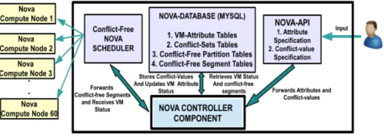
scheduling framework. Since our work concerns scheduling, to conduct realistic experimentation, we need exclusive ac-cess to a large-scale cloud infrastructure with 100s of phys-ical hosts to meaningfully study resource requirements and its utilization. First, we setup an IaaS cloud environment using a set of 5 physical machines (each of them is a Dell-R710 with 16 cores, 2.53 GHz and 98GB RAM). We now treat each of thevms that this cloud provides as a physi-cal host. Thesevms are conﬁgured with 4 cores and 3 GB of RAM. We now create a DevStack-based cloud framework [2], a quick installation of OpenStack ideal for experimentation, using thosevms as physical hosts to create a virtual cloud for the purpose of experimentation. Now, we create the second-level ofvms to get a virtual IaaS cloud and the conﬁguration of thesevms are varied based on the experiment we perform. We implemented ourhost-to-vmscheduling on the testbed described above. Figure 3 illustrates our experiment setup. In OpenStack, the component that takes care of vm man-agement and scheduling is the Nova service. We created a cloud cluster with 61hosts where one of them is the Nova controller node and another 60 are the Nova compute nodes.

(7)

(11,30,0.0056) (11,30,0.011) 12 ₁₅ 18 ₂₁ 24 ₂₇ 30 No. of Elements in Attribute Scope 20 24 28 32 36 40 No. of Elements in Conflict-Set 0 0.05 0.35 0.85 1.45 1.95 2.45 3 3.5 4 Time (Sec)

Figure 4: Required Time for Small Scope and Confilct-Set (50,70,416) 40 ₅₀ 60 ₇₀ 80 ₉₀ 100 No. of Elements in Attribute Scope 4050 6070 8090 100 No. of Elements in Conflict-Set 0 400 800 1200 1600 2000 2400 Time (Sec)

Figure 5: Required Time for Large Scope and Conflict-Set 0 0.05 0.1 0.15 0.2 0.25 0.3 100 200 300 400 500 600 700 800 900 1000 Ti me (sec) Number of Vms Conflict-Free VM Scheduler

Figure 6: Latency for Conflict-free Scheduling 0 2 4 6 8 10 12 14 16 18 0 20 40 60 80 100 120 140 160 Nu m b er of Se rv er s Cardinality of Conflict-Set Scheduling: 100 VMs 200 VMs 300 VMs

Figure 7: Required Number ofhosts for Varying

Number of Elements in Conflict-Set

0 2 4 6 8 10 12 14 16 18 20 22 24 26 6 9 12 15 18 Num b er of Ser v ers

Maximum Degree of Conflicts Scheduling: 100 VMs 200 VMs 300 VMs

Figure 8: Required Number of hosts for Max

Degree of Conflicts 0 10 20 30 40 50 60 70 80 90 100 20 40 60 80 100 120 140 160 180 200 Ser v er Uti li za ti o n (P er cen t a ge) Number of Vms Without Conflicts Max Degree-of-Conflicts 5 Max Degree-of-Conflicts 10 Max Degree-of-Conflicts 15 Max Degree-of-Conflicts 20

Figure 9: Host Utilization Overhead

The Controller node provides main services, e.g. database, message queues, etc., while the compute nodes only con-tain components such as hypervisor and nova-compute that are required for runningvms. We deployed the prototype in the nova controller node. Our python-based implementation of conflict specification allows tenant admins to specify at-tribute conflict values and the ability to store conflict values in nova database (MySQL) (part I in figure 2). Our python based conflict free segments calculation process (steps 1 and 2 in figure 2) has 153 lines of code. Finally, our implementa-tion of conflict-freehosttovmscheduling (steps 3 and 4 in figure 2) has 170 lines of code that maps avmto a conflict-free segment based on conflicting-values and assigned at-tribute values of the vmwhich are retrieved from the nova database. For the conflict-free segment, designated hosts are identified and weighed based on default Nova weighing factors and thevmis scheduled to the suitablehost.

Experiment 1 -Upper Bound of Algorithm 1. This

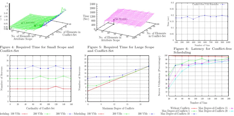
ex-periment analyzes the runtime of Algorithm 1. Since the complexity is in NP, here, we identify the maximum size of scope and conflict set for which required runtime of the al-gorithm remains feasible. First, we conduct the experiment with a small size of scope of an attribute and respective conflict set. We vary scope size from 10 to 40, and for each scope size, we vary the size of conflict set from 20 to 40. For each scope and a particular size of the conflict set, we randomly create elements in conflict set and execute the al-gorithm. Figure 4 shows the results where, for a small scope and conflict set, runtime is very low, e.g., 0.011s for a scope and conflict set size of 18 and 30 respectively. However, for bigger scope and conflict set sizes, it increases drastically, e.g, for scope size 30 and conflict set size 35 it becomes ap-proximately 4s. We also conduct the same experiment for

large scope and conflict sets where we vary the size from 40 to 100 and 60 to 100 respectively. Figure 5 shows the results where the runtime is very high as expected. For instance, for a scope and conflict set size of 50 and 70 respectively, the ex-ecution time is more than 7mins. Note that, a high runtime may be acceptable, since conflict-free partitions are created before starting the scheduling ofvms and hence it does not impact the scheduler’s performance drastically. This experi-ment gives an estimation of delay theCSPmight face before scheduling thevms if it wants to create conflict-free partitions for a given scope and conflict set size.

Experiment 2 - Scheduling Latency. In the second ex-periment, we analyzed the timing overhead of our conflict-free host-to-vm scheduler once that conflict-free partitions are calculated by algorithm 1. In figure 6, we study how the amount of time the scheduler takes to schedule a single

vmvaries with increasing number of vms that have already been scheduled. A value of 500 in the x-axis, for exam-ple, indicates that 499vms have already been scheduled and the corresponding value in the y-axis (0.19s) indicates the time to schedule one new vm. The attribute values of the pre-scheduledvms were randomly assigned. The scheduler takes a fairly ﬁxed amount of time to schedule a singlevm

regardless of the number of conﬂict-free pre-scheduledvms.

Experiment 3 - Required Number of Hosts. Our third

experiment concerns the impact of satisfying conflicts on the resource requirements. In our case, the conflict set of a given attribute can be varied in two significant ways to evaluate the number of physical hosts that are necessary. In figure 7, we vary the number of elements in the conflict set while fix-ing the maximum degree of conflict to a constant value. The highest number of values that conflict with each other in the conflict set is referred to as the maximum degree of conflict

(8)

for that conflict set. In figure 7, we fix the maximum degree to 2. In figure 8, we vary the maximum degree of conflicts with a fixed attribute scope. Given the server memory ca-pacity to be 3 GB, the vm capacity is varied between 512 MB and 1024 MB. The experiment confirms our intuition that that the maximum degree of conflict dominates the server requirement to schedulevms. Note that minor spikes and drops (for example between 100 and 140 on the x-axis for scheduling 100 vms) are due to the randomness of the workload we automatically generate and some variability in Devstack. However, overall, our observation holds true.

Experiment 4 - Host Utilization. Finally, this experi-ment concerns the impact of conflict-free scheduling on the overall utilization level of all the physical servers. Since we know from experiment 2 that resource requirements are pre-dominantly impacted by maximum degree, in figure 9, in the x-axis we vary maximum degree while scheduling a varied number of vms. The y-axis specifies the aggregate percent-age of utilization of all the servers after scheduling thevms in a conflict-free manner. For example, given N number of servers, 80% utilization means that 20% of N servers in total is not utilized. We can see, server utilization dramat-ically increases with the number of vms that are scheduled. This is because since the max degree dictates server require-ments, for smaller number ofvms, a minimum of max degree number of servers remain heavily under-utilized. Once the

vms scale toward real-world numbers, the utilization is above 80% even with a very high degree of conﬂict.

5. INCREMENTAL CONFLICTS

So far, our conflict-free scheduling approach has assumed that conflicts can be pre-specified and remains unchanged. However, in practice, conflicts may change, and may be spec-ified incrementally as new tenants join the cloud. We now explore this fundamentally hard problem—if two vms that did not conflict at a certain time happen to be co-located in a server, but later develop a conflict due to an update of conflict specification, it is necessary to migrate one of those

vms from that server, to remain conﬂict free.

5.1 Types of Conflict Change

In general, a conflict-set changes if a new conflict is added or an existing conflict is removed. Given aConSetattand a

PARTITIONattof anatt∈ATTRVM,ConSetattcan change to

a new conﬂict setConSet′att( a new partitionPARTITION′att

can be calculated accordingly) in three diﬀerent ways.

•∆1—this type of change involves operations that only

re-move an element from ConSetatt where |PARTITION′att|< |PARTITIONatt|. Evidently, it does not add new conﬂicts,

hence, the scheduledvms need not migrate.

•∆2—this type of change involves operations that add an

element toConSetatt. However,PARTITIONattremains

un-changed. If addition of a new conﬂict results in no change in conﬂict-free partition, scheduledvms need not be migrated.

• ∆3—this type of change adds an element to ConSetatt

where PARTITION′att̸= PARTITIONatt. Evidently, certain vms need to be migrated if they need to remain conﬂict-free. Consider an attribute att ∈ ATTRVM and SCOPEatt = {a1,a2,a3,a4,a5,a6}, where the initial conﬂict-setConSetatt

={{a1,a2},{a1,a4},{a2,a4},{a1,a5},{a2,a6},{a4,a6}}and the corresponding partition set which is calculated using

al-gorithm 1 isPARTITIONatt={{a1,a3,a6},{a2,a5},{a4}}.

Consider a change of type ∆1 that removes{a2,a4}

from ConSetatt where resultant conﬂict set ConSet1att={{

a1,a2},{a1,a4},{a1,a5},{a2,a6},{a4,a6}}andPARTITION1att

={{a1,a3,a6},{a2,a4,a5}}. Here, #PARTITION1att<

#PARTITIONattand it does aﬀect already scheduledvms.

Consider a change of type ∆2 that adds {a2,a3} to

ConSetattwhere new conﬂict setConSet2att={{a1,a2}, {a1,a4},{a2,a4},{a2,a3},{a1,a5},{a2,a6},{a4,a6}}and PARTITION2att={{a1,a3,a6}, {a2,a5},{a4}}which is equal

to the previous partition setPARTITIONatt.

Consider a change of type ∆3 that adds {a1,a6} to

ConSetatt where ConSet3att= {{a1,a2}, {a1, a4}, {a2,a4}, {a1,a5},{a2,a5},{a2,a6},{a4,a6},{a1,a6}}andPARTITION3

att

={{a1,a3},{a2},{a4},{a6}}. This clearly aﬀects the previ-ously scheduled VMs because, fromPARTITIONatt,vms with

attribute value a4 are co-located withvms with attribute val-ues a1 or a3. Now, thosevms with a4 need to migrate since they cannot co-locate with a1 or a3.

5.2 Cost Analysis

In this section, we analyze the cost of continuing to satisfy the conﬂicts as they change, when the change is of type ∆3.

We calculate the cost based on the number of migrations that are necessary when conﬂicts change. Based on experi-mentation, we gain insights on the strategies for minimizing the cost while handling this type of change.

We define an incremental plan, or simply plan, as a se-quence of operations that adds a number of conflicts to the current conflict-set resulting in a ∆3-type change (i.e.,

re-quires migration). Our strategy for minimizing cost is as fol-lows. Consider an element{a1, a2, a3, a4}of a conﬂict-free partition setPARTITIONattof attributeatt. Since attribute

valuesa1 througha3 are conflict-free, the scheduler is free to co-locatevms that have those attribute values in a given server. We refer to this aspromiscuousconflict-free schedul-ing because it maximizes the mixschedul-ing ofvms in a given server so long as they do not conflict. In contrast, aconservative approach minimizes the co-location ofvms even though their attribute values do not conflict. For instance,vms with val-uesa1 ora2 may be co-located in one server, and those with valuesa3 ora4 may be co-located in another. In this case, if valuesa3 anda1 were to develop a conflict in the future, the migration cost can be minimal (zero in this scenario). Promiscuous scheduling can have better resource utilization but higher cost for managing conflict changes. Conservative scheduling can minimize cost when conflict changes more frequently, at the expense of lower resource utilization.

We conduct an experiment to evaluate the impact of con-ﬂict change on the number of migrations for diﬀerent levels of conservative scheduling. The steps of the experiment are: (step-1)We consider a single vmattribute calledatt where we vary the size of SCOPEatt from 10 to 35 with an

incre-ment of 5. (step-2) For each SCOPEatt, initially, we

ran-domly populateConSetattwith 5 to 50 elements and

calcu-latePARTITIONatt. We repeatedly perform this step for 50

times for everystep 1. (step-3)For eachstep-2, we schedule X number ofvms where we vary X from 500 to 5000. We also schedule them using a promiscuous approach and four con-servative approaches where VMs of samehostcan not have

(9)

0 15 30 45

5 10 15 20 25 30 35 40 45 50

(A) Scheduling Process 1(Max. 2) Mean of Avg. Per.(%) of Migrations Mode of Avg. Per.(%) of Migrations

0 15 30 45

5 10 15 20 25 30 35 40 45 50

(B) Scheduling Process 2(Max. 4) Mean of Avg. Per.(%) of Migrations Mode of Avg. Per.(%) of Migrations

0 15 30 45

5 10 15 20 25 30 35 40 45 50

(C) Scheduling Process 3(Max. 8) Mean of Avg. Per.(%) of Migrations Mode of Avg. Per.(%) of Migrations

0 15 30 45

5 10 15 20 25 30 35 40 45 50

(D) Scheduling Process 4(Promiscuous) Mean of Avg. Per.(%) of Migrations Mode of Avg. Per.(%) of Migrations

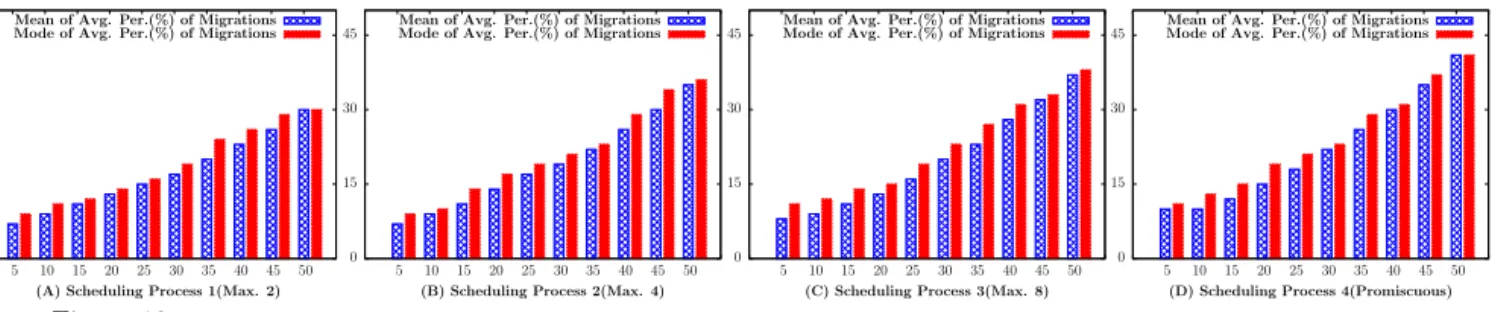
Figure 10: Cost Analysis: X-axis(% of the Total Conflicts for Given Scopes), Y-axis(% of Total VMs that Require Migrations)

more than 1, 2, 4, and 8 different values from a conflict-free partition respectively. Also, each vm is randomly assigned a value to its att. We repeat each scheduling process for 30 times. We also randomly assign vmmemory capacity to 512 and 1024 MB, andhostcapacity to 3GHz. (step-4) Fi-nally, we measure migrations for 5 differentplanswhere the plansgradually add random 5%, 10%, 15%, 20%, 25%, 30%, 35%, 40%, 45% and 50% of the total number of conflicts to ConSetatt respectively. For each plan,step-4 is repeated

for 50 times and we count the migrations. Note that these numbers (the number of times a particular step is repeated) provide suﬃcient variations, and are primarily dictated by amount of time it takes to perform these steps.

Figure 10 shows the result of our analysis. Parts (A), (B) and (C) are results of diﬀerent degrees of conservative scheduling. For example, in part (A), if attribute values

{a1, a2, . . . , a8} are conflict free, we at most schedule vms with one of two possible conflict-free values in any given server (e.g. vms with a1 or a2 are co-located, and those with a3 and a4 are co-located in a different server, etc.). Similarly, in part (B), we co-locatevms with either of a1, a2, a3 or a4 in one server and those with a5, a6, a7 or a8 in a different server. Part (D) is the result of promiscuous scheduling.

We found that the percentage of the migratingvms does not necessarily increase with the increasing number of vms, rather, it depends on the percentage of total number of con-flicts that are newly added. For instance, in figure 10(A), for varying number ofvms from 500 to 5000, mean value of the average percentage ofvms that need to migrate is 29% when number of newly added conflicts is 35%. Also, the mode is 27%. We found that the average difference between the mean and mode values from all cases is no more than 0.5%. The percentage of migrations remain constant with respect to the size of the attribute scope and it does not depend on the initial conflicts for which thevms are scheduled. Finally, we found that it is always better to schedulevms with conser-vative scheduling with minimum degree. For instance, there is no migration using scheduling process #1 where a host

can only contain vms with same attribute value. Also, we notice that addition of a large % of conflicts at a time costs less than combined cost of multiple additions of compara-tively small % of conflicts. For instance, in Figure 10(C), 50% conflicts cost 79% migrations, where 10 different 5% conflicts cost 10×9%=90% migrations.

5.3 Reachability Heuristics

Besides analyzing the cost of aplanthat leads to a par-ticular conflict set, it is also important to find the stepsof a plan where each step adds a particular conflict. For in-stance, identifying steps of aplanhelps to design operations for maintaining conflicts and their authorization process,

al-though, we consider the designing of such front-end opera-tional model as future work. Here, we define this problem asplanreachability problem where for a given attribute, its scope, and an initial conflict-set, what are the steps with a particular cost that will reach target plan with specific values in conflict-set? This problem can be viewed as find-ing a path from an initial state to a goal state in a weighted state-transition directed graph where each edge of the graph is the cost for adding one conflict to the conflict-set. Here, a simple algorithm can construct the state-transition graph and uses a weighted shortest path algorithm to find a plan in O(nlogn) time [14]. However, it is infeasible due to a very large number of states where, for a size of scope N, the number of conflicts is(N₂)and possible states are 2(N2). Instead, it is possible to use a search algorithm to construct regions as needed. Proper heuristics can intelligently search forstepsand some well-known heuristics such as k-lookahead based heuristics may be applied in this domain [14].

6. SECURITY ISSUES AND LIMITATIONS

In terms of applicability, an attribute of avmcan be ap-plied to represent properties of a single tenant or multiple tenants. We refer such attributes asintra-tenant and inter-tenantrespectively. In figure 2, tenant and sensitivity are inter-tenantandintra-tenantattributes respectively since val-ues oftenant can represent different tenant in the system, while,sensitivity can be very particular to a tenant. We an-alyze the following security concerns for specifying conflicts of theinter-tenantattributes in a multi-tenant cloud.

•Privacy of a Tenant. As seen in section 2.1, a conflict is specified between a pair of values of an attribute. However, for aninter-tenantattribute, the values of the attribute can belong to different tenants. For instance, in public cloud, values of thetenant attribute of figure 2 represent each ten-ant in the system and each tenten-ant should not know values of tenant attribute except their own value for privacy of other tenant in this system. Specifying conflicts of such attributes can be very tricky where a tenant should be able to specify the conflicts with other tenants without, basically, knowing them. The CSP could take the initiative to develop a pri-vacy preserving conflict specification process forinter-tenant attribute. A simple approach could be the classification of attribute-values based on some class, as shown in section 3.1 for conflict-of-interest classes, and a tenant can only men-tion the class of their attribute values where conflicts will be generated automatically with other values of the same class.

• Disrupt Multi-tenancy: In public cloud, multiplexing is to share a physical host among thevms of multiple tenants. However, if a tenant can specify conﬂicts with all other

(10)

ten-ants in the system, then itsvms cannot co-locate with any other tenant. This process disrupts the multi-tenancy in the system and, basically, creates a private cloud for the tenant. TheCSP should restrict such specifications of conflicts. We discuss following limitations on expressive-power of the generated conflicts by our mechanism.

• Homogeneous and Non-hierarchical. Generated conflicts in a conflict-set are treated equally and they do not have any hierarchical relationships. In figure 2, three different conflicts are specified in ConSetsensitivity of attribute

sen-sitivity. Here, each conflict has the same semantics, which is a binary relation between two values ofsensitivity. Also, generated conflicts of the values of two different attributes are independent and bear equal meaning. In figure 2, the values of ConSetsensitivity andConSettenantdo not have any

connection and have equal signiﬁcance.

•Conﬂicts between the Virtual Resources only. Our schedul-ing mechanism does not consider anyhostproperty, such as location or trust-level of ahost, for the scheduling decisions. Rather, it only focuses on generating attribute and their con-ﬂicts only for thevms and schedule them accordingly. Also, it does not consider any relationship betweenhosts andvms for the scheduling. Such type of relations betweenhosts and

vms are speciﬁed in [25]. A potential future extension is to consider conﬂicts betweenhosts andvms for the scheduling decisions while optimizing the number of hosts.

7. RELATED WORK

Generally scheduling problems are NP-Complete. How-ever, these problems are well-studied by the research com-munity where they proposed various heuristic and approx-imate approaches for addressing different issues. For in-stance, the goal of resource-constrained multi-project schedul-ing problem is to minimize average delay per project. A number of efforts have been made in this scheduling prob-lem including the priority rule based analysis [13, 27] where they propose heuristics, such as first-come-first-served, and shorted operation first, to minimize average delay. Another scheduling problem is to minimize number of bins, while scheduling a number of finite items in it. This problem is called bin packing. There are one and multi capacity bin packing based on multiple requirements for scheduling and approaches have been proposed in [28]. Multi-capacity bin packing is also applied in resource scheduling in grid com-puting [33, 34]. One variation of bin packing problem is called bin-packing with conflicts that packs items in a min-imum number of bins while avoiding joint assignments of items that are in conflict. This problem is analogous to the problem we address in this paper. Several bin-packing with conflict algorithms [23, 24] are proposed where it is assumed that items can be conflicting in random manner. However, we investigated the nature of various conflicts for scheduling items (vms) where the items do not have direct conflict with each other, rather the attributes of the item have conflicts.

Diﬀerent performance and security issues exist in cloud IaaS for unorganized multiplexing of resources and several of which are summarized in [17, 21, 35]. Recently, articles have been published exposing the vulnerability of state-of-art co-residency system in public cloud IaaS system [39, 40]. However, the virtual resources schedulers designed by the

commercial IaaS clouds such as Amazon and IBM mainly aim to address performance management or load balancing related issues rather than security conﬂicts that we address in this article. Developing propervm placement algorithms recently drew attention from the research community. Bo-broﬀ et al [12] propose an algorithm that proactively adapts to demand changes and migrates virtual machines between physical hosts. Yang et al [38] also propose a load-balancing approach invm scheduling process. Calcavecchia et al [15] develop a process to select candidatehostfor avmby ana-lyzing past behaviors of ahostand deploy the request, and Gupta et al [19] propose a process for scheduling HPC re-latedvms together. Li et al [29] proposevm-placement that maximizes a hosts cpu and bandwidth utilization. Also, Mastroianni et al [30] propose a probabilistic approach forvm

scheduling for maximizing CPU and RAM utilization of the

hosts. The main focus of these efforts is schedulingvms ei-ther for the purpose of high-performance computing or load balancing. Our approach is to capture different properties ofvms by means of assigned attributes, and scheduling them while respecting conflicts expressed over those attributes.

8. CONCLUSION

We presented a generalized attribute-based constraint spec-ification framework for virtual resource to physical resource scheduling in IaaS clouds. The mechanism also optimizes the number of physical resources while satisfying the con-flicts. A potential future work is to extend this mechanism to address the limitations discussed in section 6. Another future research is to develop a suitable front-end applica-tion program interface for specificaapplica-tion and management of the conflicts. Our vision is to expose resource management capabilities to the tenants.

9. ACKNOWLEDGEMENT

This research is partially supported by NSF Grants (CNS-1111925 and CNS-1423481).

10. REFERENCES

[1] AWS availabiltiy-zones.http://docs.aws.amazon.com/ AWSEC2/latest/using-regions-availability-zones.html/. [2] Devstack.https://wiki.openstack.org/wiki/DevStack. [3] Openstack.http://docs.openstack.org/.

[4] Amazon and CIA ink cloud deal. Inhttp://fcw.com/ articles/2013/03/18/amazon-cia-cloud.aspx, 2013. [5] Y. Azar, S. Kamara, I. Menache, M. Raykova, and

B. Shepard. Co-location-resistant clouds. In

Proceedings of the 6th edition of the ACM Workshop on Cloud Computing Security, pages 9–20. ACM, 2014. [6] E. A. Bender and H. S. Wilf. A theoretical analysis of

backtracking in the graph coloring problem.Journal of Algorithms, 6(2):275–282, 1985.

[7] A. Berl et al. Energy-eﬃcient cloud computing.The computer journal, 53(7):1045–1051, 2010.

[8] K. Bijon, R. Krishman, and R. Sandhu. Constraints specication in attribute based access control.ASE Science Journal, 2(3), 2013.

[9] K. Bijon, R. Krishnan, and R. Sandhu. Towards an attribute based constraints specﬁcation language. In Proc. of the International Conference on Privacy, Security, Risk and Trust. IEEE, 2013.

(11)

[10] K. Bijon, R. Krishnan, and R. Sandhu. A formal model for isolation management in cloud infrastructure-as-a-service. InProceedings of the Network and System Security, pages 41–53. Springer, 2014.

[11] K. Bijon, R. Krishnan, and R. Sandhu. Virtual resource orchestration constraints in cloud

infrastructure as a service. InProceedings of the 5th ACM Conference on Data and Application Security and Privacy, pages 183–194. ACM, 2015.

[12] N. Bobroﬀ et al. Dynamic placement of virtual machines for managing sla violations. InIntegrated Network Management, pages 119–128. IEEE, 2007. [13] T. R. Browning and A. A. Yassine.

Resource-constrained multi-project scheduling: Priority rule performance revisited.International Journal of Production Economics, 2010.

[14] D. Bryce and S. Kambhampati. A tutorial on planning graph based reachability heuristics.AI Magazine, 2007.

[15] N. M. Calcavecchia et al. Vm placement strategies for cloud scenarios. InIEEE Cloud, 2012.

[16] E. G. Coﬀman Jr et al. Approximation algorithms for bin packing: A survey. InApproximation algorithms for NP-hard problems. PWS Publishing Co., 1996. [17] W. Dawoud, I. Takouna, and C. Meinel. Infrastructure

as a service security: Challenges and solutions. In IEEE INFOS, pages 1–8, 2010.

[18] M. C. Golumbic.Algorithmic graph theory and perfect graphs, volume 57. Elsevier, 2004.

[19] A. Gupta et al. HPC-aware vm placement in infrastructure clouds. InIEEE Intl. Conf. on Cloud Engineering, volume 13, 2013.

[20] M. M. Halld´orsson. A still better performance

guarantee for approximate graph coloring.Information Processing Letters, 45(1):19–23, 1993.

[21] K. Hashizume et al. An analysis of security issues for cloud computing.Journal of Internet Services and Applications, 4(1):1–13, 2013.

[22] S. Iyer. Top 5 challenges to cloud computing.Cloud Computing Central, https://www.ibm.com/, 2011. [23] K. Jansen. An approximation scheme for bin packing

with conﬂicts. InAlgorithm Theory—SWAT. 1998. [24] K. Jansen. An approximation scheme for bin packing

with conﬂicts.Combinatorial Optimization, 3(4), 1999. [25] R. Jhawar, V. Piuri, and P. Samarati. Supporting

security requirements for resource management in cloud computing.IEEE CSE, 0:170–177, 2012. [26] D. Karger et al. Approximate graph coloring by

semideﬁnite programming. In35th Annual Symp. on Foundations of Computer Science, pages 2–13, 1994. [27] I. S. Kurtulus and S. C. Narula. Multi-project

scheduling: Analysis of project performance.IIE Transactions, 1985.

[28] W. Leinberger et al. Multi-capacity bin packing algorithms with applications to job scheduling under multiple constraints. InProc. of ICPP, 1999.

[29] K. Li et al. Elasticity-aware virtual machine placement for cloud datacenters. InIEEE 2nd Int. Conf. on Cloud Networking, pages 99–107, Nov 2013.

[30] C. Mastroianni et al. Probabilistic consolidation of virtual machines in self-organizing cloud data centers. IEEE Tran. on Cloud Computing, 1(2):215–228, 2013. [31] T. Ristenpart et al. Hey, you, get oﬀ of my cloud:

exploring information leakage in third-party compute clouds. InProc. of the ACM CCS, 2009.

[32] J. Rivera. Gartner identiﬁes the top 10 strategic technology trends for 2014.http://www.gartner.com. [33] M. Stillwell et al. Resource allocation using virtual

clusters. InIEEE/ACM Int. Symp. on Cluster Computing and the Grid, pages 260–267, May 2009. [34] M. Stillwell et al. Dynamic fractional resource

scheduling for HPC workloads. InIEEE Int. Symp. on Parallel Distributed Processing, pages 1–12, 2010. [35] H. Takabi, J. B. Joshi, and G.-J. Ahn. Security and

privacy challenges in cloud computing environments. IEEE Security and Privacy, 8(6):24–31, 2010. [36] V. Varadarajan, T. Kooburat, B. Farley,

T. Ristenpart, and M. M. Swift. Resource-freeing attacks: Improve your cloud performance (at your neighbor’s expense). InACM CCS, 2012.

[37] A. Wigderson. Improving the performance guarantee for approximate graph coloring.JACM, 30(4), 1983. [38] C.-T. Yang et al. A dynamic resource allocation model

for virtual machine management on cloud. InGrid and Distributed Computing. Springer, 2011.

[39] Y. Zhang et al. Homealone: Co-residency detection in the cloud via side-channel analysis. InIEE S&P, 2011. [40] Y. Zhang et al. Cross-vm side channels and their use

to extract private keys. InACM CCS, 2012. [41] Y. Zhang et al. Cross-tenant side-channel attacks in

paas clouds. InACM CCS, 2014.

APPENDIX

A. APPROXIMATE ALGORITHMS

Present literature contains a number of approximate algo-rithms for the graph-coloring problem which also can be used for solving theMIN PARTITIONproblem. For instance, an approximate graph-coloring algorithm given in [37]. Their Algorithm B takes as input a graph G(V, E) and a variable k, and returnstrue if G is k-colorable. Then algorithm C ﬁnds colors for the vertices in G using a binary search. It is shown that if the chromatic number (i.e., the minimum num-ber of colors for coloring the graph) of a graph G(V, E) of n vertices is denotedX(G), the approximate colors generated by their algorithms is 2× X(G)× ⌈n1−1/(X(G)−1)_⌉_{(where n}

is the number of vertices) and the running time of the algo-rithm isO((|V|+|E|)×X(G)×logX(G)). Therefore, for a givenConSetattof anatt∈ATTRVM, if the minimum number

of conﬂict-free partitions is p, this algorithm will generate 2×p× ⌈SCOPEatt1−1/(p−1)⌉number of conﬂict-free

parti-tions. A few other approximate approaches include [20, 26].

B. RESTRICTED CONFLICT GRAPHS

This section explores restricted graphs having polynomial-time solutions and demonstrate their usage scenarios for pri-vate, public, and community cloud deployment scenarios.

B.1. Public Cloud

A public cloud provides compute services to multiple ten-ants. We present two scenarios where tenants may need isolation depending on the kind of data thevm’s process.

(12)

Figure 11: Conflicts of different Systems and Corresponding Conflict Graphs

1. Sensitive Organizational Data: Suppose an

e-commerce organization moves to a public cloud. An ex-pectation could be that thevm’s that run the general web-site may be co-located with other tenants while those that process sensitive data such as customer’s credit card infor-mation or PII should not be co-located. This is infeasible in current public clouds since a tenant can only manually choose to avail services from clouds and carefully distribute thevm’s across those clouds based on data sensitivity.

Such scenarios can be easily automated using our conflict specification framework. In this situation (figure 11-A), the cloud provider generates an attribute calleddataSensitivity and for each tenant it includes two values, e.g., highTntiand

lowTntifor tenanti, to represent the high and low sensitivity

of data that will be respectively processed by thevms. When a tenant creates avm it assigns an appropriate value to the dataSensitivity attribute. Here, a vm with highTnti would

conflict with all thevms of other tenants, however, it does not conflict withvms of own tenant. Conflict-Set of this attribute is a split graph, hence, can be solved in polynomial-time [18].

2. Conflict-of-Interest:Please refer back to section 3.1 and ﬁgure 11-B for conﬂict-of-interest use cases.

B.2. Community Cloud

In a community cloud, the infrastructure is typically shared between enterprises with a common interest.One example of a community cloud is a scientiﬁc computing cloud infras-tructure that is shared between, say, a set of universities. Figure 11-C illustrates an example where compute resources of participating universities must be isolated if the time-slot assigned to those universities happen to overlap. If there is no overlap in the time-slot, university 1, for example, can use the same physical host that was allocated to university 2 (though at a diﬀerent time). Such a scenario forms an in-terval graph for which can be solved in polynomial-time [18].

B.3. Private Cloud

A private cloud has a single owner and thus does not share infrastructure with other tenants. The cloud infrastructure is typically hosted and operated in-house by the tenant or

sometimes outsourced to a service provider. A great example is the private cloud operated by Amazon for the CIA [4].

1. Sensitivity in Military Cloud: Consider a

large-scale cloud for the US Department of Defense (DoD). A fun-damental principle in DoD’s move to IaaS cloud from their current IT infrastructure could be that the diﬀerent mili-tary organizations including army, navy and air-force, and their operations need to be isolated from each other consis-tent with the current operational status of each organization (currently, most of each organization’s infrastructure is iso-lated from each other). To this end, avmattribute military-Org can be created whereSCOPEmilitaryOrg={army, navy,

airForce, secretaryDoD, jointChief}and all values of mili-taryOrg would conflict with each other. The graph gener-ated from this conflict-set is a complete graph as illustrgener-ated in figure 11-D which can be solved in polynomial-time [18]. Figure 11-E illustrates another DoD example resulting in a complete graph wherevm’s processing data belonging to different networks (such as SIPRNet, NIPRNet and JWICS) in the DoD need to be isolated from each other.

2. Compliance in Healthcare Cloud: For the

compli-ance scenario, consider ahybrid entity in Health Insurance Portability and Accountability Act (HIPAA) that provides both healthcare and non-healthcare related services. An ex-ample of such entity is a university that includes a medi-cal center that provides health-care services to the general public and also research labs in the university that conduct healthcare-related research internally. HIPAA rule man-dates that such a hybrid entity should maintain a strict sep-aration between those departments while handling protected health information (PHI). In order to comply strictly with HIPAA, virtual resources processing PHI need to be isolated. Such a scenario is illustrated in ﬁgure 11-D where blood-Test and cancerUnit are departments that provide health-care and hence utilize compute services that process PHI. Those compute services need to be isolated from compute services of non-medical departments such as immunobiol-ogyLab. This scenario forms a bipartite graph which has polynomial-time [18] coloring.