Optimization Problems
Optimization problems are common in many disciplines and various domains. In optimization problems, we have to find solutions which are optimal or near-optimal with respect to some goals. Usually, we are not able to solve problems in one step, but we follow some process which guides us through problem solving. Often, the solution process is separated into different steps which are executed one after the other. Commonly used steps are recognizing and defining problems, constructing and solving models, and evaluating and implementing solutions.
Combinatorial optimization problems are concerned with the efficient allocation of limited resources to meet desired objectives. The decision variables can take val-ues from bounded, discrete sets and additional constraints on basic resources, such as labor, supplies, or capital, restrict the possible alternatives that are considered feasible. Usually, there are many possible alternatives to consider and a goal deter-mines which of these alternatives is best. The situation is different for continuous optimization problems which are concerned with the optimal setting of parameters or continuous decision variables. Here, no limited number of alternatives exist but optimal values for continuous variables have to be determined.
The purpose of this chapter is to set the stage and give an overview of proper-ties of optimization problems that are relevant for modern heuristics. We describe the process of how to create a problem model that can be solved by optimization methods, and what can go wrong during this process. Furthermore, we look at im-portant properties of optimization models. The most imim-portant one is how difficult it is to find optimal solutions. For some well-studied problems, we can give upper and lower bounds on problem difficulty. Other relevant properties of optimization prob-lems are their locality and decomposability. The locality of a problem is exploited by local search methods, whereas the decomposability is exploited by recombination-based search methods. Consequently, we discuss the locality and decomposability of a problem and how it affects the performance of modern heuristics.
The chapter is structured as follows: Sect.2.1describes the process of solving op-timization problems. In Sect.2.2, we discuss problems and problem instances. Rel-evant definitions and properties of optimization models are discussed in Sect.2.3. We describe common metrics that can be defined on a search space, resulting neigh-F. Rothlauf, Design of Modern Heuristics, Natural Computing Series,
DOI10.1007/978-3-540-72962-4 2, © Springer-Verlag Berlin Heidelberg 2011
borhoods, and the concept of a fitness landscape. Finally, Sect.2.4deals with prop-erties of problems. We review complexity theory as a tool for formulating upper and lower bounds on problem difficulty. Furthermore, we study the locality and de-composability of a problem and their importance for local and recombination-based search, respectively.
2.1 Solution Process
Researchers, users, and organizations like companies or public institutions are con-fronted in their daily life with a large number of planning and optimization prob-lems. In such problems, different decision alternatives exist and a user or an organi-zation has to select one of these. Selecting one of the available alternatives has some impact on the user or the organization which can be measured by some kind of eval-uation criteria. Evaleval-uation criteria are selected such that they describe the (expected) impact of choosing one of the different decision alternatives. In optimization prob-lems, users and organizations are interested in choosing the alternative that either maximizes or minimizes an evaluation function which is defined on the selected evaluation criteria.
Usually, users and organizations cannot freely choose from all available decision alternatives but there are constraints that restrict the number of available alterna-tives. Common restrictions come from law, technical limitations, or interpersonal relations between humans. In summary, optimization problems have the following characteristics:
• Different decision alternatives are available.
• Additional constraints limit the number of available decision alternatives. • Each decision alternative can have a different effect on the evaluation criteria. • An evaluation function defined on the decision alternatives describes the effect
of the different decision alternatives.
For optimization problems, a decision alternative should be chosen that considers all available constraints and maximizes/minimizes the evaluation function. For plan-ning problems, a rational, goal-oriented planplan-ning process should be used that sys-tematically selects one of the available decision alternatives. Therefore, planning describes the process of generating and comparing different courses of action and then choosing one prior to action.
Planning processes to solve planning or optimization problems have been of ma-jor interest in operations research (OR) (Taha, 2002; Hillier and Lieberman, 2002; Domschke and Drexl, 2005). Planning is viewed as a systematic, rational, and theory-guided process to analyze and solve planning and optimization problems. The planning process consists of several steps:
1. Recognizing the problem, 2. defining the problem,
4. solving the model,
5. validating the obtained solutions, and 6. implementing one solution.
The following sections discuss the different process steps in detail.
2.1.1 Recognizing Problems
In the very first step, it must be recognized that there is a planning or optimization problem. This is probably the most difficult step as users or institutions often quickly get used to a currently used approach of doing business. They appreciate the current situation and are not aware that there are many different ways to do their business or to organize a task. Users or institutions are often not aware that there might be more than one alternative they can choose from.
The first step in problem recognition is that users or institutions become aware that there are different alternatives (for example using a new technology or organiz-ing the current business in a different way). Such an analysis of the existorganiz-ing situation often occurs as a result of external pressure or changes in the environment. If every-thing goes well, users and companies do not question the currently chosen decision alternatives. However, when running into economic problems (for example accumu-lating losses or losing market share), companies have to think about re-structuring their processes or re-shaping their businesses. Usually, a re-design of business pro-cesses is done with respect to some goals. Designing the proper (optimal) structure of the business processes is an optimization problem.
A problem has been recognized if users or institutions have realized that there are other alternatives and that selecting from these alternatives affects their business. Often, problem recognizing is the most difficult step as users or institutions have to abandon the current way of doing business and accept that there are other (and perhaps better) ways.
2.1.2 Defining Problems
After we have identified a problem, we can describe and define it. For this purpose, we must formulate the different decision alternatives, study whether there are any additional constraints that must be considered, select evaluation criteria which are affected by choosing different alternatives, and determine what are the goals of the planning process. Usually, there is not only one possible goal but we have to choose from a variety of different goals. Possible goals of a planning or optimization pro-cess are either to find an optimal solution for the problem or to find a solution that is better than some predefined threshold (for example the current solution).
An important aspect of problem definition is the selection of relevant decision alternatives. There is a trade-off between the number of decision alternatives and
the difficulty of the resulting problem. The more decision alternatives we have to consider, the more difficult it is to choose a proper alternative. In principle, we can consider all possible decision alternatives (independently of whether they are relevant for the problem, or not) and try to solve the resulting optimization problem. However, since such problems can not be solved in a reasonable way, usually only decision alternatives are considered that are relevant and which affect the evaluation criteria. All aspects that have no direct impact on the goal of the planning process are neglected. Therefore, we have to focus on carefully selected parts of the overall problem and find the right level of abstraction.
It is important to define the problem large enough to ensure that solving the problem yields some benefits and small enough to be able to solve the problem. The resulting problem definition is often a simplified problem description.
2.1.3 Constructing Models
In this step, we construct a model of the problem which represents its essence. Therefore, a model is a (usually simplified) representative of the real world. Math-ematical models describe reality by extracting the most relevant relationships and properties of a problem and formulating them using mathematical symbols and ex-pressions. Therefore, when constructing a model, there are always aspects of reality that are idealized or neglected. We want to give an example. In classical mechanics, the energy E of a moving object can be calculated as E=12mv2, where m is the object’s mass and v its velocity. This model describes the energy of an object well if v is much lower than the speed of light c (vc) but it becomes inaccurate for v→c. Then, other models based on the special theory of relativity are necessary. This example illustrates that the model used is always a representation of the real world.
When formulating a model for optimization problems, the different decision al-ternatives are usually described by using a set of decision variables{x1, . . . ,xn}. The use of decision variables allows modeling of the different alternatives that can be chosen. For example, if somebody can choose between two decision alterna-tives, a possible decision variable would be x∈ {0,1}, where x=0 represents the first alternative and x=1 represents the second one. Usually, more than one deci-sion variable is used to model different decideci-sion alternatives (for choosing proper decision variables see Sect.2.3.2). Restrictions that hold for the different decision variables can be expressed by constraints. Representative examples are relation-ships between different decision variables (e.g. x1+x2≤2). The objective function assigns an objective value to each possible decision alternative and measures the quality of the different alternatives (e.g. f(x) =2x1+4x22). One possible decision alternative, which is represented by different values for the decision variables, is called a solution of a problem.
To construct a model with an appropriate level of abstraction is a difficult task (Schneeweiß, 2003). Often, we start with a realistic but unsolvable problem model
and then iteratively simplify the model until it can be solved by existing optimization methods. There is a basic trade-off between the ability of optimization methods to solve a model (tractability) and the similarity between the model and the underlying real-world problem (validity). A step-wise simplification of a model by iteratively neglecting some properties of the real-world problem makes the model easier to solve and more tractable but reduces the relevance of the model.
Often, a model is chosen such that it can be solved by using existing optimiza-tion approaches. This especially holds for classical optimizaoptimiza-tion methods like the Simplex method or branch-and-bound-techniques which guarantee finding the op-timal solution. In contrast, the use of modern heuristics allow us to reduce the gap between reality and model and to solve more relevant problem models. However, we have to pay a price since such methods often find good solutions but we have no guarantee that the solutions found are optimal.
Two other relevant aspects of model construction are the availability of relevant data and the testing of the resulting model. For most problems, is it not sufficient to describe the decision variables, the relationships between the decision variables, and the structure of the evaluation function, but additional parameters are necessary. These parameters are often not easily accessible and have to be determined by using simulation and other predictive techniques. An example problem is assigning jobs to different agents. Relevant for the objective value of an assignment is the order of jobs. To be able to compare the duration of different assignments (each specific assignment is a possible decision alternative), parameters like the duration of one work step, the time that is necessary to transfer a job to a different agent, or the setup times of the different agents are relevant. These additional parameters can be determined by analyzing or simulating real-world processes.
Finally, a model is available which should be a representative of the real problem but is usually idealized and simplified in comparison to the real problem. Before continuing with this model, we must ensure that the model is a valid representa-tive of the real world and really represents what we originally wanted to model. A proper criterion for judging the correctness of a model is whether different decision alternatives are modeled with sufficient accuracy and lead to the expected results. Often, the relevance of a model is evaluated by examining the relative differences of the objective values resulting from different decision alternatives.
2.1.4 Solving Models
After we have defined a model of the original problem, the model can be solved by some kind of algorithm (usually an optimization algorithm). An algorithm is a procedure (a finite set of well-defined instructions) for accomplishing some task. An algorithm starts in an initial state and terminates in a defined end-state. The concept of an algorithm was formalized by Turing (1936) and Church (1936) and is at the core of computers and computer science. In optimization, the goal of an algorithm
is to find a solution (either specific values for the decision variables or one specific decision alternative) with minimal or maximal evaluation value.
Practitioners sometimes view solving a model as simple, as the outcome of the model construction step is already a model that can be solved by some kind of optimization method. Often, they are not aware that the effort to solve a model can be high and only small problem instances can be solved with reasonable effort. They believe that solving a model is just applying a black-box optimization method to the problem at hand. An algorithm is called a black-box algorithm if it can be used without any further problem-specific adjustments.
However, we have a trade-off between tractability and specificity of optimization methods. If optimization methods are to perform well for the problem at hand, they usually need to be adapted to the problem. This is typical for modern heuristics but also holds for classical optimization methods like branch-and-bound approaches. Modern heuristics can easily be applied to problems that are very realistic and near to real-world problems but usually do not guarantee finding an optimal solution. Modern heuristics should not be applied out of the box as black-box optimization algorithms but adapted to the problem at hand. To design high-quality heuristics is an art as they are problem-specific and exploit properties of the model.
Comparing classical OR methods like the Simplex method with modern heuris-tics reveals that for classical methods constructing a valid model of the real problem is demanding and needs the designer’s intuition. Model solution is simple as ex-isting algorithms can be used which yield optimal solutions (Ackoff, 1973). The situation is different for modern heuristics, where formulating a model is often a relatively simple step as modern heuristics can also be applied to models that are close to the real world. However, model solution is difficult as standard variants of modern heuristics usually show limited performance and only problem-specific and model-specific variants yield high-quality solutions (Droste and Wiesmann, 2002; Puchta and Gottlieb, 2002; Bonissone et al, 2006).
2.1.5 Validating Solutions
After finding optimal or near-optimal solutions, we have to evaluate them. Often, a sensitivity analysis is performed which studies how the optimal solution depends on variations of the model (for example using different parameters). The use of a sensitivity analysis is necessary to ensure that slight changes of the problem, model, or model parameters do not result in large changes in the resulting optimal solution. Another possibility is to perform retrospective tests. Such tests use historical data and measure how well the model and the resulting solution would have performed if they had been used in the past. Retrospective tests can be used to validate the so-lutions, to evaluate the expected gains from new soso-lutions, and to identify problems of the underlying model. For the validation of solutions, we must also consider that the variables that are used as input for the model are often based on historical data. In general, we have no guarantee that past behavior will correctly forecast future
behavior. A representative example is the prediction of stock indexes. Usually, pre-diction methods are designed such that they well predict historical developments of stock indexes. However, as the variables that influence stock indexes are continu-ously changing, accurate predictions of future developments with unforeseen events are very difficult, if not impossible.
2.1.6 Implementing Solutions
Validated solutions have to be implemented. There are two possibilities: First, a validated solution is implemented only once. The outcome of the planning or op-timization process is a solution that usually replaces an existing, inferior, solution. The solution is implemented by establishing the new solution. After establishing the new solution, the planning process is finished. An example is the redesign of a company’s distribution center. The solution is a new design of the processes in the distribution center. After establishing the new design, the process terminates.
Second, the model is used and solved repeatedly. Then, we have to install a well-documented system that allows the users to continuously apply the planning process. The system includes the model, the solution algorithm, and procedures for imple-mentation. An example is a system for finding optimal routes for deliveries and pick-ups of trucks. Since the problem continuously changes (there are different cus-tomers, loads, trucks), we must continuously determine high-quality solutions and are not satisfied with a one-time solution.
We can distinguish between two types of systems. Automatic systems run in the background and no user-interaction is necessary for the planning process. In contrast, decision support systems determine proper solutions for a problem and present the solution to the user. Then, the user is free to modify the proposed solution and to decide.
This book focuses on the design of modern heuristics. Therefore, defining and solving a model are of special interest. Although the steps before and afterwards in the process are of equal (or even higher) importance, we refrain from studying them in detail but refer the interested reader to other literature (Turban et al, 2004; Power, 2002; Evans, 2006).
2.2 Problem Instances
We have seen in the previous section how the construction of a model is embedded in the solution process. When building a model, we can represent different decision alternatives using a vector x= (x1, . . . ,xn)of n decision variables. We denote an assignment of specific values to x as a solution. All solutions together form a set X of solutions, where x∈X .
Decision variables can be either continuous (x∈Rn) or discrete (x∈Zn). Conse-quently, optimization models are either continuous where all decision variables are real numbers, combinatorial where the decision variables are from a finite, discrete set, or mixed where some decision variables are real and some are discrete. The fo-cus of this book is on models for combinatorial optimization problems. Typical sets of solutions used for combinatorial optimization models are integers, permutations, sets, or graphs.
We have seen in Sect.2.1that it is important to carefully distinguish between an optimization problem and possible optimization models which are more or less accurate representations of the underlying optimization problem. However, in op-timization literature, this distinction is not consistently made and often models are denoted as problems. A representative example is the traveling salesman problem which in most cases denotes a problem model and not the underlying problem. We follow this convention throughout this book and usually talk about problems mean-ing the underlymean-ing model of the problem and, if no confusion can occur, we do not explicitly distinguish between problem and model.
We want to distinguish between problems and problem instances. An instance of a problem is a pair(X,f), where X is a set of feasible solutions x∈X and f : X→R is an evaluation function that assigns a real value to every element x of the search space. A solution is feasible if it satisfies all constraints. The problem is to find an x∗∈X for which
f(x∗)≥ f(x) for all x∈X (maximization problem) (2.1) f(x∗)≤ f(x) for all x∈X (minimization problem), (2.2) x∗ is called a globally optimal solution (or optimal solution if no confusion can occur) to the given problem instance.
An optimization problem is defined as a set I of instances of a problem. A prob-lem instance is a concrete realization of an optimization probprob-lem and an optimiza-tion problem can be viewed as a collecoptimiza-tion of problem instances with the same properties and which are generated in a similar way. Most users of optimization methods are usually dealing with problem instances as they want to have a better solution for a particular problem instance. Users can obtain a solution for a problem instance since all parameters are usually available. Therefore, it is also possible to compare the quality of different solutions for problem instances by evaluating them using the evaluation function f .
(2.1) and (2.2) are examples of definitions of optimization problems. However, it is expensive to list all possible x∈X and to define the evaluation function f separately for each x. A more elegant way is to use standardized model formulations. A representative formulation for optimization models that is understood by people working with optimization problems as well as computer software is:
minimize z=f(x), (2.3) subject to
gi(x)≥0, i∈ {1, . . . ,m}, hi(x) =0, i∈ {1, . . . ,p}, x∈W1×W2×. . .×Wn, Wi∈ {R,Z,B}, i∈ {1, . . . ,n},
where x is a vector of n decision variables x1, . . . ,xn, f(x)is the objective function that is used to evaluate different solutions, and g(x) and h(x)are inequality and equality constraints on the variables xi.Bindicates the set of binary values{0,1}.
By using such a formulation, we can model optimization problems with inequal-ity and equalinequal-ity constraints. We cannot describe models with other types of con-straints or where the evaluation function f or the concon-straints gi and hj cannot be formulated in an algorithmic way. Also not possible are multi-criteria optimization problems where more than one evaluation criterion exists (Deb, 2001; Coello Coello et al, 2007; Collette and Siarry, 2004). To formulate models in a standard way allow us to easily recognize relevant structures of the model, to easily add details of the model (e.g. additional constraints), and to feed it directly into computer programs (problem solvers) that can compute optimal or good solutions.
We see that in standard optimization problems, there are decision alternatives, restrictions on the decision alternatives, and an evaluation function. Generally, the decision alternatives are modeled as a vector of variables. These variables are used to construct the restrictions and the objective criteria as a mathematical function. By formulating them, we get a mathematical model relating the variables, constraints, and objective function. Solving this model yields the values of the decision vari-ables that optimize (maximize or minimize) values of the objective function while satisfying all constraints. The resulting solution is referred to as an optimal feasible solution.
2.3 Search Spaces
In optimization models, a search space X is implicitly defined by the definition of the decision variables x∈X . This section defines important aspects of search spaces. Section2.3.1introduces metrics that can be used for measuring similarities between solutions in metric search spaces. In Sect.2.3.2, neighborhoods in a search space are defined based on the metric used. Finally, Sects.2.3.3and2.3.4introduce fitness landscapes and discuss differences between locally and globally optimal solutions.
2.3.1 Metrics
To formulate an optimization model, we need to define a search space. Intuitively, a search space contains the set of feasible solutions of an optimization problem. Fur-thermore, a search space can define relationships (for example distances) between solutions.
Very generally, a search space can be defined as a topological space. A topologi-cal space is a generalization of metric search spaces (as well as other types of search spaces) and describes similarities between solutions not by defining distances be-tween solutions but by relationships bebe-tween sets of solutions. A topological space is an ordered pair(X,T), where X is a set of solutions (points) and T is a collection of subsets of X called open sets. A set Y is in X (denoted Y⊆X ) if every element x∈Y is also in X (x∈Y ⇒x∈X ). A topological space(X,T)has the following properties
1. the empty set /0 and whole space X are in T ,
2. the intersection of two elements of T is again in T , and
3. the union of an arbitrary number of elements of T is again in T .
We can define different topologies (search spaces) by combining X with different T . For a given X , the most simple search space is T={/0,X}, which is called the trivial topology or indiscrete topology. The trivial topology can be used for describing search spaces where no useful metrics between the different decision alternatives are known or can be defined. For the definition of a topological space, we need no definition of similarity between the different elements in the search space but the definition of relationships between different subsets is sufficient. We give exam-ples. Given X={a,b,c}, we can define the trivial topology with only two subsets T ={{},{a,b,c}}. More complex topologies can be defined by different T . For example, defining four subsets T={{},{a},{a,b},{a,b,c}}results in a different topology. For more information on topological spaces, we refer to Buskes and van Rooij (1997) and Bredon (1993).
Metric search spaces are a specialized form of topological spaces where the sim-ilarities between solutions are measured by a distance. Therefore, in metric search spaces, we have a set X of solutions and a real-valued distance function (also called a metric)
d : X×X→R
that assigns a real-valued distance to any combination of two elements x,y∈X . In metric search spaces, the following properties must hold:
d(x,y)≥0,
d(x,x) =0,
d(x,y) =d(y,x),
d(x,z)≤d(x,y) +d(y,z),
An example of a metric space is the set of real numbers R. Here, a metric can be defined by d(x,y):=|x−y|. Therefore, the distance between any solutions x,y∈Ris just the absolute value of their differences. Extending this definition to 2-dimensional spacesR2, we get the city-block metric (also known as taxicab metric or Manhattan distance). It is defined for 2-dimensional spaces as
d(x,y):=|x1−y1|+|x2−y2|, (2.4) where x= (x1,x2)and y= (y1,y2). This metric is named the city-block metric as it describes the distance between two points on a 2-dimensional plane in a city like Manhattan or Mannheim with a rectangular ground plan. On n-dimensional search spacesRn, the city-block metric becomes
d(x,y):= n
∑
i=1 |xi−yi|, (2.5) where x,y∈Rn.Another example of a metric that can be defined onRnis the Euclidean metric. In Euclidean spaces, a solution x= (x1, . . . ,xn)is a vector of continuous values (xi∈R). The Euclidean distance between two solutions x and y is defined as
d(x,y):= n
∑
i=1 (xi−yi)2. (2.6)For n=1, the Euclidean metric coincides with the city-block metric. For n=2, we have a standard 2-dimensional search space and the distance between two elements x,y∈R2is just a direct line between two points on a 2-dimensional plane.
If we assume that we have a binary space (x∈ {0,1}n), a commonly used metric is the binary Hamming metric (Hamming, 1980)
d(x,y) = n
∑
i=1|xi−yi|, (2.7)
where d(x,y)∈ {0, . . . ,n}. The binary Hamming distance between two binary vec-tors x and y of length n is just the number of binary decision variables on which x and y differ. It can be extended to continuous and discrete decision variables:
d(x,y) = n
∑
i=1 zi, (2.8) where zi= 0, for xi=yi, 1, for xi=yi.In general, the Hamming distance measures the number of decision variables on which x and y differ.
2.3.2 Neighborhoods
The definition of a neighborhood is important for optimization problems as it de-termines which solutions are similar to each other. A neighborhood is a mapping
N(x): X→2X, (2.9)
where X is the search space containing all possible solutions to the problem. 2X stands for the set of all possible subsets of X and N is a mapping that assigns to each element x∈X a set of elements y∈X . A neighborhood definition can be viewed as a mapping that assigns to each solution x∈X a set of solutions y that are neighbors of x. Usually, the neighborhood N(x)defines a set of solutions y which are in some sense similar to x.
The definition of a topological space(X,T)already defines a neighborhood as it introduces an abstract structure of space in the set X . Given a topological space (X,T), a subset N of X is a neighborhood of a point x∈X if N contains an open set U⊂T containing the point x. We want to give examples. For the trivial topol-ogy({a,b,c},{{},{a,b,c}}), the points in the search space cannot be distinguished by topological means and either all or no points are neighbors to each other. For ({a,b,c},{{},{a},{a,b},{a,b,c}}), the points a and b are neighbors.
Many optimization models use metric search spaces. A metric search space is a topological space where a metric between the elements of the set X is defined. Therefore, we can define similarities between solutions based on the distance d. Given a metric search space, we can use balls to define a neighborhood. For x∈X , an (open) ball around x of radiusεis defined as the set
Bε:={y∈X|d(x,y)<ε}.
Theε-neighborhood of a point x∈X is the open set consisting of all points whose distance from x is less thanε. This means that all solutions y∈X whose distance d from x is lower thanεare neighbors of x. By using balls we can define a neighbor-hood function N(x). Such a function defines for each x a set of solutions similar to x.
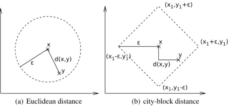
Figure2.1illustrates the definition of a neighborhood in a 2-dimensional contin-uous search spaceR2for Euclidean distances (Fig.2.1(a)) and Manhattan distances (Fig.2.1(b)). Using an open ball, all solutions y where d(x,y)<εare neighboring solutions to x. For Euclidean distances, we use d(x,y):=(x1−y1)2+ (x2−y2)2 and neighboring solutions are all solutions that can be found inside of a circle around x with radius ε. For city-block distances, we use d(x,y):=|x1−y1|+|x2−y2| and all solutions inside a rhombus with the vertices (x1−ε,y1),(x1,y1+ε),(x1+
ε,y1),(x1,y1−ε) are neighboring solutions.
It is problematic to apply metric search spaces to problems where no meaningful similarities between different decision alternatives can be defined or do not exist. For such problems, the only option is to define a trivial topology (see p.16) which assumes that all solutions are neighbors and no meaningful structure on the search
Fig. 2.1 Neighborhoods on a 2-dimensional Euclidean space using different metrics
space exists. However, practitioners (as well as users) are used to metric search spaces and often seek to apply them also to problems where no meaningful similar-ities between different decision alternatives can be defined. This is a mistake as a metric search space does not model such a problem in an appropriate way.
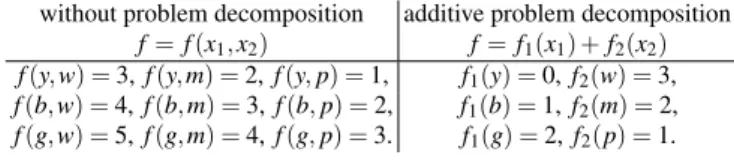
We want to give an example. We assume a search space containing four differ-ent fruits (apple (a), banana (b), pear (p), and orange (o)). This search space forms a trivial topology({a,b,p,o},{/0,{a,b,p,o}}as no meaningful distances between the four fruits exist and all solutions are neighbors of each other. Nevertheless, we can define a metric search space X={0,1}2 for the problem. Each solution ((0,0),(0,1),(1,0), and(1,1)) represents one fruit. Although the original problem defines no similarities, the use of a metric space induces that the solution (0,0) is more similar to(0,1)than to(1,1)(using Hamming distance (2.7)). Therefore, a metric space is inappropriate for the problem definition as it defines similarities where no similarities exist. A more appropriate model would be x∈ {0, . . . ,3}and using Hamming distance (2.8). Then, all distances between the different solutions are equal and all solutions are neighbors.
A different problem can occur if the metric used is not appropriate for the prob-lem and existing “similarities” between different decision alternatives do not fit the similarities between different solutions described by the model. The metric defined for the problem model is a result of the choice of the decision variables. Any choice of decision variables{x1, . . . ,xn}allows the definition of a metric space and, thus, defines similarities between different solutions. However, if the metric induced by the use of the decision variables does not fit the metric of the problem description, the problem model is inappropriate.
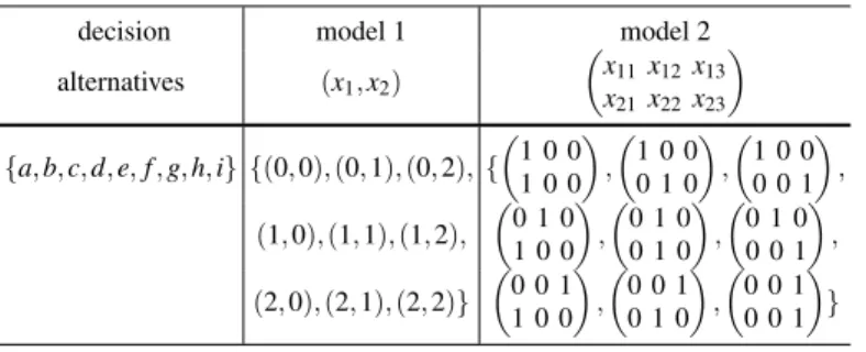
Table2.1illustrates this situation. We assume that there are s=9 different de-cision alternatives{a,b,c,d,e,f,g,h,i}. We assume that the decision alternatives form a metric space (using the Hamming metric (2.8)), where the distances be-tween all elements are equal. Therefore, all decision alternatives are neighbors (for ε>1). In the first problem model (model 1), we use a metric space X ={0,1,2}2 and Hamming metric (2.8). Therefore, each decision alternative is represented by
(x1,x2)with xi∈ {0,1,2}. For the Hamming metric, each solution has four neigh-bors. For example, decision alternative(1,1)is a neighbor of(1,2)but not of(2,2). Model 1 results in a different neighborhood in comparison to the original decision alternatives. Model 2 is an example of a different metric space. In this model, we use binary variables xi jand the search space is defined as X=xi j, where xi j∈ {0,1}. We have an additional restriction,∑jxi j=1, where i∈ {1,2}and j∈ {1,2,3}. Again, Hamming distance (2.8) can be used. Forε=1.1, no neighboring solutions exist. Forε=2.1, each solution has four neighbors. We see that different models for the same problem result in different neighborhoods which do not necessarily coincide with the neighborhoods of the original problem.
Table 2.1 Two different search spaces for a problem
decision model 1 model 2
alternatives (x1,x2) x11x12x13 x21x22x23 {a,b,c,d,e,f,g,h,i} {(0,0),(0,1),(0,2),{ 1 0 0 1 0 0 , 1 0 0 0 1 0 , 1 0 0 0 0 1 , (1,0),(1,1),(1,2), 0 1 0 1 0 0 , 0 1 0 0 1 0 , 0 1 0 0 0 1 , (2,0),(2,1),(2,2)} 0 0 1 1 0 0 , 0 0 1 0 1 0 , 0 0 1 0 0 1 }
The examples illustrate that selecting an appropriate model is important. For the same problem, different models are possible which can result in different neighbor-hoods. We must select the model such that the metric induced by the model fits well the metric that exists for the decision alternatives. Although, in the problem descrip-tion no neighborhood needs to be defined, usually a nodescrip-tion of neighborhoods exist. Users that formulate a model description often know which decision alternatives are similar to each other as they have a feeling about which decision alternatives result in the same outcome. When constructing the model, we must ensure that the neighborhood induced by the model fits well the (often intuitive) neighborhood for-mulated by the user.
Relevant aspects which determine the resulting neighborhood of a model are the type and number of decision variables. The types of decision variables should be determined by the properties of the decision alternatives. If decision alternatives are continuous (for example, choosing the right amount of crushed ice for a drink), the use of continuous decision variables in the model is useful and discrete deci-sion variables should not be used. Analogously, for discrete decideci-sion alternatives, discrete decision variables and combinatorial models should be preferred. For ex-ample, the number of ice cubes in a drink should be modelled using integers and not continuous variables.
The number of decision variables used in the model also affects the resulting neighborhood. For discrete models, there are two extremes: first, we can model s different decision alternatives by using only one decision variable that can take s
different values. Second, we can use l=log2(s)binary decision variables xi∈ {0,1} (i∈ {1, . . . ,l}). If we use Hamming distance (2.8) and define neighboring solutions as d(x,y)≤1, then all possible solutions are neighbors if we use only one decision variable. In contrast, each solution x∈ {0,1}lhas only l neighbors y∈ {0,1}l, where d(x,y)≤1. We see that using different numbers of decision variables for modeling the decision alternatives results in completely different neighborhoods. In general, a high-quality model is a model where the neighborhoods defined in the model fit well the neighborhoods that exist in the problem.
2.3.3 Fitness Landscapes
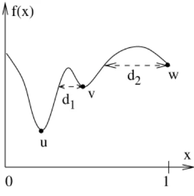
For combinatorial search spaces where a metric is defined, we can introduce the con-cept of fitness landscape (Wright, 1932). A fitness landscape(X,f,d)of a problem instance consists of a set of solutions x∈X , an objective function f that measures the quality of each solution, and a distance measure d. Figure2.2is an example of a one-dimensional fitness landscape.
We denote dmin=minx,y∈X(d(x,y)), where x=y, as the minimum distance be-tween any two elements x and y of a search space. Two solutions x and y are de-noted as neighbors if d(x,y) =dmin. Often, d can be normalized to dmin=1. A fitness landscape can be described using a graph GLwith a vertex set V =X and an edge set E={(x,y)∈X×X|d(x,y) =dmin}(Reeves, 1999a; Merz and Freisleben, 2000b). The objective function assigns an objective value to each vertex. We as-sume that each solution has at least one neighbor and the resulting graph is con-nected. Therefore, an edge exists between neighboring solutions. The distance be-tween two solutions x,y∈X is proportional to the number of nodes that are on the path of minimal length between x and y in the graph GL. The maximum distance dmax=maxx,y∈X(d(x,y))between any two solutions x,y∈X is called the diameter diam GLof the landscape.
We want to give an example: We use the search space defined by model 1 in Table2.1and Hamming distance (2.8). Then, all solutions where only one decision variable is different are neighboring solutions (d(x,y) =dmin). The maximum dis-tance dmax=2. More details on fitness landscapes can be found in Reeves and Rowe (2003, Chap. 9) or Deb et al (1997).
2.3.4 Optimal Solutions
A globally optimal solution for an optimization problem is defined as the solution x∗∈X , where f(x∗)≤f(x)for all x∈X (minimization problem). For the definition of a globally optimal solution, it is not necessary to define the structure of the search space, a metric, or a neighborhood.
Given a problem instance(X,f)and a neighborhood function N, a feasible so-lution x∈X is called locally optimal (minimization problem) with respect to N if
f(x)≤f(x) for all x∈N(x). (2.10) Therefore, locally optimal solutions do not exist if no neighborhood is defined. Fur-thermore, the existence of local optima is determined by the neighborhood definition used as different neighborhoods can result in different locally optimal solutions.
Fig. 2.2 Locally and globally
optimal solutions
Figure2.2illustrates the differences between locally and globally optimal so-lutions and shows how local optima depend on the definition of N. We have a one-dimensional minimization problem with x∈[0,1]∈R. We assume an objec-tive function f that assigns objecobjec-tive values to all x∈X . Independently of the neighborhood used, u is always the globally optimal solution. If we use the 1-dimensional Euclidean distance (2.6) as metric and define a neighborhood around x as N(x) ={y|y∈X and d(x,y)≤ε}the solution v is a locally optimal solution if ε<d1. Analogously, w is locally optimal for all neighborhoods withε<d2. For
ε≥d2, the only locally optimal solution is the globally optimal solution u.
The modality of a problem describes the number of local optima in the prob-lem. Unimodal problems have only one local optimum (which is also the global optimum) whereas multi-modal problems have multiple local optima. In general, multi-modal problems are more difficult for guided search methods to solve than unimodal problems.
2.4 Properties of Optimization Problems
The purpose of optimization algorithms is to find high-quality solutions for a prob-lem. If possible, they should identify either optimal solutions x∗, near-optimal solu-tions x∈X , where f(x)−f(x∗)is small, or at least locally optimal solutions.
Problem difficulty describes how difficult it is to find an optimal solution for a specific problem or problem instance. Problem difficulty is defined independently
of the optimization method used. Determining the difficulty of a problem is often a difficult task as we have to prove that that there are no optimization methods that can better solve the problem. Statements about the difficulty of a problem are method-independent as they must hold for all possible optimization methods.
We know that different types of optimization methods lead to different search performance. Often, optimization methods perform better if they exploit some char-acteristics of an optimization problem. In contrast, methods that do not exploit any problem characteristics, like black-box optimization techniques, usually show low performance. For an example, we have a look at random search. In random search, solutions x∈X are iteratively chosen in a random order. We want to assume that each solution is considered only once by random search. When random search is stopped, it returns the best solution found. During random search, new solutions are chosen randomly and no problem-specific information about the structure of the problem or previous search steps is used. The number of evaluations needed by ran-dom search is the number of elements drawn from X , which is independent of the problem itself (if we assume a unique optimal solution). Consequently, a distinction between “easy” and “difficult” problems is meaningless when random search is the only available optimization method.
The following sections study properties of optimization problems. Section2.4.1 starts with complexity classes which allow us to formulate bounds on the perfor-mance of algorithmic methods. This allows us to make statements about the dif-ficulty of a problem. Then, we continue with properties of optimization problems that can be exploited by modern heuristics. Section 2.4.2introduces the locality of a problem and presents corresponding measurements. The locality of a problem is exploited by guided search methods which perform well if problem locality is high. Important for high locality is a proper definition of a metric on the search space. Finally, Sect. 2.4.3 discusses the decomposability of a problem and how recombination-based optimization methods exploit a problem’s decomposability.
2.4.1 Problem Difficulty
The complexity of an algorithm is the effort (usually time or memory) that is nec-essary to solve a particular problem. The effort depends on the input size, which is equal to the size n of the problem to be solved. The difficulty or complexity of a problem is the lowest possible effort that is necessary to solve the problem.
Therefore, problem difficulty is closely related to the complexity of algorithms. Based on the complexity of algorithms, we are able to find upper and lower bounds on the problem difficulty. If we know that an algorithm can solve a problem, we automatically have an upper bound on the difficulty of the problem, which is just the complexity of the algorithm. For example, we study the problem of finding a friend’s telephone number in the telephone book. The most straightforward approach is to search through the whole book starting from “A”. The effort for doing this increases linearly with the number of names in the book. Therefore, we have an upper bound
on the difficulty of the problem (problem has at most linear complexity) as we know a linear algorithm that can solve the problem. A more effective way to solve this problem is bisection or binary search which iteratively splits the entries of the book into halves. With n entries, we only need log(n)search steps to find the number. So, we have a new, improved, upper bound on problem difficulty.
Finding lower bounds on the problem difficulty is more difficult as we have to show that no algorithm exists that needs less effort to solve the problem. Our prob-lem of finding a friend’s name in a telephone book is equivalent to the probprob-lem of searching an ordered list. Binary search which searches by iteratively splitting the list into halves is optimal and there is no method with lower effort (Knuth, 1998). Therefore, we have a lower bound and there is no algorithm that needs less than log(n)steps to find an address in a phone book with n entries. A problem is called closed if the upper and lower bounds on its problem difficulty are identical. Conse-quently, the problem of searching an ordered list is closed.
This section illustrates how bounds on the difficulty of problems can be derived by studying the effort of optimization algorithms that are used to solve the problems. As a result, we are able to classify problems as easy or difficult with respect to the performance of the best-performing algorithm that can solve the problem.
The following paragraphs give an overview of the Landau notation which is an instrument for formulating upper and lower bounds on the effort of optimization algorithms. Thus, we can also use it for describing problem difficulty. Then, we illustrate that each optimization problem can also be modeled as a decision problem of the same difficulty. Finally, we illustrate different complexity classes (P, NP, NP-hard, and NP-complete) and discuss the tractability of decision and optimization problems.
2.4.1.1 Landau Notation
The Landau notation (which was introduced by Bachmann (1894) and made popular by the work of Landau (1974)) can be used to compare the asymptotic growth of functions and is helpful when measuring the complexity of problems or algorithms. It allows us to formulate asymptotic upper and lower bounds on function values. For example, Landau notation can be used to determine the minimal amount of memory or time that is necessary to solve a specific problem. With n∈N, c∈R, and f,g :N→Rthe following bounds can be described using the Landau symbols: • asymptotic upper bound (“big O notation”):
f ∈O(g)⇔ ∃c>0∃n0>0∀n≥n0:|f(n)| ≤c|g(n)|: f is dominated by g. • asymptotically negligible (“little o notation”):
f ∈o(g)⇔ ∀c>0∃n0>0∀n≥n0:|f(n)|<c|g(n)|: f grows slower than g. • asymptotic lower bound:
f ∈Ω(g)⇔g∈O(f): f grows at least as fast as g. • asymptotically dominant:
• asymptotically tight bound:
f ∈Θ(g)⇔g∈O(f)∧f ∈O(g): g and f grow at the same rate.
Using this notation, it is easy to compare the difficulty of different problems: using O(g)andΩ(g), it is possible to give an upper, respectively lower bound for the asymptotic running time f of algorithms that are used to solve a problem. It is im-portant to have in mind that lower bounds on problem difficulty hold for all possible optimization problems for a specific problem. In contrast, upper bounds only indi-cate that there is at least one algorithm that can solve the problem with this effort but there are also other algorithms where a higher effort is necessary. The Landau nota-tion does not consider constant factors since these mainly depend on the computer or implementation used to solve the problem. Therefore, constants do not directly influence the difficulty of a problem.
We give three small examples. In problem 1, we want to find the smallest num-ber in an unordered list of n numnum-bers. The complexity of this problem is O(n)(it increases linearly with n) when using linear search and examining all possible ele-ments in the list. As it is not possible to solve this problem faster than linear, there is no gap between the lower boundΩ(n)and upper bound O(n). In problem 2, we want to find an element in an ordered list with n items (for example finding a tele-phone number in the teletele-phone book). Binary search (bisection) iteratively splits the list into two halves and can find any item in log(n)search steps. Therefore, the upper bound on the complexity of this problem is O(log(n)). Again, the lower bound is equal to the upper bound (Harel and Rosner, 1992; Cormen et al, 2001) and the complexity of the problem isΘ(log(n)). Finally, in problem 3 we want to sort an ar-ray of n arbitrary elements. Using standard sorting algorithms like merge sort (Cor-men et al, 2001) it can be solved in O(n log(n)). As the lower bound isΩ(n log(n)), the difficulty of this problem isΘ(n log(n)).
2.4.1.2 Optimization Problems, Evaluation Problems, and Decision Problems
To derive upper and lower bounds on problem difficulty, we need a formal descrip-tion of the problem. Thus, at least the soludescrip-tions x∈X and the objective function f : X→Rmust be defined. The search space can be very trivial (e.g. have a trivial topology) as the definition of a neighborhood structure is not necessary. Developing bounds is difficult for problems where the objective function does not systematically assign objective values to each solution. Although describing X and f is sufficient for formulating a problem model, in most problems of practical relevance the size |X| of the search space is large and, thus, the direct assignment of objective val-ues to each possible solution is often very time-consuming and not appropriate for building an optimization model that should be solved by a computer.
To overcome this problem, we can define each optimization problem implicitly using two algorithmsAX andAf, and two sets of parameters SX and Sf. Given a set of parameters SX, the algorithmAX(x,SX)decides whether the solution x is an element of X , i.e. whether x is a feasible solution. Given a set of parameters Sf, the algorithmAf(x,Sf)calculates the objective value of a solution x. Therefore,
Af(x,Sf)is equivalent to the objective function f(x). For givenAX andAf, we can define different instances of a combinatorial optimization problem by assigning different values to the parameters in SXand Sf.
We want to give an example. We have a set of s different items and want to find a subset of n items with minimal weight. Then, the algorithmAXchecks whether a solution x is feasible. The set SXcontains only one parameter which is the number n of items that should be found. If x contains exactly n items,AX(x,SX)indicates that x is a feasible solution. The parameters Sf are the weights wiof the different items. AlgorithmAf calculates the objective value of a feasible solution x by summing up the weights of the n items ( f(x,w) =∑wi) using the solution x and the weights wi. Using these definitions, we can formulate an optimization problem as:
Given are the two algorithmsAXandAfand representations of the parameters SXand Sf.
The goal is to find the optimal feasible solution.
This formulation of an optimization problem is equivalent to (2.3) (p.15). The al-gorithmAX checks whether all constraints are met andAf calculates the objective value of x. Analogously, the evaluation version of an optimization problem can be defined as:
Given are the two algorithmsAXandAfand representations of the parameters SXand Sf.
The goal is to find the objective value of the optimal solution.
Finally, the decision version (also known as recognition version) of an optimization problem can be defined as:
Given are the algorithmsAXandAf, representations of the parameters SXand Sf, and an
integer L. The goal is to decide whether there is a feasible solution x∈X such that f(x)≤L. The first two versions are problems where an optimal solution has to be found, whereas in the decision version of an optimization problem a question has to be answered either by yes or no. We denote feasible solutions x whose objective value f(x)≤L as yes-solutions. We can solve the decision version of the optimization problem by solving the original optimization problem, calculating the objective value f(x∗)of the optimal solution x∗, and deciding whether f(x∗)is greater than L. Therefore, the difficulty of the three versions is roughly the same if we assume that f(x∗), respectivelyAf(x∗,Xf), is easy to compute (Papadimitriou and Steiglitz, 1982, Chap. 15.2). If this is the case, all three versions are equivalent.
We may ask why we want to formulate an optimization as a decision problem which is much less intuitive? The reason is that in computational complexity the-ory, many statements on problem difficulty are formulated for decision (and not optimization) problems. By formulating optimization problems as decision prob-lems, we can apply all these results to optimization problems. Therefore, complexity classes which can be used to categorize decision problems in classes with different difficulty (compare the following paragraphs) can also be used for categorizing opti-mization problems. For more information on the differences between optiopti-mization, evaluation, and decision versions of an optimization problem, we refer the interested reader to Papadimitriou and Steiglitz (1982, Chap. 15) or Harel and Rosner (1992).
2.4.1.3 Complexity Classes
Computational complexity theory ((Hartmanis and Stearns, 1965; Cook, 1971; Garey and Johnson, 1979; Papadimitriou and Yannakakis, 1991; Papadimitriou, 1994; Arora and Barak, 2009) allows us to categorize decision problems in different groups based on their difficulty. The difficulty of a problem is defined with respect to the amount of computational resources that are at least necessary to solve the problem.
In general, the effort (amount of computational resources) that is necessary to solve an optimization problem of size n is determined by its time and space com-plexity. Time complexity describes how many iterations or number of search steps are necessary to solve a problem. Problems are more difficult if more time is nec-essary. Space complexity describes the amount of space (usually memory on a com-puter) that is necessary to solve a problem. As for time, problem difficulty increases with higher space complexity. Usually, time and space complexity depend on the input size n and we can use the Landau notation to describe upper and lower bounds on them. A complexity class is a set of computational problems where the amount of computational resources that are necessary to solve the problem shows the same asymptotic behavior. For all problems that are contained in one complexity class, we can give bounds on the computational complexity (in general, time and space complexity). Usually, the bounds depend on the size n of the problem, which is also called its input size. Usually, n is much smaller than the size|X|of the search space. Typical bounds are asymptotic lower or upper bounds on the time that is necessary to solve a particular problem.
Complexity Class P
The complexity class P (P stands for polynomial) is defined as the set of decision problems that can be solved by an algorithm with worst-case polynomial time com-plexity. The time that is necessary to solve a decision problem in P is asymptotically bounded (for n>n0) by a polynomial function O(nk). For all problems in P, an algorithm exists that can solve any instance of the problem in time that is O(nk), for some k. Therefore, all problems in P can be solved effectively in the worst case. As we showed in the previous section that all optimization problems can be formulated as decision problems, the class P can be used to categorize optimization problems.
Complexity Class NP
The class NP (which stands for non-deterministic polynomial time) describes the set of decision problems where a yes solution of a problem can be verified in polynomial time. Therefore, both the formal representation of a solution x and the time it takes to check its validity (to check whether it is a yes solution) must be polynomial or polynomially-bounded.
Therefore, all problems in NP have the property that their yes solutions can be checked effectively. The definition of NP says nothing about the time necessary for verifying no solutions and a problem in NP can not necessarily be solved in polynomial time. Informally, the class NP consists of all “reasonable” problems of practical importance where a yes solution can be verified in polynomial time: this means the objective value of the optimal solution can be calculated fast. For problems not in NP, even verifying that a solution is valid (is a yes answer) can be extremely difficult (needs exponential time).
An alternative definition of NP is based on the notion of non-deterministic al-gorithms. Non-deterministic algorithms are algorithms which have the additional ability to guess any verifiable intermediate result in a single step. If we assume that we find a yes solution for a decision problem by iteratively assigning values to the decision variables, a non-deterministic algorithm always selects the value (possibil-ity) that leads to a yes answer, if a yes answer exists for the problem. Therefore, we can view a non-deterministic algorithm as an algorithm that always guesses the right possibility whenever the correctness can be checked in polynomial time. The class NP is the set of all decision problems that can be solved by a non-deterministic algorithm in worst-case polynomial time. The two definitions of NP are equivalent to each other. Although non-deterministic algorithms cannot be executed directly by conventional computers, this concept is important and helpful for the analysis of the computational complexity of problems.
All problems that are in P also belong to the class NP. Therefore, P⊆NP. An important question in computational complexity is whether P is a proper subset of NP (P⊂NP) or whether NP is equal to P (P=NP). So far, this question is not finally answered (Fortnow, 2009) but most researchers assume that P=NP and there are problems that are in NP, but not in P.
In addition to the classes P and NP, there are also problems where yes solutions cannot be verified in polynomial time. Such problems are very difficult to solve and are, so far, of only little practical relevance.
Tractable and Intractable Problems
When solving an optimization problem, we are interested in the running time of the algorithm that is able to solve the problem. In general, we can distinguish between polynomial running time and exponential running time. Problems that can be solved using a polynomial-time algorithm (there is an upper bound O(nk)on the running time of the algorithm, where k is constant) are tractable. Usually, tractable problems are easy to solve as running time increases relatively slowly with larger input size n. For example, finding the lowest element in an unordered list of size n is tractable as there are algorithms with time complexity that is O(n). Spending twice as much effort solving the problem allows us to solve problems twice as large.
In contrast, problems are intractable if they cannot be solved by a polynomial-time algorithm and there is a lower bound on the running polynomial-time which isΩ(kn), where k>1 is a constant and n is the problem size (input size). For example, guessing the
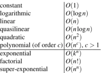
correct number for a digital door lock with n digits is an intractable problem, as the time necessary for finding the correct key isΩ(10n). Using a lock with one more digit increases the number of required search steps by a factor of 10. For this problem, the size of the problem is n, whereas the size of the search space is |X|=10n. The effort to find the correct key depends on n and increases at the same rate as the size of the search space. Table2.2lists the growth rate of some common functions ordered by how fast they grow.
Table 2.2 Polynomial (top)
and exponential (bottom) functions
constant O(1)
logarithmic O(log n)
linear O(n)
quasilinear O(n log n)
quadratic O(n2)
polynomial (of order c) O(nc), c>1
exponential O(kn)
factorial O(n!)
super-exponential O(nn)
We can identify three different types of problems with different difficulty. • Tractable problems with known polynomial-time algorithms. These are easy
problems. All tractable problems are in P.
• Provably intractable problems, where we know that there is no polynomial-time algorithm. These are difficult problems.
• Problems where no polynomial-time algorithm is known but intractability has not yet been shown. These problems are also difficult.
NP-Hard and NP-Complete
All decision problems that are in P are tractable and thus can be easily solved using the “right” algorithm. If we assume that P=NP, then there are also problems that are in NP but not in P. These problems are difficult as no polynomial-time algorithms exist for them.
Among the decision problems in NP, there are problems where no polynomial algorithm is available and which can be transformed into each other with polyno-mial effort. Consequently, a problem is denoted NP-hard if an algorithm for solving this problem is polynomial-time reducible to an algorithm that is able to solve any problem in NP. A problem A is polynomial-time reducible to a different problem B if and only if there is a transformation that transforms any arbitrary solution x of A into a solution xof B in polynomial time such that x is a yes instance for A if and only if xis a yes instance for B. Informally, a problem A is reducible to some other problem B if problem B either has the same difficulty or is harder than problem A. Therefore, NP-hard problems are at least as hard as any other problem in NP, al-though they might be harder. Therefore, NP-hard problems are not necessarily in NP.
Cook (1971) introduced the set of NP-complete problems as a subset of NP. A decision problem A is denoted NP-complete if
• A is in NP and • A is NP-hard.
Therefore, no other problem in NP is more than a polynomial factor harder than any NP-complete problem. Informally, NP-complete problems are the most difficult problems that are in NP.
All NP-complete problems form one set as all NP-complete problems have the same complexity. However, it is as yet unclear whether NP-complete problems are tractable. If we are able to find a polynomial-time algorithm for any one of the NP-complete problems, then every NP-NP-complete problem can be solved in polynomial time. Then, all other problems in NP can also be solved in polynomial time (are tractable) and thus P=NP. On the other hand, if it can be shown that one NP-complete problem is intractable, then all NP-NP-complete problems are intractable and P=NP.
Summarizing our discussion, we can categorize optimization problems with re-spect to the computational effort that is necessary for solving them. Problems that are in P are usually easy as algorithms are known that solve such problems in pol-ynomial time. Problems that are NP-complete are difficult as no polpol-ynomial-time algorithms are known. Decision problems that are not in NP are even more difficult as we could not evaluate in polynomial time whether a particular solution for such a problem is feasible. To be able to calculate upper and lower bounds on problem complexity, usually well-defined problems are necessary that can be formulated in functional form.
2.4.2 Locality
In general, the locality of a problem describes how well the distances d(x,y) be-tween any two solutions x,y∈X correspond to the difference of the objective values |f(x)−f(y)|(Lohmann, 1993; Rechenberg, 1994; Rothlauf, 2006). The locality of a problem is high if neighboring solutions have similar objective values. In contrast, the locality of a problem is low if low distances do not correspond to low differences of the objective values. Relevant determinants for the locality of a problem are the metric defined on the search space and the objective function f .
In the heuristic literature, there are a number of studies on locality for discrete de-cision variables (Weicker and Weicker, 1998; Rothlauf and Goldberg, 1999, 2000; Gottlieb and Raidl, 2000; Gottlieb et al, 2001; Whitley and Rowe, 2005; Caminiti and Petreschi, 2005; Raidl and Gottlieb, 2005; Paulden and Smith, 2006) as well as for continuous decision variables (Rechenberg, 1994; Igel, 1998; Sendhoff et al, 1997b,a). For continuous decision variables, locality is also known as causality. High and low locality correspond to strong and weak causality, respectively. Al-though causality and locality describe the same concept and causality is the older
one, we refer to the concept as locality as it is currently more often used in the literature.
Guided search methods are optimization approaches that iteratively sample solu-tions and use the objective values of previously sampled solusolu-tions to guide the future search process. In contrast to random search which samples solutions randomly and uses no information about previously sampled solutions, guided search methods dif-ferentiate between promising (for maximization problems these are solutions with high objective values) and non-promising (solutions with low objective values) areas in the fitness landscape. New solutions are usually generated in the neighborhood of promising solutions with high objective values. A prominent example of guided search is greedy search (see Sect. 3.4.1).
The locality of optimization problems has a strong impact on the performance of guided search methods. Problems with high locality allow guided search methods to find high-quality solutions in the neighborhood of already found good solutions. Furthermore, the underlying idea of guided search methods to move in the search space from low-quality solutions to high-quality solutions works well if the problem has high locality. In contrast, if a problem has low locality, guided search methods cannot make use of previous search steps to extract information that can be used for guiding the search. Then, for problems with low locality, guided search methods behave like random search.
One of the first approaches to the question of what makes problems difficult for guided search methods, was the study of deceptive problems by Goldberg (1987) which was based on the work of Bethke (1981). In deceptive problems, the objec-tive values are assigned in such a way to the solutions that guided search methods are led away from the global optimal solution. Therefore, based on the structure of the fitness landscape (Weinberger, 1990; Manderick et al, 1991; Deb et al, 1997), the correlation between the fitness of solutions can be used to describe how difficult a specific problem is to solve for guided search methods. For an overview of correla-tion measurements and problem difficulty we refer to B¨ack et al (1997, Chap. B2.7) or Reeves and Rowe (2003).
The following paragraphs present approaches that try to determine what makes a problem difficult for guided search. Their general idea is to measure how well the metric defined on the search space fits the structure of the objective function. A high fit between metric and structure of the fitness function makes a problem easy for guided search methods.
2.4.2.1 Fitness-Distance Correlation
A straightforward approach for measuring the difficulty of problems for guided search methods has been presented in Jones and Forrest (1995). They assumed that the difficulty of an optimization problem is determined by how the objective values are assigned to the solutions x∈X and what metric is defined on X . Combining both aspects, problem difficulty can be measured by the fitness-distance correlation coefficient