Imputation Techniques for Non-ordered
Categorical Missing Data
by
Innocent Karangwa
A thesis submitted in fulfilment for the
degree of Doctor of Philosophy in Statistics
at the
Faculty of Natural Sciences
Department of Statistics and Population Studies
Supervisor: Prof. Danelle Kotze Co-Supervisor: Prof. Renette Blignaut
February 2016
Declaration of authorship
I declare that Imputation Techniques for Non-ordered Categorical Missing Data is my own work, that it has not been submitted for any degree or examination in any other university and that all the sources I used or quoted have been indicated and acknowledged by appropriate references.
Innocent Karangwa Signed: Date: i
Missing data
Missing at random
Multiple imputation
Multivariate normal imputation
Multiple imputation by chained equations
Categorical data ii
Abstract
Missing data are common in survey data sets. Enrolled subjects do not often have data recorded for all variables of interest. The inappropriate handling of missing data may lead to bias in the estimates and incorrect inferences. Therefore, spe-cial attention is needed when analysing incomplete data. The multivariate normal imputation (MVNI) and the multiple imputation by chained equations (MICE) have emerged as the best techniques to impute or fill in missing data. The former assumes a normal distribution of the variables in the imputation model, but can also handle missing data whose distributions are not normal. The latter fills in missing values taking into account the distributional form of the variables to be imputed. The aim of this study was to determine the performance of these meth-ods when data are missing at random (MAR) or completely at random (MCAR) on unordered or nominal categorical variables treated as predictors or response variables in the regression models. Both dichotomous and polytomous variables were considered in the analysis. The baseline data used was the 2007 Demographic and Health Survey (DHS) from the Democratic Republic of Congo. The analysis model of interest was the logistic regression model of the woman’s contraceptive method use status on her marital status, controlling or not for other covariates (continuous, nominal and ordinal). Based on the data set with missing values, data sets with missing at random and missing completely at random observations on either the covariates or response variables measured on nominal scale were first simulated, and then used for imputation purposes. Under MVNI method, un-ordered categorical variables were first dichotomised, and then K−1 (where K is the number of levels of the categorical variable of interest) dichotomised variables were included in the imputation model, leaving the other category as a reference. These variables were imputed as continuous variables using a linear regression model. Imputation with MICE considered the distributional form of each variable to be imputed. That is, imputations were drawn using binary and multinomial logistic regressions for dichotomous and polytomous variables respectively. The performance of these methods was evaluated in terms of bias and standard errors in regression coefficients that were estimated to determine the association between
iii
the woman’s contraceptive methods use status and her marital status, controlling or not for other types of variables. The analysis was done assuming that the sam-ple was not weighted first, then the samsam-ple weight was taken into account to assess whether the sample design would affect the performance of the multiple imputation methods of interest, namely MVNI and MICE. As expected, the results showed that for all the models, MVNI and MICE produced less biased smaller standard errors than the case deletion (CD) method, which discards items with missing values from the analysis. Moreover, it was found that when data were missing (MCAR or MAR) on the nominal variables that were treated as predictors in the regression model, MVNI reduced bias in the regression coefficients and standard errors compared to MICE, for both unweighted and weighted data sets. On the other hand, the results indicated that MICE outperforms MVNI when data were missing on the response variables, either the binary or polytomous. Furthermore, it was noted that the sample design (sample weights), the rates of missingness and the missing data mechanisms (MCAR or MAR) did not affect the behaviour of the multiple imputation methods that were considered in this study. Thus, based on these results, it can be concluded that when missing values are present on the outcome variables measured on a nominal scale in regression models, the distribu-tional form of the variable with missing values should be taken into account. When these variables are used as predictors (with missing observations), the parametric imputation approach (MVNI) would be a better option than MICE.
Acknowledgements
Writing this thesis has been an extremely good experience full of challenges and drawbacks I could not have navigated through alone. Fortunately, I was blessed to have many wonderful people around me whose support, insight, and knowledge of statistics have made this journey so easy.
First and foremost, I owe this dissertation to my supervisors, Professor Danelle Kotze and Professor Renette Blignaut who were always there for me when I needed them most. Their patient support was the strongest inspiration to per-severe in the face of various obstacles. They were not only helpful in giving me advice in both composition and content, but also in providing me with financial support.
I would like to thank the entire Department of Statistics and Population Studies at the University of the Western Cape for providing an incredibly stimu-lating learning environment and statistical knowledge.
My friends and colleagues at this university were so dear to me, having been there through trying times. I would like to recognise their valuable opinions and experience. In particular, I would like to acknowledge Dr Siaka Lougue, Mr Aris-tide Bado, Mr Yasser Bucyana, Mr Justin Rutikanga and Mr Adam Andani for their extremely valuable conversations, feedback and any other kind of contribu-tion to my thesis. I wish them all the future success they deserve.
Special thanks and recognition are also owed to the DST-NRF Centre of Excellence in Mathematical and Statistical Sciences (CoE-MaSS) that funded this research during the final year of my studies.
Finally, I also thank everyone who gave me emotional support.
v
Contents
Declaration of authorship i Keywords ii Abstract iii Acknowledgements v List of figures xList of tables xxii
1 Introduction 1
1.1 Background on missing data . . . 1
1.1.1 Sampling and nonresponse . . . 1
1.1.2 Missing data. . . 3
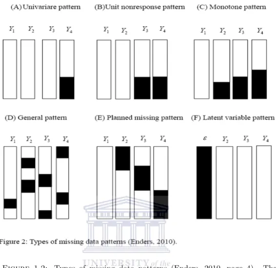
1.1.3 Missing data patterns. . . 5
1.1.4 Missingness mechanisms . . . 6
1.1.5 Testing for missingness mechanisms . . . 9
1.2 Motivation for the study . . . 11
1.3 Significance of the study . . . 14
1.4 Research objectives . . . 14
1.5 Research questions . . . 15
1.6 Hypotheses . . . 16
1.7 Research Design. . . 16
1.8 Thesis overview . . . 16
2 Markov Chain Monte Carlo process 19 2.1 Introduction . . . 19
2.2 Monte Carlo integration . . . 20
2.3 Importance sampling . . . 23 vi
Contents vii
2.4 Markov Chain Monte Carlo . . . 26
2.4.1 Introduction . . . 26
2.4.2 Metropolis-Hastings algorithm . . . 28
2.4.3 Gibbs sampling . . . 30
2.5 Markov Chain Monte Carlo methods in the presence of missing data 35 2.5.1 Introduction . . . 35
2.5.2 Markov Chain Monte Carlo versus missing data . . . 35
2.6 Summary of the chapter . . . 36
3 Literature review on missing data methods 38 3.1 Introduction . . . 38
3.2 Single-based imputation methods . . . 39
3.2.1 Mean imputation . . . 39
3.2.2 Hot-deck imputation . . . 39
3.2.3 Cold-deck imputation. . . 40
3.2.4 Regression imputation . . . 40
3.2.5 Imputation using interpolation. . . 41
3.3 Model-based methods . . . 41
3.3.1 Expectation maximisation . . . 41
3.3.2 Maximum likelihood method . . . 42
3.4 Multiple imputation-based methods . . . 43
3.4.1 Introduction . . . 43
3.4.2 Description of multivariate normal imputation . . . 45
3.4.3 Description of multiple imputation by chained equations . . 48
3.4.4 Multivariate normal imputation versus multiple imputation by chained equation: a practical example using a survey data set to impute missing values of continuous variables . . 52
3.4.4.1 Introduction . . . 52
3.4.4.2 Data . . . 52
3.4.4.3 Analysis method . . . 54
3.4.4.4 Findings . . . 54
3.4.4.5 Conclusion . . . 59
3.4.5 Multivariate normal imputation versus multiple imputation by chained equations of categorical data . . . 59
3.5 Summary of the chapter . . . 62
4 Methodology 63 4.1 Description of data set and variables used in the study . . . 63
4.2 Simulation of the data sets with missing values. . . 65
4.3 Missing data models . . . 65
4.4 Analysis method . . . 68
4.4.1 Imputation of missing values . . . 68
4.4.2 Model development and computation of the performance measures . . . 73
4.4.3 Imputation models’ diagnostics . . . 73
4.5 Summary of the chapter . . . 74
5 Results 76 5.1 Introduction . . . 76
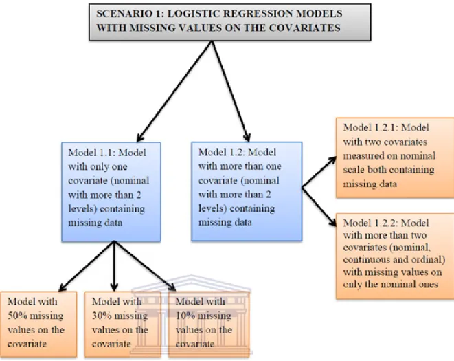
5.2 Scenario 1: Logistic regression models with missing values on the covariates . . . 77
5.2.1 Model 1.1: Binary logistic regression model with missing values on a single covariate measured on a nominal scale . . 78
5.2.1.1 Results when 50% of data are missing at random or completely at random on the covariate . . . 78
Descriptive statistics . . . 78
Performance measures . . . 83
Model diagnostics . . . 86
5.2.1.2 Results when 30% of data are missing at random or completely at random on the covariate . . . 87
Descriptive statistics . . . 87
Performance measures . . . 90
Model diagnostics . . . 93
5.2.1.3 Results when 10% of data are missing at random or completely at random on the covariate . . . 94
Descriptive statistics . . . 94
Performance measures . . . 97
Model diagnostics . . . 100
5.2.2 Model 1.2: Binary logistic regression model with more than two covariates in which two are measured on a nominal scale containing missing values . . . 101
5.2.2.1 Model 1.2.1: Model with two nominal covariates both with 50% of their values missing at random or completely at random . . . 101
Descriptive statistics . . . 101
Performance measures . . . 103
Model diagnostics . . . 107
5.2.2.2 Model 1.2.2: Model with various covariates with 50% missing values at random or completely at random on only the unordered categorical ones . . 108
Descriptive statistics . . . 108
Performance measures . . . 109
Model diagnostics . . . 116
5.2.3 Scenario 1: Summary of findings. . . 116
5.3 Scenario 2: Logistic regression models with missing variables on the response variables . . . 118
5.3.1 Model 2.1: Binary logistic regression model with missing values on the response variable . . . 118
5.3.1.1 Description of data sets with missing values . . . . 118
5.3.1.2 Performance measures . . . 122
Contents ix
5.3.1.3 Model diagnostics . . . 126
5.3.2 Model 2.2: Multinomial logistic regression model with miss-ing values on the response variable . . . 126
5.3.2.1 Description of data sets with missing values . . . . 126
5.3.2.2 Computation of the performance measures . . . 130
5.3.2.3 Model diagnostics . . . 137
5.3.3 Scenario 2: Summary of findings. . . 137
5.4 Summary of the chapter . . . 138
6 Discussion and conclusion 141
Appendix A 155 Appendix B 157 Appendix C 182 Appendix D 212
List of Figures
1.1 Classification of survey errors (Bethlehem, 2009, page 180) . . . 3
1.2 Types of missing data patterns (Enders, 2010, page 4). The shaded areas symbolize the missing data . . . 6
1.3 Types of missing data patterns (Enders, 2010, page 12) . . . 9
2.1 Plot of the function h(x) in Equation (2.9) . . . 22
2.2 Approximation of the integral of the functionh(x) by Monte Carlo method when f is a normal density: mean ± two standards errors against iterations for the single sequence of simulations . . . 22
2.3 Plot of the function in Equation (2.17) . . . 25
2.4 Convergence of the importance sampling approximation of the func-tion (h(x))∗ =h(x)p(x) using a sequence of samples generated from a uniform distribution: mean ± two standard errors against itera-tions for the single sequence of simulaitera-tions . . . 25
2.5 20000 MCMC samples produced by a Be(3,7) distribution. His-togram from a Metropolis-Hastings algorithm and a Be(3,7) distri-bution. . . 30
2.6 Plot of the bivariate normal distribution of random variablesX and
Y simulated by iteratively sampling from the conditional distribu-tions of these two variables using 1000 runs, different starting values of the chain and a correlation coefficient of 0 betweenX and Y . . 33
2.7 Plot of the bivariate normal distribution of random variablesX and
Y simulated by iteratively sampling from the conditional distribu-tions of these two variables using 10000 runs, different values of the correlation coefficients betweenX andY as well as a starting value of the chain of 0 for bothX and Y . . . 34
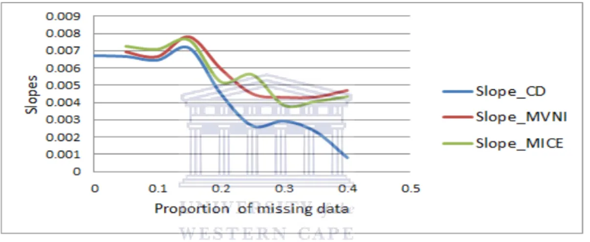
3.1 Estimates of slopes for age when the CD, MVNI and MICE methods are used at different rates of missingness . . . 57
3.2 Estimates of slopes for education when the CD, MVNI and MICE methods are used at different rates of missingness . . . 57
3.3 Estimates of standard errors for age when the CD, MVNI and MICE methods are used at different rates of missingness . . . 57
3.4 Estimates of standard errors for education when the CD, MVNI and MICE methods are used at different rates of missingness . . . . 58
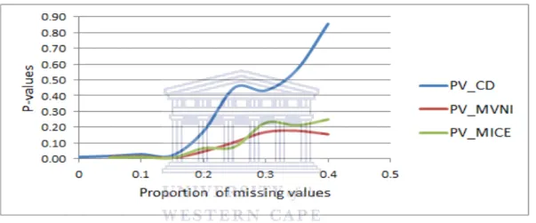
3.5 P-values of the models estimated using the CD, MVNI and MICE methods at different rates of missingness . . . 58
x
List of figures xi
4.1 Missing data models considered in the analysis. . . 67
5.1 Scenario 1: Logistic regression models with missing values on the covariates. . . 78
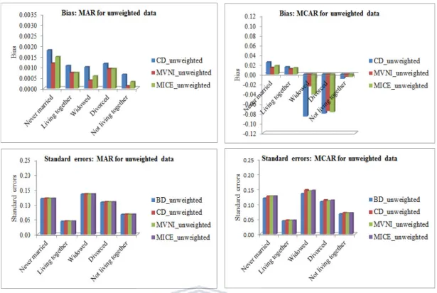
5.2 Model 1.1: Plot of bias and standard errors when 50% data are MAR or MCAR on marital status for unweighted data sets. . . 85
5.3 Model 1.1: Plot of bias and standard errors when 50% data are MAR or MCAR on marital status for weighted data sets. . . 85
5.4 Model 1.1: Plot of bias and standard errors when approximately 30% data are MAR and MCAR for unweighted data sets. . . 92
5.5 Model 1.1: Plot of bias and standard errors when approximately 30% data are MAR and MCAR for weighted data sets. . . 92
5.6 Model 1.1: Plot of bias and standard errors when 10% of the data are MAR and MCAR for unweighted data sets. . . 99
5.7 Model 1.1: Plot of bias and standard errors when 10% of the data are MAR and MCAR for weighted data sets. . . 99
5.8 Model 1.2.1: Plot of bias and standard errors when 50% of the data are MAR and MCAR for unweighted data sets. Numbers 1-5 and 6-15 refer to levels or categories of the variable marital status and region respectively. . . 107
5.9 Model 1.2.1: Plot of bias and standard errors when 50% of the data are MAR and MCAR for weighted data sets. Numbers 1-5 and 6-15 refer to levels or categories of the variable marital status and region respectively. . . 107
5.10 Model 1.2.1: Plot of bias and standard errors when 50% of the data are MAR and MCAR for unweighted data sets. Numbers 1-5 and 6-15 refer to levels or categories of the variable marital status and region respectively, 16-17 refer to variables age and education respectively, and 18-21 refer to levels of wealth index. . . 114
5.11 Model 1.2.1: Plot of bias and standard errors when 50% of the data are MAR and MCAR for weighted data sets. Numbers 1-5 and 6-15 refer to levels or categories of the variable marital status and region respectively, 16-17 refer to variables age and education respectively, and 18-21 refer to levels of wealth index. . . 115
5.12 Scenario 2: Logistic regression models with missing variables on the response variables. . . 118
5.13 Model 2: Plot of bias and standard errors when 50% of the data are MAR and MCAR for unweighted data sets. . . 125
5.14 Model 2: Plot of bias and standard errors when 50% of the data are MAR or MCAR for weighted data sets. . . 125
5.15 Model 2.2: Plot of bias and standard errors of the traditional method use category when 50% data are MAR and MCAR for unweighted data sets. . . 135
5.16 Model 2.2: Plot of bias and standard errors of the traditional method use category when 50% data are MAR and MCAR for weighted data sets. . . 135
5.17 Model 2.2: Plot of bias and standard errors of the modern method use category when 50% data are MAR and MCAR for unweighted data sets. . . 136
5.18 Model 2.2: Plot of bias and standard errors of the modern method use category when 50% data are MAR and MCAR for weighted data sets. . . 136
6.1 Model 1.1: Independent-samples t-test to compare age (in V012) for missing (coded 1 in the table) and present or not missing (coded 0) under MAR assumption. . . 158
6.2 Model 1.1: Independent-samples t-test to compare education in completed years (V133) for missing (coded 1 in the table) and present or not missing (coded 0) under MAR assumption.. . . 159
6.3 Model 1.1: Independent-samples t-test to compare age (V012) for missing (coded 1 in the table) and present or not missing (coded 0) under MCAR assumption. . . 160
6.4 Model 1.1: Independent-samples t-test to compare education in completed years (V133) for missing (coded 1 in the table) and present or not missing (coded 0) under MCAR assumption. . . 161
6.5 Model 1.1: Independent-samples t-test to compare age (in V012) for missing (coded 1 in the table) and present or not missing (coded 0) under MAR assumption. . . 162
6.6 Model 1.1: Independent-samples t-test to compare education in completed years (V133) for missing (coded 1 in the table) and present or not missing (coded 0) under MAR assumption.. . . 163
6.7 Model 1.1: Independent-samples t-test to compare age (V012) for missing (coded 1 in the table) and present or not missing (coded 0) under MCAR assumption. . . 164
6.8 Model 1.1: Independent-samples t-test to compare education in completed years (V133) for missing (coded 1 in the table) and present or not missing (coded 0) under MCAR assumption. . . 165
6.9 Model 1.1: Independent-samples t-test to compare age (in V012) for missing (coded 1 in the table) and present or not missing (coded 0) under MAR assumption under MAR assumption. . . 166
6.10 Model 1.1: Independent-samples t-test to compare education in completed years (V133) for missing (coded 1 in the table) and present or not missing (coded 0) under MAR assumption.. . . 167
6.11 Model 1.1: Independent-samples t-test to compare age (V012) for missing (coded 1 in the table) and present or not missing (coded 0) under MCAR assumption. . . 168
6.12 Model 1.1: Independent-samples t-test to compare education in completed years (V133) for missing (coded 1 in the table) and present or not missing (coded 0) under MCAR assumption. . . 169
6.13 Model 1.2.1: Independent-samples t-test to compare age (in V012) for missing (coded 1 in the table) and present or not missing (coded 0) under MAR assumption. . . 170
List of figures xiii
6.14 Model 1.2.1: Independent-samples t-test to compare education in completed years (V133) for missing (coded 1 in the table) and present or not missing (coded 0) under MAR assumption.. . . 171
6.15 Model 1.2.1: Independent-samples t-test to compare age (V012) for missing (coded 1 in the table) and present or not missing (coded 0) under MCAR assumption. . . 172
6.16 Model 1.2.1: Independent-samples t-test to compare education in completed years (V133) for missing (coded 1 in the table) and present or not missing (coded 0) under MCAR assumption. . . 173
6.17 Model 2.1: Independent-samples t-test to compare age (in V012) for missing (coded 1 in the table) and present or not missing (coded 0) under MAR assumption. . . 174
6.18 Model 2.1: Independent-samples t-test to compare education in completed years (V133) for missing (coded 1 in the table) and present or not missing (coded 0) under MAR assumption.. . . 175
6.19 Model 2.1: Independent-samples t-test to compare age (in V012) for missing (coded 1 in the table) and present or not missing (coded 0) under MAR assumption. . . 176
6.20 Model 2.1: Independent-samples t-test to compare education in completed years (V133) for missing (coded 1 in the table) and present or not missing (coded 0) under MAR assumption.. . . 177
6.21 Model 2.1: Independent-samples t-test to compare age (in V012) for missing (coded 1 in the table) and present or not missing (coded 0) under MAR assumption. . . 178
6.22 Model 2.1: Independent-samples t-test to compare education in completed years (V133) for missing (coded 1 in the table) and present or not missing (coded 0) under MAR assumption.. . . 179
6.23 Model 2.1: Independent-samples t-test to compare age (in V012) for missing (coded 1 in the table) and present or not missing (coded 0) under MAR assumption. . . 180
6.24 Model 2.1: Independent-samples t-test to compare education in completed years (V133) for missing (coded 1 in the table) and present or not missing (coded 0) under MAR assumption.. . . 181
6.25 Model 1.1: Convergence of MCMC after MVNI under MAR as-sumption on marital status: plot of the estimates of WLF against the iteration numbers for unweighted data set. . . 213
6.26 Model 1.1: Convergence of MCMC after MVNI under MAR as-sumption on marital status: plot of the estimates of WLF versus the lag numbers for unweighted data set. . . 213
6.27 Model 1.1: Convergence of MCMC after MICE under MAR as-sumption on marital status: plot of the estimates of WLF against the iteration numbers for unweighted data set. . . 214
6.28 Model 1.1: Convergence of MCMC after MICE under MAR as-sumption on marital status: plot of the estimates of WLF versus the lag numbers for unweighted data set. . . 214
6.29 Model 1.1: Convergence of MCMC after MVNI under MCAR as-sumption on marital status: plot of the estimates of WLF against the iteration numbers for unweighted data set. . . 215
6.30 Model 1.1: Convergence of MCMC after MVNI under MCAR as-sumption on marital status: plot of the estimates of WLF versus the lag numbers for unweighted data set. . . 215
6.31 Model 1.1: Convergence of MCMC after MICE under MCAR as-sumption on marital status: plot of the estimates of WLF against the iteration numbers for unweighted data set. . . 216
6.32 Model 1.1: Convergence of MCMC after MICE under MCAR as-sumption on marital status: plot of the estimates of WLF versus the lag numbers for unweighted data set. . . 216
6.33 Model 1.1: Convergence of MCMC after MVNI under MAR as-sumption on marital status: plot of the estimates of WLF against the iteration numbers for weighted data set. . . 217
6.34 Model 1.1: Convergence of MCMC after MVNI under MAR as-sumption on marital status: plot of the estimates of WLF versus the lag numbers for weighted data set. . . 217
6.35 Model 1.1: Convergence of MCMC after MICE under MAR as-sumption on marital status: plot of the estimates of WLF against the iteration numbers for weighted data set. . . 218
6.36 Model 1.1: Convergence of MCMC after MICE under MAR as-sumption on marital status: plot of the estimates of WLF versus the lag numbers for weighted data set. . . 218
6.37 Model 1.1: Convergence of MCMC after MVNI under MCAR as-sumption on marital status: plot of the estimates of WLF against the iteration numbers for weighted data set. . . 219
6.38 Model 1.1: Convergence of MCMC after MVNI under MCAR as-sumption on marital status: plot of the estimates of WLF versus the lag numbers for weighted data set. . . 219
6.39 Model 1.1: Convergence of MCMC after MICE under MCAR as-sumption on marital status: plot of the estimates of WLF against the iteration numbers for weighted data set. . . 220
6.40 Model 1.1: Convergence of MCMC after MICE under MCAR as-sumption on marital status: plot of the estimates of WLF versus the lag numbers for weighted data set. . . 220
6.41 Model 1.1: Convergence of MCMC after MVNI under MAR as-sumption on marital status: plot of the estimates of WLF against the iteration numbers for unweighted data set. . . 221
6.42 Model 1.1: Convergence of MCMC after MVNI under MAR as-sumption on marital status: plot of the estimates of WLF versus the lag numbers for unweighted data set . . . 221
6.43 Model 1.1: Convergence of MCMC after MICE under MAR as-sumption on marital status: plot of the estimates of WLF against the iteration numbers for unweighted data set . . . 222
List of figures xv
6.44 Model 1.1: Convergence of MCMC after MICE under MAR as-sumption on marital status: plot of the estimates of WLF versus the lag numbers for unweighted data set . . . 222
6.45 Model 1.1: Convergence of MCMC after MVNI under MCAR as-sumption on marital status: plot of the estimates of WLF against the iteration numbers for unweighted data set. . . 223
6.46 Model 1.1: Convergence of MCMC after MVNI under MCAR as-sumption on marital status: plot of the estimates of WLF versus the lag numbers for unweighted data set . . . 223
6.47 Model 1.1: Convergence of MCMC after MICE under MCAR as-sumption on marital status: plot of the estimates of WLF against the iteration numbers for unweighted data set . . . 224
6.48 Model 1.1: Convergence of MCMC after MICE under MCAR as-sumption on marital status: plot of the estimates of WLF versus the lag numbers for unweighted data set . . . 224
6.49 Model 1.1: Convergence of MCMC after MVNI under MAR as-sumption on marital status: plot of the estimates of WLF against the iteration numbers for weighted data set. . . 225
6.50 Model 1.1: Convergence of MCMC after MVNI under MAR as-sumption on marital status: plot of the estimates of WLF versus the lag numbers for weighted data set. . . 225
6.51 Model 1.1: Convergence of MCMC after MICE under MAR as-sumption on marital status: plot of the estimates of WLF against the iteration numbers for weighted data set. . . 226
6.52 Model 1.1: Convergence of MCMC after MICE under MAR as-sumption on marital status: plot of the estimates of WLF versus the lag numbers for weighted data set . . . 226
6.53 Model 1.1: Convergence of MCMC after MVNI under MCAR as-sumption on marital status: plot of the estimates of WLF against the iteration numbers for weighted data set. . . 227
6.54 Model 1.1: Convergence of MCMC after MVNI under MCAR as-sumption on marital status: plot of the estimates of WLF versus the lag numbers for weighted data set. . . 227
6.55 Model 1.1: Convergence of MCMC after MICE under MCAR as-sumption on marital status: plot of the estimates of WLF against the iteration numbers for weighted data set. . . 228
6.56 Model 1.1: Convergence of MCMC after MICE under MCAR as-sumption on marital status: plot of the estimates of WLF versus the lag numbers for weighted data set . . . 228
6.57 Model 1.1: Convergence of MCMC after MVNI under MAR as-sumption on marital status: plot of the estimates of WLF against the iteration numbers for unweighted data set. . . 229
6.58 Model 1.1: Convergence of MCMC after MVNI under MAR as-sumption on marital status: plot of the estimates of WLF versus the lag numbers for unweighted data set. . . 229
6.59 Model 1.1: Convergence of MCMC after MICE under MAR as-sumption on marital status: plot of the estimates of WLF against the iteration numbers for unweighted data set. . . 230
6.60 Model 1.1: Convergence of MCMC after MICE under MAR as-sumption on marital status: plot of the estimates of WLF versus the lag numbers for unweighted data set. . . 230
6.61 Model 1.1: Convergence of MCMC after MVNI under MCAR as-sumption on marital status: plot of the estimates of WLF against the iteration numbers for unweighted data set. . . 231
6.62 Model 1.1: Convergence of MCMC after MVNI under MCAR as-sumption on marital status: plot of the estimates of WLF versus the lag numbers for unweighted data set. . . 231
6.63 Model 1.1: Convergence of MCMC after MICE under MCAR as-sumption on marital status: plot of the estimates of WLF against the iteration numbers for unweighted data set. . . 232
6.64 Model 1.1: Convergence of MCMC after MICE under MCAR as-sumption on marital status: plot of the estimates of WLF versus the lag numbers for unweighted data set. . . 232
6.65 Model 1.1: Convergence of MCMC after MVNI under MAR as-sumption on marital status: plot of the estimates of WLF against the iteration numbers for weighted data set. . . 233
6.66 Model 1.1: Convergence of MCMC after MVNI under MAR as-sumption on marital status: plot of the estimates of WLF versus the lag numbers for weighted data set. . . 233
6.67 Model 1.1: Convergence of MCMC after MICE under MAR as-sumption on marital status: plot of the estimates of WLF against the iteration numbers for weighted data set. . . 234
6.68 Model 1.1: Convergence of MCMC after MICE under MAR as-sumption on marital status: plot of the estimates of WLF versus the lag numbers for weighted data set. . . 234
6.69 Model 1.1: Convergence of MCMC after MVNI under MCAR as-sumption on marital status: plot of the estimates of WLF against the iteration numbers for weighted data set. . . 235
6.70 Model 1.1: Convergence of MCMC after MVNI under MCAR as-sumption on marital status: plot of the estimates of WLF versus the lag numbers for weighted data set. . . 235
6.71 Model 1.1: Convergence of MCMC after MICE under MCAR as-sumption on marital status: plot of the estimates of WLF against the iteration numbers for weighted data set. . . 236
6.72 Model 1.1: Convergence of MCMC after MICE under MCAR as-sumption on marital status: plot of the estimates of WLF versus the lag numbers for weighted data set. . . 236
6.73 Model 1.2.1: Convergence of MCMC after MVNI under MAR as-sumption on marital status: plot of the estimates of WLF against the iteration numbers for unweighted data set. . . 237
List of figures xvii
6.74 Model 1.2.1: Convergence of MCMC after MVNI under MAR as-sumption on marital status: plot of the estimates of WLF versus the lag numbers for unweighted data set. . . 237
6.75 Model 1.2.1: Convergence of MCMC after MICE under MAR as-sumption on marital status: plot of the estimates of WLF against the iteration numbers for unweighted data set. . . 238
6.76 Model 1.2.1: Convergence of MCMC after MICE under MAR as-sumption on marital status: plot of the estimates of WLF versus the lag numbers for unweighted data set. . . 238
6.77 Model 1.2.1: Convergence of MCMC after MVNI under MCAR assumption on marital status: plot of the estimates of WLF against the iteration numbers for unweighted data set. . . 239
6.78 Model 1.2.1: Convergence of MCMC after MVNI under MCAR assumption on marital status: plot of the estimates of WLF versus the lag numbers for unweighted data set. . . 239
6.79 Model 1.2.1: Convergence of MCMC after MICE under MCAR assumption on marital status: plot of the estimates of WLF against the iteration numbers for unweighted data set. . . 240
6.80 Model 1.2.1: Convergence of MCMC after MICE under MCAR assumption on marital status: plot of the estimates of WLF versus the lag numbers for unweighted data set. . . 240
6.81 Model 1.2.1: Convergence of MCMC after MVNI under MAR as-sumption on marital status: plot of the estimates of WLF against the iteration numbers for weighted data set. . . 241
6.82 Model 1.2.1: Convergence of MCMC after MVNI under MAR as-sumption on marital status: plot of the estimates of WLF versus the lag numbers for weighted data set. . . 241
6.83 Model 1.2.1: Convergence of MCMC after MICE under MAR as-sumption on marital status: plot of the estimates of WLF against the iteration numbers for weighted data set. . . 242
6.84 Model 1.2.1: Convergence of MCMC after MICE under MAR as-sumption on marital status: plot of the estimates of WLF versus the lag numbers for weighted data set. . . 242
6.85 Model 1.2.1: Convergence of MCMC after MVNI under MCAR assumption on marital status: plot of the estimates of WLF against the iteration numbers for weighted data set. . . 243
6.86 Model 1.2.1: Convergence of MCMC after MVNI under MCAR assumption on marital status: plot of the estimates of WLF versus the lag numbers for weighted data set. . . 243
6.87 Model 1.2.1: Convergence of MCMC after MICE under MCAR assumption on marital status: plot of the estimates of WLF against the iteration numbers for weighted data set. . . 244
6.88 Model 1.2.1: Convergence of MCMC after MICE under MCAR assumption on marital status: plot of the estimates of WLF versus the lag numbers for weighted data set. . . 244
6.89 Model 1.2.2: Convergence of MCMC after MVNI under MAR as-sumption on marital status: plot of the estimates of WLF against the iteration numbers for unweighted data set. . . 245
6.90 Model 1.2.2: Convergence of MCMC after MVNI under MAR as-sumption on marital status: plot of the estimates of WLF versus the lag numbers for unweighted data set. . . 245
6.91 Model 1.2.2: Convergence of MCMC after MICE under MAR as-sumption on marital status: plot of the estimates of WLF against the iteration numbers for unweighted data set. . . 246
6.92 Model 1.2.2: Convergence of MCMC after MICE under MAR as-sumption on marital status: plot of the estimates of WLF versus the lag numbers for unweighted data set. . . 246
6.93 Model 1.2.2: Convergence of MCMC after MVNI under MCAR assumption on marital status: plot of the estimates of WLF against the iteration numbers for unweighted data set. . . 247
6.94 Model 1.2.2: Convergence of MCMC after MVNI under MCAR assumption on marital status: plot of the estimates of WLF versus the lag numbers for unweighted data set. . . 247
6.95 Model 1.2.2: Convergence of MCMC after MICE under MCAR assumption on marital status: plot of the estimates of WLF against the iteration numbers for unweighted data set. . . 248
6.96 Model 1.2.2: Convergence of MCMC after MICE under MCAR assumption on marital status: plot of the estimates of WLF versus the lag numbers for unweighted data set. . . 248
6.97 Model 1.2.2: Convergence of MCMC after MVNI under MAR as-sumption on marital status: plot of the estimates of WLF against the iteration numbers for weighted data set. . . 249
6.98 Model 1.2.2: Convergence of MCMC after MVNI under MAR as-sumption on marital status: plot of the estimates of WLF versus the lag numbers for weighted data set. . . 249
6.99 Model 1.2.2: Convergence of MCMC after MICE under MAR as-sumption on marital status: plot of the estimates of WLF against the iteration numbers for weighted data set. . . 250
6.100Model 1.2.2: Convergence of MCMC after MICE under MAR as-sumption on marital status: plot of the estimates of WLF versus the lag numbers for weighted data set. . . 250
6.101Model 1.2.2: Convergence of MCMC after MVNI under MCAR assumption on marital status: plot of the estimates of WLF against the iteration numbers for weighted data set. . . 251
6.102Model 1.2.2: Convergence of MCMC after MVNI under MCAR assumption on marital status: plot of the estimates of WLF versus the lag numbers for weighted data set. . . 251
6.103Model 1.2.2: Convergence of MCMC after MICE under MCAR assumption on marital status: plot of the estimates of WLF against the iteration numbers for weighted data set. . . 252
List of figures xix
6.104Model 1.2.2: Convergence of MCMC after MICE under MCAR assumption on marital status: plot of the estimates of WLF versus the lag numbers for weighted data set. . . 252
6.105Model 2.1: Convergence of MCMC after MVNI under MAR as-sumption on contraceptive method use status (dichotomous vari-able): plot of the estimates of WLF against the iteration numbers for unweighted data set. . . 253
6.106Model 2.1: Convergence of MCMC after MVNI under MAR as-sumption on contraceptive method use status (dichotomous vari-able): plot of the estimates of WLF versus the lag numbers for unweighted data set. . . 253
6.107Model 2.1: Convergence of MCMC after MICE under MAR as-sumption on contraceptive method use status (dichotomous vari-able): plot of the estimates of WLF against the iteration numbers for unweighted data set. . . 254
6.108Model 2.1: Convergence of MCMC after MICE under MAR as-sumption on contraceptive method use status (dichotomous vari-able): plot of the estimates of WLF versus the lag numbers for unweighted data set. . . 254
6.109Model 2.1: Convergence of MCMC after MVNI under MCAR as-sumption on contraceptive method use status (dichotomous vari-able): plot of the estimates of WLF against the iteration numbers for unweighted data set. . . 255
6.110Model 2.1: Convergence of MCMC after MVNI under MCAR as-sumption on contraceptive method use status (dichotomous vari-able): plot of the estimates of WLF versus the lag numbers for unweighted data set. . . 255
6.111Model 2.1: Convergence of MCMC after MICE under MCAR as-sumption on contraceptive method use status (dichotomous vari-able): plot of the estimates of WLF against the iteration numbers for unweighted data set. . . 256
6.112Model 2.1: Convergence of MCMC after MICE under MCAR as-sumption on contraceptive method use status (dichotomous vari-able): plot of the estimates of WLF versus the lag numbers for unweighted data set. . . 256
6.113Model 2.1: Convergence of MCMC after MVNI under MAR as-sumption on contraceptive method use status (dichotomous vari-able): plot of the estimates of WLF against the iteration numbers for weighted data set. . . 257
6.114Model 2.1: Convergence of MCMC after MVNI under MAR as-sumption on contraceptive method use status (dichotomous vari-able): plot of the estimates of WLF versus the lag numbers for weighted data set.. . . 257
6.115Model 2.1: Convergence of MCMC after MICE under MAR as-sumption on contraceptive method use status (dichotomous vari-able): plot of the estimates of WLF against the iteration numbers for weighted data set. . . 258
6.116Model 2.1: Convergence of MCMC after MICE under MAR as-sumption on contraceptive method use status (dichotomous vari-able): plot of the estimates of WLF versus the lag numbers for weighted data set.. . . 258
6.117Model 2.1: Convergence of MCMC after MVNI under MCAR as-sumption on contraceptive method use status (dichotomous vari-able): plot of the estimates of WLF against the iteration numbers for weighted data set. . . 259
6.118Model 2.1: Convergence of MCMC after MVNI under MCAR as-sumption on contraceptive method use status (dichotomous vari-able): plot of the estimates of WLF versus the lag numbers for weighted data set.. . . 259
6.119Model 2.1: Convergence of MCMC after MICE under MCAR as-sumption on contraceptive method use status (dichotomous vari-able): plot of the estimates of WLF against the iteration numbers for weighted data set. . . 260
6.120Model 2.1: Convergence of MCMC after MICE under MCAR as-sumption on contraceptive method use status (dichotomous vari-able): plot of the estimates of WLF versus the lag numbers for weighted data set.. . . 260
6.121Model 2.2: Convergence of MCMC after MVNI under MAR as-sumption on contraceptive method use status (dichotomous vari-able): plot of the estimates of WLF against the iteration numbers for unweighted data set. . . 261
6.122Model 2.2: Convergence of MCMC after MVNI under MAR as-sumption on contraceptive method use status (dichotomous vari-able): plot of the estimates of WLF versus the lag numbers for unweighted data set. . . 261
6.123Model 2.2: Convergence of MCMC after MICE under MAR as-sumption on contraceptive method use status (dichotomous vari-able): plot of the estimates of WLF against the iteration numbers for unweighted data set. . . 262
6.124Model 2.2: Convergence of MCMC after MICE under MAR as-sumption on contraceptive method use status (dichotomous vari-able): plot of the estimates of WLF versus the lag numbers for unweighted data set. . . 262
6.125Model 2.2: Convergence of MCMC after MVNI under MCAR as-sumption on contraceptive method use status (dichotomous vari-able): plot of the estimates of WLF against the iteration numbers for unweighted data set. . . 263
List of figures xxi
6.126Model 2.2: Convergence of MCMC after MVNI under MCAR as-sumption on contraceptive method use status (dichotomous vari-able): plot of the estimates of WLF versus the lag numbers for unweighted data set. . . 263
6.127Model 2.2: Convergence of MCMC after MICE under MCAR as-sumption on contraceptive method use status (dichotomous vari-able): plot of the estimates of WLF against the iteration numbers for unweighted data set. . . 264
6.128Model 2.2: Convergence of MCMC after MICE under MCAR as-sumption on contraceptive method use status (dichotomous vari-able): plot of the estimates of WLF versus the lag numbers for unweighted data set. . . 264
6.129Model 2.2: Convergence of MCMC after MVNI under MAR as-sumption on contraceptive method use status (dichotomous vari-able): plot of the estimates of WLF against the iteration numbers for weighted data set. . . 265
6.130Model 2.2: Convergence of MCMC after MVNI under MAR as-sumption on contraceptive method use status (dichotomous vari-able): plot of the estimates of WLF versus the lag numbers for weighted data set.. . . 265
6.131Model 2.2: Convergence of MCMC after MICE under MAR as-sumption on contraceptive method use status (dichotomous vari-able): plot of the estimates of WLF against the iteration numbers for weighted data set. . . 266
6.132Model 2.2: Convergence of MCMC after MICE under MAR as-sumption on contraceptive method use status (dichotomous vari-able): plot of the estimates of WLF versus the lag numbers for weighted data set.. . . 266
6.133Model 2.2: Convergence of MCMC after MVNI under MCAR as-sumption on contraceptive method use status (dichotomous vari-able): plot of the estimates of WLF against the iteration numbers for weighted data set. . . 267
6.134Model 2.2: Convergence of MCMC after MVNI under MCAR as-sumption on contraceptive method use status (dichotomous vari-able): plot of the estimates of WLF versus the lag numbers for weighted data set.. . . 267
6.135Model 2.2: Convergence of MCMC after MICE under MCAR as-sumption on contraceptive method use status (dichotomous vari-able): plot of the estimates of WLF against the iteration numbers for weighted data set. . . 268
6.136Model 2.2: Convergence of MCMC after MICE under MCAR as-sumption on contraceptive method use status (dichotomous vari-able): plot of the estimates of WLF versus the lag numbers for weighted data set.. . . 268
List of Tables
3.1 Imputation of categorical variables with more than two levels . . . 47
3.2 Parameter estimates of a set of logistic regression models for predict-ing the contraceptive methods use status by women of reproductive age in Democratic Republic of Congo in 2007, using age (1st covari-ate) and education (2nd covariate) in years as explanatory variables 56
4.1 Description of the variables used in the study . . . 64
5.1 Model 1.1: Frequency distribution of missingness on marital status under MAR assumption. . . 79
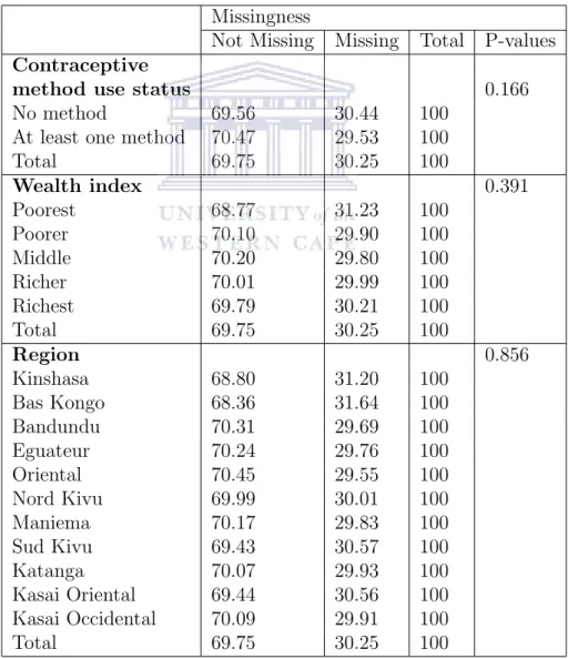
5.2 Model 1.1: Distribution of missingness across selected categorical variables when 50% data are MAR on marital status if a woman is not using any contraceptive method. . . 80
5.3 Model 1.1: Frequency distribution of missingness when 50% data are MCAR on marital status. . . 81
5.4 Model 1.1: Distribution of missingness by selected categorical vari-ables when 50% data are MCAR on marital status. . . 82
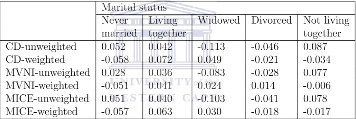
5.5 Model 1.1: Estimates of bias when approximately 50% of data are MAR on marital status if a woman is not using any contraceptive method. . . 83
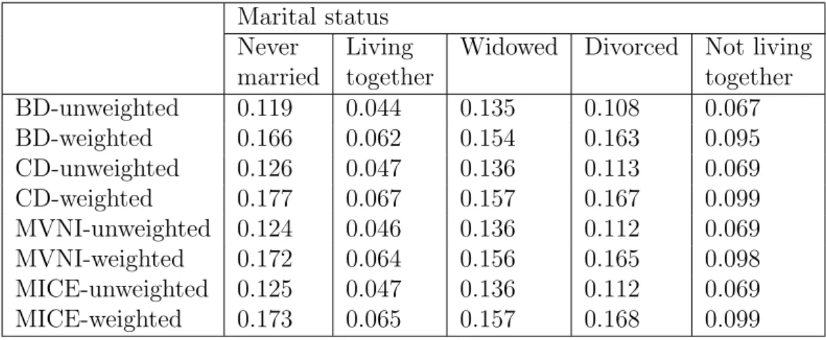
5.6 Model 1.1: Estimates of standard errors when approximately 50% of data are MAR on marital status if a woman is not using any contraceptive method. . . 84
5.7 Model 1.1: Estimates of bias when approximately 50% of data are MCAR on marital status. . . 84
5.8 Model 1.1: Estimates of standard errors when approximately 50% of data are MCAR on marital status. . . 84
5.9 Model 1.1: Frequency distribution of missingness when approxi-mately 50% data are MAR on marital status if a woman is not using any contraceptive method. . . 87
5.10 Model 1.1: Distribution of missingness across selected categorical variables when approximately 30% data are MAR on marital status if a woman is not using any contraceptive method.. . . 88
5.11 Model 1.1: Frequency distribution of missingness when approxi-mately 30% data are MCAR on marital status. . . 88
5.12 Model 1.1: Distribution of missingness by selected categorical vari-ables when approximately 30% data are MCAR on marital status. . 89
xxii
List of tables xxiii
5.13 Model 1.1: Estimates of bias when approximately 30% of data are MAR on marital status if a woman is not using any contraceptive method. . . 90
5.14 Model 1.1: Estimates of standard errors when approximately 30% of data are MAR on marital status if a woman is not using any contraceptive method. . . 91
5.15 Model 1.1: Estimates of bias when approximately 30% of data are MCAR on marital status. . . 91
5.16 Model 1.1: Estimates of standard errors when approximately 30% of data are MCAR on marital status. . . 91
5.17 Model 1.1: Frequency distribution of missingness when approxi-mately 10% of the data are MAR on marital status if a woman is not using any contraceptive method. . . 94
5.18 Model 1: Distribution of missingness across selected categorical variables when approximately 10% of the data are MAR on marital status if a woman is not using any contraceptive method. . . 95
5.19 Model 1.1: Frequency distribution of missingness when approxi-mately 10% of the data are MCAR on marital status. . . 95
5.20 Model 1: Distribution of missingness by selected categorical vari-ables when approximately 10% of the data are MCAR on marital status. . . 96
5.21 Model 1.1: Estimates of bias when approximately 10% of the data are MAR on marital status if a woman is not using any contraceptive method. . . 97
5.22 Model 1.1: Estimates of standard errors when approximately 10% of the data are MAR on marital status if a woman is not using any contraceptive method. . . 98
5.23 Model 1.1: Estimates of bias when approximately 10% of the data are MCAR on marital status. . . 98
5.24 Model 1.1: Estimates of standard errors when approximately 10% of the data are MCAR on marital status. . . 98
5.25 Model 1.2.1: Frequency distribution of missingness when 50% of the data are MAR on marital status and region if a woman is not using any contraceptive method. . . 101
5.26 Model 1.2.1: Distribution of missingness across selected categorical when 50% of the data are MAR on marital status and region if a woman is not using any contraceptive method. . . 102
5.27 Model 1.2.1: Frequency distribution of missingness when 50% of the data are MCAR on marital status and region. . . 102
5.28 Model 1.2.1: Distribution of missingness when 50% of the data are MCAR on marital status and region. . . 103
5.29 Model 1.2.1: Estimates of bias and standard errors (SE) obtained when 50% of the data are MAR on variables marital status and region if a woman is not using any contraceptive method: results from the unweighted data set. . . 104
5.30 Model 1.2.1: Estimates of bias and standard errors (SE) obtained when 50% of the data are MAR on variables marital status and region if a woman is not using any contraceptive method: results from the weighted data. . . 105
5.31 Model 1.2.1: Estimates of bias and standard errors (SE) obtained when 50% of the data are MCAR on variables marital status and region: results from the unweighted data set. . . 105
5.32 Model 1.2.1: Estimates of bias and standard errors (SE) obtained when 50% of the data are MCAR on variables marital status and region: results from the weighted data set. . . 106
5.33 Model 1.2.2: Estimates of bias and standard errors (SE) obtained when 50% of the data are MAR on variables marital status and region if a woman is not using any contraceptive method: results from the unweighted data set. . . 110
5.34 Model 1.2.2: Estimates of bias and standard errors (SE) obtained when 50% of the data are MAR on variables marital status and region if a woman is not using any contraceptive method: results from the weighted data set. . . 111
5.35 Model 1.2.2: Estimates of bias and standard errors (SE) obtained when 50% of the data are MCAR on variables marital status and region: results from the unweighted data set. . . 112
5.36 Model 1.2.2: Estimates of bias and standard errors (SE) obtained when 50% of the data are MCAR on variables marital status and region: results from the weighted data set. . . 113
5.37 Model 2.1: Frequency distribution of missingness when 50% of the data are MAR on contraceptive method use status if a woman is aged at least 35 years. . . 119
5.38 Model 2.1: Distribution of missingness across categorical variables when 50% of the data are MAR on contraceptive method use status if a woman is aged at least 35 years.. . . 120
5.39 Model 2.1: Frequency distribution of missingness when 50% of the data are MCAR on contraceptive method use status. . . 121
5.40 Model 2.1: Distribution of missingness across marital status when 50% of the data are MCAR on contraceptive method use status. . . 122
5.41 Model 2.1: Estimates of bias when approximately 50% of the data are MAR on contraceptive method use status if a woman is aged at least 35 years. . . 123
5.42 Model 2.1: Estimates of standard errors when approximately 50% of the data are MAR on contraceptive method use status if a woman is aged 35 years or more. . . 123
5.43 Model 2.1: Estimates of bias when approximately 50% of the data are MCAR on contraceptive method use status. . . 124
5.44 Model 2.1: Estimates of standard errors when approximately 50% of the data are MCAR on contraceptive method use status. . . 124
List of tables xxv
5.45 Model 2.2: Frequency distribution of missingness when 50% of the data are MAR on contraceptive method use status if a woman is at least 35 years old. . . 127
5.46 Model 2.2: Distribution of missingness by marital status when ap-proximately 50% of the data are MAR on contraceptive method use status if a woman is at least 35 years old. . . 128
5.47 Model 2.2: Frequency distribution of missingness when 50% of the data are MCAR on contraceptive method use status . . . 128
5.48 Model 2.2: Distribution of missingness by selected categorical vari-ables when 50% data are MCAR on contraceptive methods use status.129
5.49 Model 2.2: Estimates of bias in the regression coefficients of tradi-tional and modern contraceptive methods when approximately 50% of data are MAR on contraceptive method use status if a woman is aged at least 35 years. . . 131
5.50 Model 2.2: Estimates of standard errors of the regression coeffi-cients of traditional and modern contraceptive methods when ap-proximately 50% of data are MAR on contraceptive method use status if a woman is aged at least 35 years. . . 132
5.51 Model 2.2: Estimates of bias in the regression coefficients of tradi-tional and modern contraceptive methods when approximately 50% of data are MCAR on contraceptive method use status. . . 133
5.52 Model 2.2: Estimates of standard errors of the regression coeffi-cients of traditional and modern contraceptive methods when ap-proximately 50% of data are MCAR on contraceptive method use status. . . 134
6.1 Model 1.1: Estimates of Monte Carlo errors after MVNI is applied to unweighted data set with approximately 50% MAR data on mar-ital status if a woman is not using any contraceptive method.. . . . 183
6.2 Model 1.1: Estimates of Monte Carlo errors after MVNI is applied to weighted data set with approximately 50% MAR data on marital status if a woman is not using any contraceptive method. . . 183
6.3 Model 1.1: Estimates of Monte Carlo errors after MICE is applied to unweighted data set with approximately 50% MAR data on marital status if a woman is not using any contraceptive method. . . 184
6.4 Model 1.1: Estimates of Monte Carlo errors after MICE is applied to weighted data set with approximately 50% MAR data on marital status if a woman is not using any contraceptive method. . . 184
6.5 Model 1.1: Estimates of Monte Carlo errors after MVNI is applied to unweighted data set with approximately 50% MCAR data on marital status.. . . 184
6.6 Model 1.1: Estimates of Monte Carlo errors after MVNI is applied to weighted data set with approximately 50% MCAR data on mar-ital status. . . 185
6.7 Model 1.1: Estimates of Monte Carlo errors after MICE is applied to unweighted data set with approximately 50% MCAR data on marital status.. . . 185
6.8 Model 1.1: Estimates of Monte Carlo errors after MICE is applied to weighted data set with approximately 50% MCAR data on marital status. . . 185
6.9 Model 1.1: Estimates of Monte Carlo errors after MVNI is applied to unweighted data set with approximately 30% MAR data on mar-ital status if a woman is not using any contraceptive method.. . . . 186
6.10 Model 1.1: Estimates of Monte Carlo errors after MVNI is applied to weighted data set with approximately 30% MAR data on marital status if a woman is not using any contraceptive method. . . 186
6.11 Model 1.1: Estimates of Monte Carlo errors after MICE is applied to unweighted data set with approximately 30% MAR data on marital status if a woman is not using any contraceptive method. . . 186
6.12 Model 1.1: Estimates of Monte Carlo errors after MICE is applied to weighted data set with approximately 30% MAR data on marital status if a woman is not using any contraceptive method. . . 187
6.13 Model 1.1: Estimates of Monte Carlo errors after MVNI is applied to unweighted data set with approximately 30% MCAR data on marital status.. . . 187
6.14 Model 1.1: Estimates of Monte Carlo errors after MVNI is applied to weighted data set with approximately 30% MCAR data on mar-ital status. . . 187
6.15 Model 1.1: Estimates of Monte Carlo errors after MICE is applied to unweighted data set with approximately 30% MCAR data on marital status.. . . 188
6.16 Model 1.1: Estimates of Monte Carlo errors after MICE is applied to weighted data set with approximately 30% MCAR data on marital status. . . 188
6.17 Model 1.1: Estimates of Monte Carlo errors after MVNI is applied to unweighted data set with approximately 10% MAR data on mar-ital status if a woman is not using any contraceptive method.. . . . 189
6.18 Model 1.1: Estimates of Monte Carlo errors after MVNI is applied to weighted data set with approximately 10% MAR data on marital status if a woman is not using any contraceptive method. . . 189
6.19 Model 1.1: Estimates of Monte Carlo errors after MICE is applied to unweighted data set with approximately 10% MAR data on marital status if a woman is not using any contraceptive method. . . 189
6.20 Model 1.1: Estimates of Monte Carlo errors after MICE is applied to weighted data set with approximately 10% MAR data on marital status if a woman is not using any contraceptive method. . . 190
6.21 Model 1.1: Estimates of Monte Carlo errors after MVNI is applied to unweighted data set with approximately 10% MCAR data on marital status.. . . 190
List of tables xxvii
6.22 Model 1.1: Estimates of Monte Carlo errors after MVNI is applied to weighted data set with approximately 10% MCAR data on mar-ital status. . . 190
6.23 Model 1.1: Estimates of Monte Carlo errors after MICE is applied to unweighted data set with approximately 10% MCAR data on marital status.. . . 191
6.24 Model 1.1: Estimates of Monte Carlo errors after MICE is applied to weighted data set with approximately 10% MCAR data on marital status. . . 191
6.25 Model 1.2.1: Estimates of Monte Carlo errors after MVNI is ap-plied to unweighted data set with approximately 50% MAR data on marital status and region if a woman is not using any contra-ceptive method. . . 192
6.26 Model 1.2.1: Estimates of Monte Carlo errors after MVNI is applied to weighted data set with approximately 50% MAR data on marital status and region if a woman is not using any contraceptive method.193
6.27 Model 1.2.1: Estimates of Monte Carlo errors after MICE is ap-plied to unweighted data set with approximately 50% MAR data on marital status and region if a woman is not using any contra-ceptive method. . . 193
6.28 Model 1.2.1: Estimates of Monte Carlo errors after MICE is applied to weighted data set with approximately 50% MAR data on marital status and region if a woman is not using any contraceptive method.194
6.29 Model 1.2.1: Estimates of Monte Carlo errors after MVNI is applied to unweighted data set with approximately 50% MCAR data on marital status and region. . . 194
6.30 Model 1.2.1: Estimates of Monte Carlo errors after MVNI is ap-plied to weighted data set with approximately 50% MCAR data on marital status and region. . . 195
6.31 Model 1.2.1: Estimates of Monte Carlo errors after MICE is applied to unweighted data set with approximately 50% MCAR data on marital status and region. . . 195
6.32 Model 1.2.1: Estimates of Monte Carlo errors after MICE is ap-plied to weighted data set with approximately 50% MCAR data on marital status and region. . . 196
6.33 Model 1.2.2: Estimates of Monte Carlo errors after MVNI is applied to unweighted data set with approximately 50% of data missing at random on marital status and region if a woman is not using any contraceptive method. . . 197
6.34 Model 1.2.2: Estimates of Monte Carlo errors after MVNI is applied to weighted data set with approximately 50% of data missing at random on marital status and region if a woman is not using any contraceptive method. . . 198
6.35 Model 1.2.2: Estimates of Monte Carlo errors after MICE is ap-plied to unweighted data set with approximately 50% MAR data on marital status and region is a woman is not using any contra-ceptive method. . . 199
6.36 Model 1.2.2: Estimates of Monte Carlo errors after MICE is applied to weighted data set with approximately 50% MAR data on marital status and region is a woman is not using any contraceptive method.200
6.37 Model 1.2.2: Estimates of Monte Carlo errors after MVNI is applied to unweighted data set with approximately 50% MCAR data on marital status and region. . . 201
6.38 Model 1.2.2: Estimates of Monte Carlo errors after MVNI is ap-plied to weighted data set with approximately 50% MCAR data on marital status and region. . . 202
6.39 Model 1.2.2: Estimates of Monte Carlo errors after MICE is applied to unweighted data set with approximately 50% MCAR data on marital status and region. . . 203
6.40 Model 1.2.2: Estimates of Monte Carlo errors after MICE is ap-plied to weighted data set with approximately 50% MCAR data on marital status and region. . . 204
6.41 Model 2.1: Estimates of Monte Carlo errors after MVNI is applied to unweighted data set with approximately 50% MAR data on con-traceptive method use status if a woman is aged at least 35 years. . 205
6.42 Model 2.1: Estimates of Monte Carlo errors after MVNI is applied to weighted data set with approximately 50% MAR data on con-traceptive method use status if a woman is aged at least 35 years. . 205
6.43 Model 2.1: Estimates of Monte Carlo errors after MICE is applied to unweighted data set with approximately 50% MAR data on con-traceptive method use status if a woman is aged at least 35 years. . 206
6.44 Model 2.1: Estimates of Monte Carlo errors after MICE is applied to weighted data set with approximately 50% MAR data on con-traceptive method use status if a woman is aged at least 35 years. . 206
6.45 Model 2.1: Estimates of Monte Carlo errors after MVNI is applied to unweighted data set with approximately 50% MCAR data on contraceptive method use status. . . 206
6.46 Model 2.1: Estimates of Monte Carlo errors after MVNI is applied to weighted data set with approximately 50% MCAR data on con-traceptive method use status. . . 207
6.47 Model 2.1: Estimates of Monte Carlo errors after MICE is applied to unweighted data set with approximately 50% MCAR data on contraceptive method use status. . . 207
6.48 Model 2.1: Estimates of Monte Carlo errors after MICE is applied to weighted data set with approximately 50% MCAR on contraceptive method use status. . . 207
6.49 Model 2.2: Estimates of Monte Carlo errors after MVNI is applied to unweighted data set with approximately 50% MAR data on con-traceptive method use status if a woman is aged at least 35 years. . 208
List of tables xxix
6.50 Model 2.2: Estimates of Monte Carlo errors after MVNI is applied to weighted data set with approximately 50% MAR data on con-traceptive method use status if a woman is aged at least 35 years. . 208
6.51 Model 2.2: Estimates of Monte Carlo errors after MICE is applied to unweighted data set with approximately 50% MAR data on con-traceptive method use status if a woman is aged at least 35 years. . 209
6.52 Model 2.2: Estimates of Monte Carlo errors after MICE is applied to weighted data set with approximately 50% MAR data on con-traceptive method use status if a woman is aged at least 35 years. . 209
6.53 Model 2.2: Estimates of Monte Carlo errors after MVNI is applied to unweighted data set with approximately 50% MCAR data on contraceptive method use status. . . 210
6.54 Model 2.2: Estimates of Monte Carlo errors after MVNI is applied to weighted data set with approximately 50% MCAR data on con-traceptive method use status. . . 210
6.55 Model 2.2: Estimates of Monte Carlo errors after MICE is applied to unweighted data set with approximately 50% MCAR data on contraceptive methods use status. . . 211
6.56 Model 2.2: Estimates of Monte Carlo errors after MICE is applied to weighted data set with approximately 50% MCAR data on con-traceptive methods use status. . . 211
MCAR Missing completely at random
MAR Missing at random
NMAR Not missing at random
MVN Multivariate normal
MVNI Multivariate normal imputation
MICE Multiple imputation by chained equations
MCMC Markov Chain Monte Carlo
MCE Monte Carlo error
FCS Fully conditional specification
CD Case deletion
BD Baseline data
EM Expectation maximisation
ML Maximum likelihood
DHS Demographic health survey
WLF Worst linear function
SE Standard error PV P-value
Chapter 1
Introduction
1.1
Background on missing data
In this chapter, the fundamental reasoning behind sampling and nonresponse is discussed. Furthermore, missing data and mechanisms that generate them are reviewed. The motivation of the study, research questions and objectives, hy-potheses, research design and thesis overview are presented.
1.1.1
Sampling and nonresponse
Researchers are constantly faced with problems of limited resources and time to take measurements on populations of interest. They are often bound by circum-stances to measure some population units or samples using various techniques commonly known as sampling methods. The information resulting from these methods or procedures are analysed and the results are extrapolated to the whole population. Probability sampling, a method that takes into account the variability among items when selecting samples, is one of these techniques. It reduces the risk of a distorted view of the population and allows valid statistical inferences to be made.
A host of scholars provide a comprehensive review of sampling methods (Cochran, 1977; Kalton, 1983; Kish, 1965). These assessments reveal a number of errors identified with statistics based on sample survey estimates. These errors including biased estimates and large standard errors amongst others (Bethlehem,
1
2009) commonly known as total error, have an impact on survey estimates. Since survey estimates are never equal to the population parameters, by implication er-rors are involved in these estimates. The causes of such erer-rors are numerous. A classification of the possible causes of these errors is shown in Figure 1.1 as sug-gested by Kish (1965) and Bethlehem(2009). The figure indicates that the total error is due to sampling and nonsampling errors.
Sampling errors arise when a researcher surveys only a subset of the popu-lation of interest instead of completely enumerating the whole popupopu-lation. These errors can disappear if and only if the whole population is enumerated. Sampling errors can be split into two categories: (1) selection errors, which denote effects re-sulting from the use of probability samples; and (2) estimation errors, which occur when the wrong selection probabilities are used to compute estimators ( Bethle-hem, 2009).
Nonsampling errors occur at anytime, even when the whole population is surveyed. According to Lessler and Kalsbeek (1992), nonsampling errors arise mainly during the data capturing process. They can be divided into four cate-gories, namely the frame error, measurement error, processing error and nonre-sponse error.
The frame errors are errors that result from the divergences or differences between the frame and actual population. Such types of errors are observed when for instance units that are not part of the population of interest are sampled. The former situation is referred to as overcoverage and the latter as undercoverage. The measurement error refers to the difference between the reported value from the sample and the true value of the population of interest. High rates of nonre-sponses are an indication of such type of errors. The processing error arises when data are being processed (coded, weighted, etc) after data collection. On the other hand, the nonresponse error occurs when the entire data collection fails for reasons such as respondents not being at home, refusing to participate, amongst others, or when only partial data are available. In other words the respondents participate but do not respond to all individual items. Examples of such situations are mostly found for example in household surveys where respondents tend to refuse to answer questions on income, in health surveys where questions on sexual behaviour are not fully answered and in opinion surveys where respondents fail to express their choice or preference of individuals over others (Little & Rubin, 2002). The former situation is referred to as theunit nonresponse and latter as theitem nonresponse. These two types of nonresponses are the only source of missing data. Throughout
Chapter 1. Introduction 3
this study, only item nonresponse is considered.
Kish (1965) and Bethlehem (2009) on the other hand, split nonsampling errors into two categories: observation and nonobservation errors. Observation errors cover the overcoverage and measurement errors previously stated. Process-ing errors occur when data are beProcess-ing processed, such as durProcess-ing the data capturProcess-ing process. Nonobservation errors occur due to the fact that estimations that the researcher planned to perform can no longer be done. They include both under-coverage and nonresponse errors described earlier.
Figure 1.1: Classification of survey errors (Bethlehem, 2009, page 180)
1.1.2
Missing data
Missing data are common and a major problem in different fields of research, such as in operation management (Tsikriktsis, 2005), psychology (Graham, 2009) and epidemiology (Cattle et al., 2011) amongst others. Missing data are not always
given much attention by some researchers especially those who are not methodol-ogists or statistical experts. This is due mainly to the lack of familiarity with the existing statistical literature on missing values or the ignorance of the impact that they can have on statistical inferences (McKnight et al.,2007). A traditional way of dealing with missing data is to eliminate them from the analysis, a strategy that is provided by default in most of the statistical software packages such as SPSS, SAS and STATA. This may substantially affect data analysis especially when deal-ing with chunks of missdeal-ing data. Discarddeal-ing missdeal-ing observations from analysis reduces the sample size and as a result, a sample that is not representative of the population is obtained, leading to a lower power of the statistical test, biased parameter estimates and large standard errors, especially when the proportion of missing data is high (De Leeuw et al., 2003;Enders,2010;McKnight et al.,2007). Most researchers are not always willing to discard data that they spend a great amount of money and time on, they often try to find ways of rescuing missing data in order to make valid inferences. On this view, various methods have been developed to handle missing data (Little & Rubin,2002;Schafer & Graham,2002;
Tsikriktsis, 2005). They are discussed in Chapter 2 of this study. The primary goal of these methods is to obtain valid and efficient statistical inferences about the population of interest but not to recover missing data or to obtain what would have been obtained if data were complete (Schafer & Graham, 2002).
The seriousness of the problems caused by missing data depends on amongst other things the amount of missing data, although there is no stated rule con-cerning how much is too much missing data. According to Cohen (1983), missing data are considered to be small if 5 to 10% of the data are missing and high when at least 40% of the data are missing (Raymond & Roberts, 1987). The degree of missingness impacts negatively on the data analysis when missing values are excluded from the analysis (when case deletion is used). Monte Carlo simulation studies have shown for instance that if 2% of the data are missing at random and a researcher deletes entire cases with missing data (which can result in up to 18.3% loss of the total data set) (Kim & Curry, 1977), this can affect the statistical power and lead to incorrect results and conclusions.
In general, no matter how much the degree of missingness is, problems as-sociated with missing data will always arise. The only way to completely remedy these problems is to avoid missing data in data sets, which can be done during the data collection process or before, otherwise whatever approach used to handle missing data will be to reduce bias or any other associated problem.