Achieving shrinkage in a time-varying parameter model framework

ePub

WU

Institutional Repository

Angela Bitto and Sylvia Frühwirth-Schnatter

Achieving shrinkage in a time-varying parameter model framework

Article (Published)

(Refereed)

Original Citation:

Bitto, Angela and Frühwirth-Schnatter, Sylvia (2019) Achieving shrinkage in a time-varying

parameter model framework.

Journal of Econometrics

, 210 (1). pp. 75-97. ISSN 03044076

This version is available at:

http://epub.wu.ac.at/6902/

Available in ePub

WU

: April 2019

ePub

WU

, the institutional repository of the WU Vienna University of Economics and Business, is

provided by the University Library and the IT-Services. The aim is to enable open access to the

scholarly output of the WU.

This document is the publisher-created published version.

Contents lists available atScienceDirect

Journal of Econometrics

journal homepage:www.elsevier.com/locate/jeconom

Achieving shrinkage in a time-varying parameter model

framework

Angela Bitto, Sylvia Frühwirth-Schnatter

∗

Institute for Statistics and Mathematics, Department of Finance, Accounting and Statistics, WU Vienna University of Economics and Business, Vienna, Austria

a r t i c l e i n f o

Article history:

Available online 12 November 2018

Keywords:

Bayesian inference Bayesian Lasso Double gamma prior Hierarchical priors Kalman filter

Log predictive density scores Normal–gamma prior Sparsity

State space model

a b s t r a c t

Shrinkage for time-varying parameter (TVP) models is investigated within a Bayesian framework, with the aim to automatically reduce time-varying parameters to static ones, if the model is overfitting. This is achieved through placing the double gamma shrinkage prior on the process variances. An efficient Markov chain Monte Carlo scheme is devel-oped, exploiting boosting based on the ancillarity-sufficiency interweaving strategy. The method is applicable both to TVP models for univariate as well as multivariate time series. Applications include a TVP generalized Phillips curve for EU area inflation modeling and a multivariate TVP Cholesky stochastic volatility model for joint modeling of the returns from the DAX-30 index.

©2018 Elsevier B.V. All rights reserved.

1. Introduction

Time-varying parameter (TVP) models are widely used in time series analysis to deal with processes which gradually change over time and provide an interesting alternative to models that allow multiple change points as considered, for

instance, inGeweke and Jiang(2011). A variety of interesting econometric applications of TVP models appeared in recent

years; for example,Primiceri(2005) used time-varying structural VAR models in a monetary policy application,Dangl and

Halling(2012) used TVP models for equity return prediction andBelmonte et al.(2014) used a TVP model to model EU-area inflation.

A huge advantage of TVP models is their flexibility in capturing gradual changes. However, the risk of overfitting increases with a growing number of coefficients, as many of them might in reality be constant over the entire observation period.

This will be exemplified in the present paper for a TVP Cholesky stochastic volatility (SV) model (Lopes et al.,2016) for a

time series of returns from the DAX-30 index, where out of 406 potentially time-varying coefficients only a small fraction actually changes over time. Allowing static coefficients to be time-varying leads to a considerable loss of statistical efficiency compared to a model, where coefficients are constant apriori.

Identifying fixed coefficients in a TVP model amounts to avariance selectionproblem, involving a decision whether

the variances of the shocks driving the dynamics of a time-varying parameter are equal to zero. Variance selection in latent variable models is known to be a non-regular problem within the framework of classical statistical hypothesis

testing (Harvey,1989). The introduction of shrinkage priors for variances within a Bayesian framework has proven to be

an attractive alternative both for random effects models (Frühwirth-Schnatter and Tüchler,2008;Frühwirth-Schnatter and

Wagner,2011) as well as state space models (Frühwirth-Schnatter,2004;Frühwirth-Schnatter and Wagner,2010;Nakajima and West,2013;Belmonte et al.,2014;Kalli and Griffin,2014). For TVP models, shrinkage priors can automatically reduce time-varying coefficients to static ones, if the model is overfitting.

∗

Corresponding author.

E-mail addresses:[email protected](A. Bitto),[email protected](S. Frühwirth-Schnatter). https://doi.org/10.1016/j.jeconom.2018.11.006

The literature on variance selection in TVP models is still rather slender, despite this pioneering work, compared to

the vast literature onvariable selectionusing shrinkage priors to shrink coefficients toward zero in a common regression

framework. This class includes mixture priors such as spike-and-slab priors which assign positive probability to zero

values (Mitchell and Beauchamp, 1988) and stochastic search variable selection (SSVS) priors (George and McCulloch,

1993) as well as continuous shrinkage priors with a pronounced spike at zero, well-known examples being the Bayesian

Lasso prior (Park and Casella,2008), the normal–gamma prior (Griffin and Brown,2010;Caron and Doucet,2008) and the

horseshoe prior (Carvalho et al.,2010), among many others; seeFahrmeir et al.(2010) andPolson and Scott(2011) for a

review.

One of the main contributions ofFrühwirth-Schnatter and Wagner (2010) has been to recast thevariance selection

problem for state space models as avariable selectionproblem in the so-called non-centered parameterization of the state

space model. This established the possibility to extend shrinkage priors from standard regression analysis to this more

general framework to define a ‘‘sparse’’ state space model. To this aim,Frühwirth-Schnatter and Wagner(2010) employed

spike-and-slab priors, whereasBelmonte et al.(2014) relied on the Bayesian Lasso prior for variance selection in TVP models.

However, other shrinkage priors might be useful and overcome limitations of these priors, such as computational issues for the spike-and-slab prior and the risk of overshrinking coefficients for the Bayesian Lasso prior.

The present paper makes several contributions in the context of sparse state space models. We develop a new continuous shrinkage prior for process variances by introducing the normal–gamma prior in the non-centered parameterization. This leads to a gamma–gamma (called double gamma) prior for the process variances, which has many attractive properties

compared to the popular inverted gamma prior (Petris et al.,2009). We show that the double gamma prior is more flexible

than the Bayesian Lasso prior (which is a special case of the double gamma) and yields posterior distributions with a pronounced spike at zero for coefficients which are not time-varying, while at the same time overshrinkage is avoided for time-varying coefficients. A second shrinkage prior allows to shrink static coefficients to coefficients which are not significant over the entire observation period. As a result, we are able to discriminate between time-varying coefficients, coefficients which are significant, but static and insignificant coefficients. We compare different prior settings using log predictive

density scores (Geweke and Amisano,2010) and discuss an accurate approximation of the one-step ahead predictive density.

Based on these priors, we define a very general class of sparse TVP models, both for univariate and multivariate times series, and allow for homoscedastic error variances as well as error variances following a stochastic volatility (SV)

model (Jacquier et al.,1994). The later model has proven to be useful in various applications, because neglecting time-varying

volatilities might lead to overstating the role of time-varying coefficients in explaining structural changes in the dynamics

of macroeconomic variables, as exemplified bySims(2001) andNakajima(2011).

Finally, we develop a new Markov chain Monte Carlo (MCMC) scheme for Bayesian inference in sparse TVP models. Using the scale-mixture representation of the normal–gamma prior allows us to implement full conditional Gibbs sampling, thus avoiding Metropolis–Hastings steps which are often used to implement MCMC methods for non-Gaussian state

space models, see e.g.Geweke and Tanizaki(1999). To improve MCMC performance, we exploit the ancillarity-sufficiency

interweaving strategy ofYu and Meng(2011).

The rest of the paper is structured as follows. Section2discusses our novel shrinkage method in the context of sparse

TVP models. In Section3, we present the MCMC scheme. Section4discusses evaluation of various priors using log predictive

density scores. In Section5, we extend our method to a multivariate framework. Section6presents a simulated data example

and Section7exemplifies our approach through EU area inflation modeling based on the generalized Phillips curve as well

as estimating a time-varying covariance matrix based on a TVP Cholesky SV model for a multivariate time series of returns

of the DAX-30 index. Section8concludes.

2. Sparse time-varying parameter models

2.1. Bayesian inference for time-varying parameter models

Starting point is the well known state space model, which has been studied in many fields, see e.g.West and Harrison

(1997) for a comprehensive review. For the ease of exposition, we consider in this section a univariate time seriesyt, observed

forT time pointst

=

1

, . . . ,

T, whereas multivariate time series are discussed in Section5. In a state space model, the

distribution ofyt is driven by a latentd-dimensional state vector

β

t which we are unable to observe. The time-varying

parameter (TVP) model is a special case of a state space model and can be regarded as a regression model with time-varying

regression coefficients

β

_tfollowing a random walk:

β

t

=

β

t−1

+

ω

t

,

ω

t

∼

Nd

(

0

,

Q

) ,

(1)

yt

=

xt

β

t

+

ε

t

, ε

t

∼

N

(

0

, σ

_t2

)

,

(2)

wherext

=

(xt1

,

xt2

, . . . ,

xtd) is ad-dimensional row vector, containing the regressors of the model, one of them being a

constant (e.g.xt1

≡

1). To avoid any scaling issues, we assume that all covariates except the intercept are standardized such

that for eachjthe average ofxtjovertis equal to zero and the sample variance is equal to 1. The unknown initial value

β

0is

assumed to follow a normal prior distribution,

with

β

=

(

β

1

, . . . , β

d)′being unknown fixed regression coefficients andP0

=

Diag

(

P0,11

, . . . ,

P0,dd

)

being a diagonal matrix.

Furthermore,

β

₀is independent of the innovations (

ε

t) and (

ω

t), which are independent Gaussian white noise processes.

We assume thatQ

=

Diag

(θ

1

, . . . , θ

d

)

is a diagonal matrix, hence each element

β

jtof

β

t

=

(

β

1t

, . . . , β

dt)′follows a

random walk forj

=

1

, . . . ,

d:

β

jt

=

β

j,t−1

+

ω

jt

, ω

jt

∼

N

(

0

, θ

j

)

,

(4)

with initial value

β

j0

|

β

j

, θ

j

,

P0,jj

∼

N

(

β

j

, θ

jP0,jj

)

. Hence,

θ

jis the process variance governing the dynamics of the time-varying

coefficient

β

jt.1

Concerning the error variances in the observation equation(2), we consider the homoscedastic case (

σ

_t2

≡

σ

2for all

t

=

1

, . . . ,

T) as well as a more flexible model specification, where

σ

2

t is time-dependent. To capture heteroscedasticity, we

use a stochastic volatility (SV) specification as inJacquier et al.(1994) where

σ

_t2

=

eht_{and the log volatilityh}

tfollows an AR(1) process: ht

|

ht−1

, µ, φ, σ

_η2

∼

N

(

µ

+

φ

(ht−1

−

µ

)

, σ

_η2

)

.

(5)

In this setup, the latent volatility processh

=

(h0

, . . . ,

hT) is not observed and the initial stateh0is assumed to follow the

stationary distribution of the autoregressive process, i.e.h0

|

µ, φ, σ

_η2

∼

N

(

µ, σ

2

η

/

(1

−

φ

2)

)

.

We perform Bayesian inference for the TVP model based on a new family of shrinkage priors for the unknown model

parameters

β

=

(

β

1

, . . . , β

d)′and

θ

=

(

θ

1

, . . . , θ

d)′to be introduced in Section2.2. A shrinkage prior for the process variance

θ

jallows to pull thejth time-varying regression coefficient

{

β

j0

, β

j1

, . . . , β

jT

}

toward the fixed regression coefficient

β

j, if the

model is overfitting and the effect of thejth covariatextjis, in fact, not changing over time. This requires the definition of priors

on the process variances

θ

jthat are able to shrink

θ

jtoward the boundary value 0. At the same time, these priors are flexible

enough to avoid overshrinking for regression coefficients that are, actually, changing over timetand are characterized by a

non-zero process variance

θ

j

̸=

0.

Concerning the remaining priors, we assume that the scaling factor P0,jj in the initial distribution

β

j0

|

β

j

, θ

j

,

P0,jj

∼

N

(

β

_j

, θ

_jP0,jj

)

is unknown, following the priorP0,jj

∼

G

−1

(ν

P

,

(

ν

P

−

1)cP

)

with hyperparameterscP

=

1 and

ν

P

=

20,

implying that no prior moments exist. We employ commonly used priors for the parameters of the error distribution

in Eq.(1), namely a hierarchical prior for the homoscedastic case,

σ

2

|

_C 0

∼

G

−1

(

_c

0

,

C0

) ,

C0

∼

G

(

g0

,

G0

) ,

(6)

with hyperparametersc0,g0, andG0. In our practical applications,c0

=

2

.

5,g0

=

5, andG0

=

g0

/

E(

σ

2)(c0

−

1), with E(

σ

2)

being a prior guess of

σ

2_.

In the SV framework(5), unknown parameters are the level

µ

, the persistence

φ

, and the volatility of volatility

σ

2

η.

The priors are chosen as inKastner and Frühwirth-Schnatter (2014), assuming prior independence, i.e. p(

µ, φ, σ

2

η)

=

p(

µ

)p(

φ

)p(

σ

2 η), with

µ

∼

N

(

bµ

,

Bµ

)

, (

φ

+

1)

/

2

∼

B

(

a0

,

b0

)

, and

σ

_η2

∼

G

(

1 2

,

1 2Bσ

)

, with hyperparametersb_µ

=

0,B_µ

=

100, a0

=

20,b0

=

1

.

5, andBσ

=

1.

An important building block of our approach is a non-centered parameterization of the TVP model in the vein ofFrühwirth-Schnatter and Wagner(2010). First, we definedindependent random walk processes

β

˜

_jt

,

_j

=

1

, . . . ,

d

,

with standard normal independent increments, i.e.

˜

β

jt

= ˜

β

j,t−1

+ ˜

ω

jt

,

ω

˜

jt

∼

N

(

0

,

1

) ,

(7)

and initial value

β

˜

j0

|

P0,jj

∼

N

(

0

,

P0,jj

)

. Using the transformation

β

jt

=

β

j

+

√

θ

j

β

˜

jt

,

t

=

0

, . . . ,

T

,

(8)

we rewrite the state space model(2)and(4)by combining thedstate equations for

β

˜

jtgiven in(7)with following observation

equation: yt

=

xt

β

+

xtDiag(

√

θ

1

, . . . ,

√

θ

d)

β

˜

t

+

ε

t

.

(9)

The resulting state space model with state vector

β

˜

_t

=

(

β

˜

1t

, . . . ,

β

˜

dt)′is an alternative parameterization of the TVP model,

where the observation equation(9)contains all unknown parameters, i.e. the fixed regression coefficients

β

1

, . . . , β

d, as

well as the (square roots of the) unknown process variances

θ

1

, . . . , θ

d, whereas the state equations(7)are independent

of any parameter. Such a parameterization is called non-centered in the spirit ofPapaspiliopoulos et al.(2007), whereas

the original parameterization(2)and(4)is called centered. Note that the initial state in the non-centered parameterization

follows

β

˜

₀

|

P0

∼

Nd

(

0

,

P0

)

withP0

=

Diag

(

P0,11

, . . . ,

P0,dd

)

.

2.2. Shrinking process variances through the double gamma prior

A popular prior choice for the process variance

θ

jis the inverted gamma distribution, which is the conjugate prior for

θ

j

in the centered parameterization(4), see e.g.Petris et al.(2009):

θ

j

∼

G

−1

(

_s

0

,

S0

) .

(10)

However, as shown byFrühwirth-Schnatter and Wagner(2010), this prior fails to introduce shrinkage as it is bounded away

from zero.Frühwirth-Schnatter(2004) introduced a shrinkage prior for the process variance in a univariate TVP model (that

isd

=

1) through the scale parameter in the non-centered parameterization(9)andFrühwirth-Schnatter and Wagner(2010)

extended this idea to state space models withd

>

1. The scale parameter

√

θ

j

∈

Ris defined as the positive and the negative

root of

θ

jand is allowed to take on positive and negative values. Since the conjugate prior for

√

θ

jin the non-centered

parameterization(9)is the normal distribution,

√

θ

jis assumed to be Gaussian with zero mean and scale parameters

ξ

j2:

√

θ

j

|

ξ

j2

∼

N

(

0

, ξ

_j2

)

⇔

θ

_j

|

ξ

_j2

∼

G

(

1 2

,

1 2

ξ

_j2

)

.

(11)

Shrinking

θ

jtoward the boundary value is achieved by shrinking

√

θ

jtoward 0 (which is an interior point of the parameter

space in the non-centered parameterization). For a sparse state space model, prior(11)substitutes the inverted gamma prior

(10)by a gamma prior.2

To discriminate between static and time-varying components,Frühwirth-Schnatter and Wagner(2010) introduced

spike-and-slab priors, where

ξ

_j2

=

0 with positive prior probability and

ξ

_j2is fixed, otherwise (e.g.

ξ

_j2

=

10). Instead of using

spike-and-slab priors,Belmonte et al.(2014) extended prior(11)by adding two levels of hierarchy to define a hierarchical

Bayesian Lasso prior, where

ξ

_j2follows an exponential distribution.

In the present paper, we introduce a more general family of shrinkage priors derived from the normal–gamma prior,

introduced byGriffin and Brown (2010) for variable selection in standard regression models and applied inCaron and

Doucet(2008) to multivariate regression models. The main idea is to use the normal–gamma prior as a prior for

√

θ

jin

the non-centered state space model, extending(11). The normal–gamma prior is a scale mixture of normal distributions

with following hierarchical representation:

√

θ

j

|

ξ

j2

∼

N

(

0

, ξ

_j2

)

,

ξ

_j2

|

aξ

, κ

2

∼

G

(

aξ

,

aξ

κ

2

/

2

)

.

(12)

In terms of the process variances

θ

j,(12)implies that

θ

jfollows a ‘‘double gamma’’ prior:

θ

j

|

ξ

j2

∼

G

(

1 2

,

1 2

ξ

2 j

)

,

ξ

2 j

|

aξ

, κ

2

∼

G

(

aξ

,

aξ

κ

2

/

2

)

.

(13) Foraξ

=

1,

ξ

2

j

|

aξ

, κ

2reduces to an exponential distribution and the Bayesian Lasso prior considered by Belmonte et al.

(2014) results as a special case of the double gamma prior.

Marginalizing over

ξ

2

j yields closed form expressions forp(

√

θ

j

|

aξ

, κ

2) andp(

θ

j

|

aξ

, κ

2)3: p(

√

θ

j

|

aξ

, κ

2)

=

(

√

aξ

κ

2₎aξ+1/2

√

π

2aξ−1/2_Γ(aξ₎

|

√

θ

j

|

aξ−1/2 K_aξ−1/2(

√

aξ

κ

2

|

√

θ

j

|

)

,

(14) p(

θ

j

|

aξ

, κ

2)

=

(

√

aξ

κ

2₎aξ+1/2

√

π

2aξ−1/2_Γ(aξ₎(

θ

j) aξ/2−3/4_K aξ−1/2(

√

aξ

κ

2

θ

j)

,

whereKp(

·

) is the modified Bessel function of the second kind with indexp. The display of logp(

√

θ

j

|

aξ

, κ

2) for different

values of

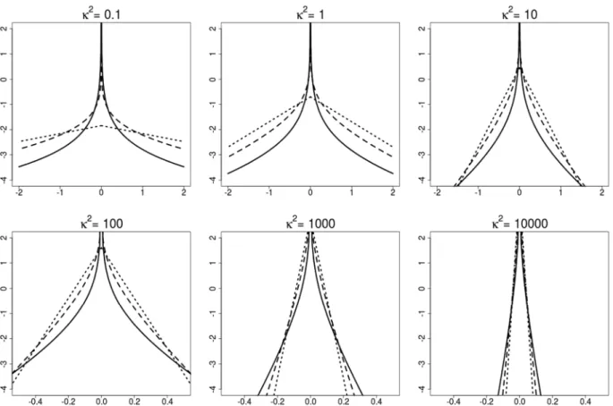
κ

2_{inFig. 1shows that the double gamma prior witha}ξ

≤

_{1 is an example of a global–local shrinkage prior (Polson}

and Scott,2011). A pronounced spike at zero is present and the mass placed close to zero strongly depends on the global

parameter

κ

2_{. From representation(13)we obtain that, marginally, E(}

θ

j)

=

2

/κ

2, whereas V(

θ

j)

=

E(

θ

j2)

−

E(

θ

j)2

=

3E((

ξ

j2) 2₎

−

4

κ

4

=

12 aξ

κ

4

+

8

κ

4

=

E(

θ

j) 2₍₂

+

₃

/

_aξ₎

.

Hence, independently ofaξ, the hyperparameter

κ

2controls the global level of shrinkage, which is the stronger, the larger

κ

2_{. At the same time, also V(}

θ

j) decreases, as

κ

increases. Therefore, the larger

κ

2, the more mass is placed close to zero. On

the other hand, the term 3

/

aξ– which is equal to the excess kurtosis of

√

θ

_j– controls local adaption to the global level of

2 _{We use the parameterization of theG(α, β)distribution with pdf given byf(y)=β}α_yα−1_e−βy_/Γ(α). 3 _{Note thatF} θj(c) = Pr(θj ≤ c) = Pr(− √ c ≤ √θj ≤ √ c) = 2F√ θj( √

c), whereFθj(·) is the cdf of the random variable √ θj. Therefore, p(θj|aξ, κ2)=p( √ θj|aξ, κ2)/ √ θj.

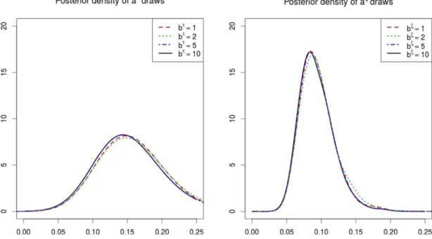
Fig. 1.Logp(√θj|aξ, κ2) of the double gamma prior for different values ofκ2andaξ=0.1 (solid line),aξ=1/3 (dashed line) andaξ=1 (dotted line).

shrinkage, with more local adaption, the smalleraξ. Asaξ decreases, the excess kurtosis of

√

θ

jincreases and the tails of

p(

√

θ

j

|

aξ

, κ

2) become thicker.

It is also illuminating to investigate the joint marginal prior distribution of (

θ

1

, . . . , θ

d) or (equivalently) of (

√

θ

1

, . . . ,

√

θ

d)

givenaξand

κ

2. Since the random prior variances

ξ

_j2in(13)are drawn independently, also marginally the double gamma

prior is characterized by prior conditional independence of (

θ

1

, . . . , θ

d) given fixed values ofaξand

κ

2:p(

θ

1

, . . . , θ

d

|

aξ

, κ

2)

=

∏

d

j=1p(

θ

j

|

aξ

, κ

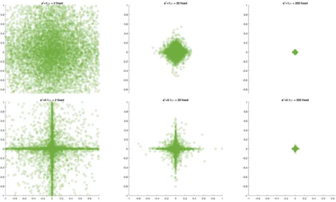
2).

For illustration,Fig. 2shows simulations from the joint priorp(

√

θ

1

,

√

θ

2

|

aξ

, κ

2) ford

=

2 for various values ofaξand

κ

2.

Not surprisingly from the previous discussions, for the same value of

κ

2_{, the double gamma witha}ξ

=

₀

.

_{1 has a pronounced}

spike at 0 with fat tails in both directions of

√

θ

1and

√

θ

2and provides more flexible shrinkage compared to the Bayesian

Lasso prior (aξ

=

1). For the Bayesian Lasso prior, large values of

κ

2_(e.g.

κ

2

=

_{200) are needed to introduce strong shrinkage}

toward 0.

To infer appropriate values ofaξ and

κ

2_{from the data, hierarchical priors are employed. We assume that}

κ

2_{follows a}

gamma distribution with fixed hyperparametersd1andd2:

κ

2

∼

_G

(

_d

1

,

d2

) .

(15)

Foraξ

=

1 this corresponds to the hierarchical Bayesian Lasso prior considered byBelmonte et al.(2014). In addition, we

assume that the shrinkage parameteraξfollows an exponential distribution as inGriffin and Brown(2010),

aξ

∼

E(bξ)

,

(16)

with a fixed hyperparameterbξ

≥

1. Combining(13)with(15)and(16)defines the hierarchical double gamma prior.

Given the hyperparametersd1,d2, andbξ, this hierarchical prior introduces prior dependence among (

θ

1

, . . . , θ

d) which

is advantageous in a shrinkage framework, as recently shown byGriffin and Brown(2017). Prior dependence is desirable in

situations, where only a few variances are expected to be different from 0. In this case, whether a certain process variance is shrunken toward 0 depends on how close the other process variances are to 0.

Prior dependence also exists between

β

j0 and

θ

j, as the size (but not the sign) of

β

j0

−

β

j depends on

θ

j through

V(

β

j0

−

β

j

|

θ

j)

=

θ

jP0,jj. If

θ

jis shrunken toward 0, then

β

j0and all subsequent values

β

jtare pulled toward

β

jfor covariatextj. In

Fig. 2. Simulations from the double gamma priorp(

√

θ1,

√

θ2|aξ, κ2) foraξ =1 (top) andaξ =0.1 (bottom) for different values ofκ2(left-hand side: κ2_{=2, middle:κ}2_{=20, right-hand side:κ}2_{=200). The plots at the top correspond to the Bayesian Lasso prior.}

β

jtto be insignificant throughout the entire observation period. As these coefficients are characterized by a parameter setting

where both

θ

jand

β

jare close to 0, a second normal–gamma prior is employed as a shrinkage prior for

β

jto allow shrinkage

of

β

jtoward 04:

β

j

|

τ

j2

∼

N

(

0

, τ

_j2

)

,

τ

2 j

|

aτ

, λ

2

∼

_G

(

aτ

,

aτ

λ

2

/

2

)

.

(17)

In this case, any (practically constant) coefficient

β

jtis insignificant, whenever the corresponding fixed regression effect

β

j

is zero.5Similarly as for

θ

j, another layer of hierarchy is added, by assuming that

λ

2

∼

G

(

e1

,

e2

)

andaτ

∼

E(bτ) with fixed

hyperparameterse1

,

e2andbτ

≥

1.

3. MCMC estimation

To carry out Bayesian inference for a sparse TVP model under the shrinkage priors introduced in Section2, we develop

an efficient scheme for Markov chain Monte Carlo (MCMC) sampling, given all hyperparameters, i.e.e1

,

e2

,

bτ

,

d1

,

d2

,

bξ

in the priors for

β

andQ,cP

, ν

P in the prior ofP0,11

, . . . ,

P0,dd, as well asc0

,

g0

,

G0for homoscedastic variances

σ

2 and

b_µ

,

B_µ

,

a0

,

b0

,

Bσ for parameters of the SV model(5). Bayesian inference operates in the latent variable formulation of

the TVP model and relies on data augmentation of the latent processes

β

=

(

β

₀

,

β

₁

, . . . ,

β

_T) for the centered and

β

˜

=

(

β

˜

₀

,

β

˜

₁

, . . . ,

β

˜

_T) for the non-centered parameterization. For the SV model, the log volatilitiesh

=

(h0

, . . . ,

hT) are introduced

as additional latent variables.

For the centered parameterization under the common inverted gamma prior(10)for the process variances

θ

j, Gibbs

sampling is totally standard, see e.g.Petris et al.(2009). However, if some of the process variances are small, then this MCMC

scheme suffers from slow convergence and poor mixing of the sampler. As shown byFrühwirth-Schnatter and Wagner

(2010), MCMC estimation based on the non-centered parameterization proves to be useful, in particular if process variances

are close to 0.

Frühwirth-Schnatter(2004) discusses the relationship between the various parametrizations for a simple TVP model and

the computational efficiency of the resulting MCMC samplers, see alsoPapaspiliopoulos et al.(2007). For TVP models with

4 _{A closed form expression, comparable to(14), is available forp(β}

j|aτ, λ2), with expectation E(|βj|)=

√ 4

πaτλ2Γ (aτ+1/2)

Γ(aτ) , V(βj)=_λ22, while the excess kurtosis is given by 3

aτ.

5 _{It should be noted that the data are not informative aboutβ}

j, ifθj>0, but they are always informative about the initial regression coefficientβj0. For θj=0,βj0andβjcoincide.

d

>

1, MCMC estimation in the centered parameterization is preferable for all coefficients that are actually time-varying, whereas the non-centered parameterization is preferable for (nearly) constant coefficients. For practical time series analysis, both types of coefficients are likely to be present and choosing a computationally efficient parameterization in advance is not possible.

We show how these two data augmentation schemes can be combined through theancillarity-sufficiency interweaving

strategy(ASIS) introduced byYu and Meng(2011) to obtain an efficient sampler combining the ‘‘best of both worlds’’. ASIS provides a principled way of interweaving different data augmentation schemes by re-sampling certain parameters conditional on the latent variables in the alternative parameterization of the model. This strategy has been successfully

employed to univariate SV models (Kastner and Frühwirth-Schnatter,2014), multivariate factor SV models (Kastner et al.,

2017) and dynamic linear state space models (Simpson et al.,2017). In the present paper, ASIS is applied to interweave the

centered and the non-centered parameterization of a TVP model. More specifically, we use the non-centered parameteriza-tion as baseline, and interweave into the centered parameterizaparameteriza-tion. This leads to the MCMC sampling scheme outlined in

Algorithm 1which increases posterior sampling efficiency considerably compared to conventional Gibbs sampling for either of the two parameterizations.

Algorithm 1. Choose starting values for

β

,

Q,

τ

=

(

τ

1

, . . . , τ

d),

ξ

=

(

ξ

1

, . . . , ξ

d),aτ

, λ

2

,

aξ,

κ

2

,

P0, and (for homoscedastic

variances)

σ

2_andC

0and repeat the following steps:

(a) Sample the states

β

˜

=

(

β

˜

₀

, . . . ,

β

˜

_T) in the non-centered parameterization from the multivariate Gaussian posterior

˜

β

|

β

,

Q

,

P0

, σ

2

∼

N(T+1)d

(

Ω−1c

,

Ω−1

)

given in (A.1). (b) Joint sampling of

α

=

(

β

1

, . . . , β

d

,

√

θ

1

, . . . ,

√

θ

d)′from the multivariate Gaussian posteriorp(

α

| ˜

β

,

τ

,

ξ

, σ

2

,

y) given

in (A.3).

(c) For eachj

=

1

, . . . ,

d, redraw the constant coefficient

β

jand the square root of the process variance

√

θ

jthrough

interweaving into the state equation of the centered parameterization:

(c-1) Use the transformation(8)to match the draws of the latent process

β

˜

j0

, . . . ,

β

˜

jT in the non-centered to the

latent process

β

j0

, . . . , β

jTin the centered parameterization and store the sign of

√

θ

j.

(c-2) Update

β

jand

θ

jin the centered parameterization by sampling

θ

jnewfrom the generalized inverse Gaussian

posterior

θ

j

|

β

j0

, . . . , β

jT

, β

j

, ξ

j2

,

P0,jj, given in(18), and

β

jnewfrom the Gaussian posterior

β

j

|

β

j0

, θ

jnew

, τ

j2

,

P0,jj,

given in(19).

(c-3) Determine

√

θ

new

j using the same sign as the old value

√

θ

j. Based on

√

θ

new

j and

β

jnew, the state process

β

˜

jtin the

non-centered parameterization is updated in a deterministic manner through the inverse of the transformation

(8):

˜

β

jtnew

=

(

β

jt

−

β

newj )

/

√

θ

new j

,

t

=

0

, . . . ,

T

.

(d) Sample fromaτ

|

β

1

, . . . , β

d

, λ

2andaξ

|

√

θ

1

, . . . ,

√

θ

d

, κ

2using a random walk Metropolis–Hastings (MH) step based

on proposing logaτ,new

∼

_N

(

logaτ

,

c2

τ

)

and logaξ,new

∼

N

(

logaξ

,

cξ2

)

.

(e) Sample the prior variances

τ

j

|

β

j

,

aτ

, λ

2and

ξ

j

|

θ

j

,

aξ

, κ

2, forj

=

1

, . . . ,

d, from conditionally independent generalized

inverse Gaussian distributions given in (A.4) and (A.5), respectively, and update the hyperparameters

λ

2

|

_aτ

,

τ

_and

κ

2

|

_aξ

,

ξ

_{from the gamma distributions given in (A.6) and (A.7).}

(f) Sample

σ

2

| ˜

β

,

α

,

_C

0

,

yfrom the following inverted gamma distribution

σ

2

| ˜

β

,

α

,

_C 0

,

y

∼

G −1

(

c0

+

T 2

,

C0

+

1 2 T

∑

t=1 (yt

−

zt

α

)2

)

,

whereztis defined in (A.2), and sampleC0fromC0

|

σ

2

∼

G

(

g0

+

c0

,

G0

+

_σ12

)

.

(g) Sample the scale parameters of the initial distribution for eachj

=

1

, . . . ,

d, fromP0,jj

| ˜

β

j0

∼

G−1

(

ν

P

+

1₂

,

(

ν

P

−

1)cP

+

1 2

β

˜

2 j0

)

.

After discarding a certain amount of initial draws (theburn-in), the full conditional sampler iterating Steps (a) to (g) of

Al-gorithm 1yields draws from the joint posterior distributionp(

β

˜

, β

1

, . . . , β

d

,

√

θ

1

, . . . ,

√

θ

d

,

τ

,

ξ

,

aτ

, λ

2

,

aξ

, κ

2

,

P0

, σ

2

,

C0

,

|

y)

under the hierarchical shrinkage priors outlined in Section2.2.

In Step (a), we sample the latent states

β

˜

=

(

β

˜

₀

, . . . ,

β

˜

_T) in the non-centered parameterization conditional on known

parameters

β

,

Q

,

P0and known error variances

σ

2. As an alternative to the commonly usedForward Filtering Backward

Sampling(Frühwirth-Schnatter,1994;Carter and Kohn,1994), we implemented a multi-move sampling algorithm in the

spirit ofMcCausland et al.(2011) which allows to sample the entire state process

β

˜

all without a loop(AWOL;Kastner and

Frühwirth-Schnatter(2014)). Full details are provided in Appendix A.1.1.1.

In Step (b), conditional on the latent states

β

˜

, a regression type model results from the observation equation(9)of

shrinkage priors(12)and(17), we sample the parameters

β

1

, . . . , β

d and

√

θ

1

, . . . ,

√

θ

d jointly from the conditionally

Gaussian posterior given in (A.3); see Appendix A.1.1.2 for details. One major advantage of working with the square root

of the process variance

√

θ

j, instead of

θ

j, is that we avoid boundary space problems for small variances, resulting in better

mixing behavior of the sampler.

The interweaving Step (c) turns out to be instrumental for an efficient implementation of the hierarchical shrinkage

priors introduced in Section2.2. In this step, we temporarily move from the non-centered to the centered parameterization

to resample

β

jand

θ

j. To ensure that the posterior distributions obtained with and without interweaving are identical, the

priors between the non-centered and the centered parameterization are matched. Whereas the Gaussian prior

β

j

|

τ

j2for the

initial value

β

jis the same for both parameterizations, we transform the Gaussian prior for

√

θ

j

|

ξ

j2to the corresponding

gamma prior for

θ

j

|

ξ

j2in the centered parameterization, see(11). In Step (c-2), the posteriors of

θ

jand

β

jin the centered

parameterization, conditional on the state process

β

j0

, . . . , β

jT, are easily obtained. First, the conditional posterior

p(

θ

j

|

β

j0

, . . . , β

jT

, β

j

, ξ

j2

,

P0,jj)

∝

p(

θ

j

|

ξ

j2)p(

β

j0

|

β

j

, θ

j

,

P0,jj) T

∏

t=1 p(

β

jt

|

β

j,t−1

, θ

j)

,

where

β

j0

|

β

j

, θ

j

,

P0,jj

∼

N

(

β

j

, θ

jP0,jj

)

and

β

jt

|

β

j,t−1

, θ

j

∼

N

(

β

j,t−1

, θ

j

)

, is the density of a generalized inverse Gaussian distribution (GIG) with following parameters:

θ

j

|

β

j0

, . . . , β

jT

, β

j

, ξ

j2

,

P0,jj

∼

GIG

(

−

T 2

,

1

ξ

2 j

,

T

∑

t=1 (

β

jt

−

β

j,t−1)2

+

(

β

j0

−

β

j)2 P0,jj

)

.

(18)

Note that sampling the process variance

θ

j from this GIG posterior6 deviates from the usual MCMC inference for the

centered state space model, since the conditionally conjugate inverted gamma prior(10)is substituted by a prior from the

gamma distribution. Second, the posteriorp(

β

j

|

β

j0

, θ

j

, τ

j2

,

P0,jj) is a Gaussian distribution, obtained by combining the prior

β

j

|

τ

j2

∼

N

(

0

, τ

2

j

)

with the conditional likelihood

β

j0

|

β

j

, θ

j

,

P0,jj

∼

N

(

β

j

, θ

jP0,jj

)

:

β

j

|

β

j0

, θ

j

, τ

j2

,

P0,jj

∝

N

(

β

j0

τ

j2

τ

2 j

+

θ

jP0,jj

,

τ

2 j

θ

jP0,jj

τ

2 j

+

θ

jP0,jj

)

.

(19)

Sampling the parametersaτandaξin Step (d) is performed without conditioning on

τ

1

, . . . , τ

dand

ξ

1

, . . . , ξ

d. The acceptance

probability foraξ,new_reads:

min

{

1

,

p(a ξ,new_)aξ,new p(aξ)aξ d

∏

j=1 p(

√

θ

j

|

aξ,new

, κ

2) p(

√

θ

j

|

aξ

, κ

2)

}

,

based on the marginal prior(14). A similar acceptance probability holds foraτ,new_.

Sampling the latent prior variances

τ

2

j and

ξ

j2of the hierarchical shrinkage priors(17)and(12)for

β

jand

√

θ

jin Step (e)

is less standard and we briefly discuss sampling

ξ

2

j (full details are given in Appendix A.1.1.3). The conditionally normal

prior

√

θ

j

|

ξ

j2in(12)leads to a likelihood for

ξ

j2which is the kernel of an inverted gamma density. In combination with the

gamma prior for

ξ

2

j

|

aξ

, κ

2, this leads to a posterior distribution arising from a generalized inverse Gaussian (GIG) distribution:

ξ

2 j

|

θ

j

,

aξ

, κ

2

∼

GIG

(

aξ

−

1

/

2

,

aξ

κ

2

, θ

j

)

.

Finally, Step (f) has to be modified for the SV model defined in(5). To sample (h0

, . . . ,

hT) as well as

µ

,

φ

, and

σ

_η2, we rely

onKastner and Frühwirth-Schnatter(2014) who developed an interweaving strategy for boosting MCMC estimation of SV

models.7

4. Comparing shrinkage priors through log predictive density scores

Log predictive density scores (LPDS) are an often used scoring rule to compare models; see, e.g.,Gneiting and Raftery

(2007).Geweke and Keane(2007) introduced LPDS for model comparison of econometric models, see alsoGeweke and Amisano(2010) for an excellent review of Bayesian predictive analysis. In the present paper, we use log predictive density scores as a means of evaluating and comparing different shrinkage priors.

As common in this framework, the firstt0time series observationsytr

=

(y1

, . . . ,

yt0) are used as a ‘‘training sample’’,

while evaluation is performed for the remaining time series observationsyt0+1

, . . . ,

yT, based on the log predictive density:

LPDS

=

logp(yt0+1

, . . . ,

yT

|

y tr₎

=

T

∑

t=t0+1 logp(yt

|

yt−1)

=

T

∑

t=t0+1 LPDS⋆_t

.

(20)

6 _{To sample from the GIG distribution, we use a method proposed byHörmann and Leydold(2014) which is implemented in the R-package}

GIGrvg(Hörmann and Leydold,2015). This method is especially reliable for TVP models where the scale parameters of the GIG distribution can be extremely small due to shrinkage and other samplers tend to fail.

In(20),p(yt

|

yt−1) is the one-step ahead predictive density for timetgivenyt−1

=

(y1

, . . . ,

yt−1) which is evaluated at the

observed valueyt. The (individual) log predictive density scores LPDS⋆t

=

logp(yt

|

yt−1) provide a tool to analyze performance

separately for each observationyt, whereas LPDS is an aggregated measure of performance for the entire time series.

As shown byFrühwirth-Schnatter(1995) in the context of selecting time-varying and fixed components for a basic

structural state space model, LPDS can be interpreted as a log marginal likelihood based on the training sample priorp(

ϑ

|

ytr_),

since p(yt0+1

, . . . ,

yT

|

y tr₎

=

∫

p(yt0+1

, . . . ,

yT

|

y tr

,

ϑ

_)p(

ϑ

|

_ytr_)d

ϑ

,

where

ϑ

summarizes the unknown model parameters, e.g.

ϑ

=

(

β

1

, . . . , β

d,

√

θ

1

, . . . ,

√

θ

d

, σ

2) for the homoscedastic state

space model. This provides a sound and coherent foundation for using the log predictive density score for model – or, in our context, rather prior – comparison.

To approximate the one-step ahead predictive densityp(yt

|

yt−1), we use Gaussian sum approximations, which are derived

from the MCMC draws (

ϑ

(m)

,

m

=

1

, . . . ,

M) from the posterior distributionp(

ϑ

|

yt−1_{) given information up toy}t−1_{, i.e:}

LPDS∗_t

=

logp(yt

|

yt −1₎

=

_log

∫

p(yt

|

yt −1

,

ϑ

_)p(

ϑ

|

_yt−1_)d

ϑ

≈

_log

(

1 M M

∑

m=1 p(yt

|

yt −1

,

ϑ

(m)₎

)

,

(21)

where the one-step ahead predictive densityp(yt

|

yt−1

,

ϑ

) is Gaussian conditional on knowing

ϑ

.

We derive an approximation, called theconditionally optimal Kalman mixture approximation, which exploits the fact that

the TVP model is a conditionally Gaussian state space model given

ϑ

=

(

β

1

, . . . , β

d

,

√

θ

1

, . . . ,

√

θ

d

, σ

t2).8For each draw

ϑ

(m)

=

₍

β

(m) 1

, . . . , β

(m) d ,

√

θ

1 (m)

, . . . ,

√

θ

d (m)

,

σ

_t2(m)) from the posteriorp(

ϑ

|

yt_{), we determine theexactpredictive density}

p(yt

|

yt−1

,

ϑ

(m)) given by the normal distributionyt

|

yt−1

,

ϑ

(m)

∼

Nd

(

ˆ

y(_tm)

,

S_t(m)

)

, wherey

ˆ

(_tm)andS_t(m)are obtained from the

prediction step of the Kalman filter (see Appendix A.1.2.1), based on the filtering density

β

˜

_t−1

|

yt

−1

,

ϑ

(m)

∼

_N d

(

m(_tm−)1

,

C (m) t−1

)

:

ˆ

y(_tm)

=

xt

β

(m)

+

F(tm)m (m) t−1

,

S_t(m)

=

F(_tm)(C(_tm−)1

+

Id)F ′(m) t

+

σ

2(m) t

,

whereF(_tm)

=

x_tDiag

(

√

θ

1 (m)

, . . . ,

√

θ

d (m)

)

andI_dis thed

×

didentity matrix. This yields the following Gaussian mixture

approximation forp(yt

|

yt−1): p(yt

|

yt −1₎

≈

1 M M

∑

m=1 fN

(

yt

; ˆ

y(tm)

,

S (m) t

)

.

(22)

Draws fromp(

ϑ

|

yt−1) are obtained by running the Gibbs sampler outlined inAlgorithm 1for the reduced sampleyt−1

=

(y1

,

y2

, . . . ,

yt−1). For a homoscedastic error specification,

σ

t2(m)

≡

σ

2(m), whereas

σ

2(m)

t is forecasted in the following way

for the SV model(5). Given the posterior drawh(_tm−)1, we simulateh

(m)

t from a conditional normal distribution with mean

µ

(m)

+

φ

(m)_(h(m)

t−1

−

µ

(m)) and variance

σ

η2(m)and define

σ

2(m)

t

=

eh (m) t _.

5. Extension to multivariate time series 5.1. Sparse TVP models for multivariate time series

The methods introduced in the previous sections are easily extended to TVP models for multivariate time series, such as

time-varying parameter VARs, see e.g.Eisenstat et al.(2014) who analyze the response of macro variables to fiscal shocks,

and time-varying structural VARs, see e.g.Primiceri(2005) for a monetary policy application. Consider, as illustration, the

following TVP model for anr-dimensional time seriesy_t,

yt

=

Btxt

+

ε

t

,

ε

t

∼

Nr

(

0

,

Σt

) ,

(23)

wherextis acolumnvector ofdregressors, andBtis a time-varying (r

×

d) matrix with coefficient

β

ij,tin rowiand columnj,

potentially containing structural zeros or constant values such that

β

ij,t

≡

capriori. The (apriori) unconstrained time-varying

coefficients

β

ij,tare assumed to follow independent random walks as in the univariate case:

β

ij,t

=

β

ij,t−1

+

ω

ij,t

, ω

ij,t

∼

N

(

0

, θ

ij

)

,

(24)

with initial value

β

ij,0

∼

N

(

β

ij

, θ

ijP0,ijj

)

, whereP0,ijj

∼

G−1

(ν

P

,

(

ν

P

−

1)cP

)

as before. Both the fixed regression coefficients

β

ijas well as the process variances

θ

ijare assumed to be unknown.

Each of the apriori unconstrained coefficients

β

ij,t is potentially constant, with the corresponding process variance

θ

ij

being 0. A constant coefficient

β

ij,t

≡

β

ij is potentially insignificant, in which case

β

ij

=

0. Hence, shrinkage priors as

introduced in Section2.2for the univariate case, are imposed on the

θ

ijs and

β

ijs to define a sparse TVP model for identifying

which of these scenarios holds for each coefficient

β

ij,t.

Fori

=

1

, . . . ,

r, the hierarchical double gamma prior for the process variances

θ

ijof the coefficients in theith row of a

multivariate TVP model reads:

θ

ij

|

ξ

ij2

∼

G

(

1 2

,

1 2

ξ

2 ij

)

, ξ

2 ij

|

aξi

, κ

2 i

∼

G

(

aξ_i

,

aξ_i

κ

_i2

/

2

)

, κ

2 i

∼

G

(

d1

,

d2

) ,

aξ_i

∼

E(bξ)

,

(25)

with prior expectation

ξ

2

ijfor each process variance

θ

ij. Similarly, an individual prior variance

τ

ij2is introduced for each fixed

regression coefficient

β

ijas in(17):

β

ij

|

τ

ij2

∼

N

(

0

, τ

_ij2

)

, τ

2 ij

|

aτi

, λ

2 i

∼

G

(

aτ_i

,

aτ_i

λ

2_i

/

2

)

, λ

2 i

∼

G

(

e1

,

e2

) ,

aτi

∼

E(bτ)

.

(26)

By choosingaτ_i

=

aξ_i

=

1 in(25)and(26), a hierarchical Bayesian Lasso prior for multivariate TVP models results.

We assume row specific hyperparametersaτ_i

, λ

2_i andaξ_i

, κ

_i2, drawn from common hyperpriors with fixed

hyperparam-eterse1

,

e2

,

bτ andd1

,

d2

,

bξ. This leads to prior independence across ther rows of the observation equation(23)and is

advantageous for computational reasons, in particular, if the errors

ε

t are uncorrelated, i.e.Σt is a diagonal matrix. In

this case, the multivariate TVP model has a representation asr independent univariate TVP models as in Section2.1and

MCMC estimation usingAlgorithm 1can be performed independently for each of therrows of the system, e.g. in a parallel

computing environment.

IfΣt is a full covariance matrix, then the rows are not independent, because of the correlation among the various

components in

ε

t. However, as shown byLopes et al.(2016), a Cholesky decomposition ofΣtleads to such a representation,

see alsoEisenstat et al.(2014) andZhao et al.(2016). Further details are provided in the next subsection.

5.2. The sparse TVP Cholesky SV model

Lopes et al.(2016) demonstrate how a multivariate time seriesyt

∼

Nr

(

0

,

Σt

)

with time-varying covariance matrixΣt

can be transformed into a system ofrindependent equations using the time-varying Cholesky decompositionΣt

=

AtDtA′t

, whereA_tD1_t/2is the lower triangular Cholesky decomposition ofΣt.Atis lower triangular with ones on the main diagonal,

whileD_tis a time-varying diagonal matrix. It follows thatA−1_t y_t

∼

N_r

(

0

,

D_t

)

. Denoting the elements ofA−1_t asΦij,t, forj

<

i,

this can be expressed as

⎛

⎜

⎜

⎜

⎜

⎜

⎝

1

. . .

0 Φ21,t 1 0

...

0

...

1 0 Φr1,t Φr2,t

. . .

Φr,r−1,t 1

⎞

⎟

⎟

⎟

⎟

⎟

⎠

⎛

⎜

⎜

⎝

y1t y2t

...

yrt

⎞

⎟

⎟

⎠

∼

Nr

(

0

,

Dt

) ,

which can be written as in(23):

yt

∼

Nr

(

Btxt

,

Dt

) ,

(27)

whereB_tis ar

×

(r

−

1) matrix with elements

β

ij,t

= −

Φij,t,Dt is a diagonal matrix and the (r

−

1)-dimensional vector

xt

=

(y1t

, . . . ,

yr−1,t)′ is a regressor derived fromyt. Thus the distribution ofyt can be represented by a system ofr

independent TVP models as in Section5.1, where each time-varying coefficient

β

ij,t

,

j

<

i,i

=

1

, . . . ,

r, follows a random

walk as in(24). Employing the prior(26)for

β

ijand(25)for

θ

ijyields the sparse TVP Cholesky SV model.

To capture conditional heteroscedasticity, the matrixDt

=

Diag

(

eh1t

, . . . ,

_ehrt

)

_{is assumed to be time-varying, where for}

each rowi

=

1

, . . . ,

r, the log volatilityhitis assumed to follow an individual SV model as in(5), with row specific parameters

µ

i,

φ

i, and

σ

_η,2i: hit

|

hi,t−1

, µ

i

, φ

i

, σ

_η,2i

∼

N

(

µ

i

+

φ

i(hi,t−1

−

µ

i)

, σ

_η,2i

)

.

Forr

=

3, for instance, the TVP Cholesky SV model reads:

y1t

=

ε

1t

,

ε

1t

∼

N

(

0

,

eh1t

)

,

y2t

=

β

21,ty1t

+

ε

2t

,

ε

2t

∼

N

(

0

,

eh2t

)

,

y3t

=

β

31,ty1t

+

β

32,ty2t

+

ε

3t

,

ε

3t

∼

N

(

0

,

eh3t

)

.

Table 1

Simulated data. Average mean squared error (avMSE), average variance (avVAR), and average squared bias (avBIAS2_{) over} 100 simulated time series for the hierarchical double gamma prior withaτ ∼E(10) andaξ ∼E(10) and the hierarchical Bayesian Lasso prior withaτ=aξ=1.

aτ ∼E(10),aξ∼E(10) aτ =aξ=1

avMSE avVAR avBIAS2 _{avMSE avVAR avBIAS}2

β1 3.30E−01 1.67E−01 1.63E−01 3.60E−01 1.57E−01 2.03E−01

β2 8.18E−03 8.11E−03 6.47E−05 1.56E−02 1.55E−02 1.77E−04

β3 2.10E−03 2.10E−03 1.36E−06 1.14E−02 1.13E−02 1.31E−04

|√θ1| 1.81E−03 1.79E−03 2.50E−05 1.61E−03 1.56E−03 5.32E−05

|√θ2| 1.14E−04 9.33E−05 2.11E−05 5.02E−04 2.47E−04 2.55E−04

|√θ3| 4.33E−05 3.53E−05 7.97E−06 3.10E−04 1.44E−04 1.66E−04

No intercept is present in these TVP models. For the TVP model in the first row, no regressors are present and only the

time-varying volatilitiesh1t have to be estimated. In theith equation,i

−

1 regressors are present andd

=

i

−

1

time-varying regression coefficients

β

ij,tas well as the time-varying volatilitieshitneed to be estimated. Each of these equations

is transformed into a non-centered TVP model and the MCMC scheme inAlgorithm 1is applied to perform Bayesian inference

independently for each rowi.

6. Illustrative application to simulated data

To illustrate our methodology for simulated data, we generated 100 univariate time series of lengthT

=

200 from

a TVP model whered

=

3,

{

x1t

} ≡

1,

{

xjt

} ∼

N

(

0

,

1

)

for j

=

2

,

3,

σ

2

=

1, (

β

1

, β

2

, β

3)

=

(1

.

5

,

−

0

.

3

,

0) and

(

θ

1

, θ

2

, θ

3)

=

(0

.

02

,

0

,

0). For each time series,

β

1t is a strongly time-varying coefficient,

β

2t is a constant, but significant

coefficient, and

β

3t is an insignificant coefficient. As shrinkage priors on

β

jand

√

θ

j, we consider the hierarchical double

gamma prior withaτ

∼

E(10) andaξ

∼

E(10) and the hierarchical Bayesian Lasso prior (that isaτ

=

aξ

=

1) under the

hyperparameter settingd1

=

d2

=

e1

=

e2

=

0

.

001. For each of the 100 simulated time series, MCMC estimation is based

onAlgorithm 1by drawingM

=

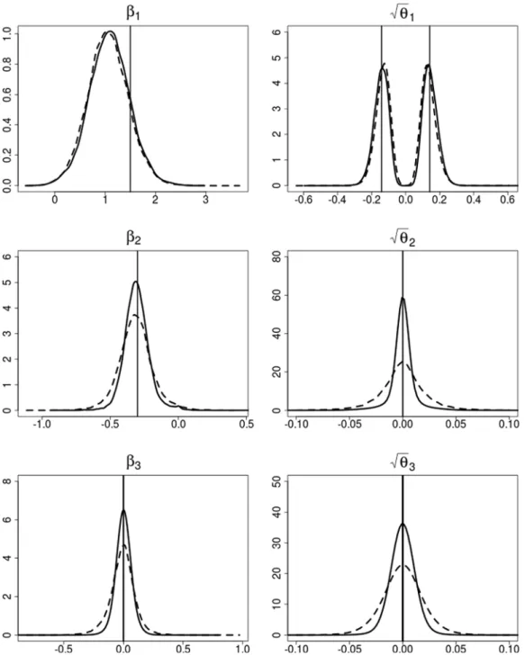
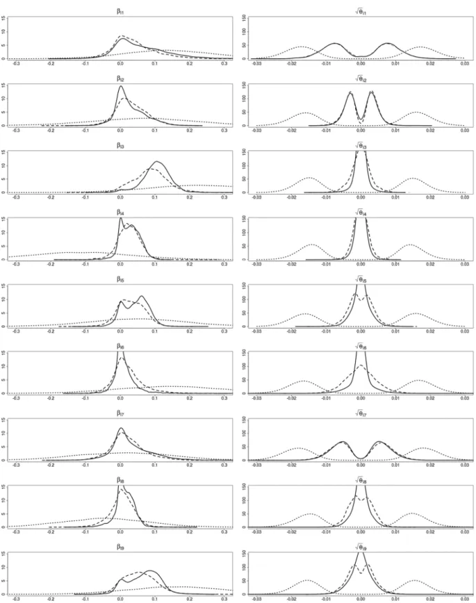
30,000 samples after a burn-in of length 30,000.9 InFig. 3we compare the posterior densities for

β

jand

√

θ

jfor one such time series under both shrinkage priors. In general,

we want to distinguish three types of coefficients: time-varying, static but significant, and insignificant. One way to achieve a

classification is by visual inspection of the posterior distributions of

β

jand

√

θ

j. The posterior density of the scale parameter

√

θ

jis symmetric around zero by definition. Thus, if the unknown variance

θ

jis different from zero, then the posterior density

of

√

θ

jis likely to be bimodal. If we find that the posterior density of

√

θ

jis unimodal, then the unknown variance is likely

to be zero.

While such a bimodal structure ofp(

√

θ

j

|

y) is well pronounced for the first coefficient where

√

θ

1

=

0

.

141,p(

√

θ

j

|

y) is

indeed shrunken toward zero for the two coefficients with zero variances

θ

2

=

θ

3

=

0. For the third coefficient, where in

addition

β

3

=

0, also the posteriorp(

β

3

|

y) is shrunken toward zero. Further, we show the posterior paths of

β

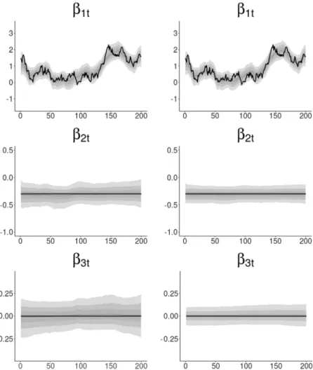
jtin Fig. 4.

Evidently, shrinkage priors are able to detect the time-varying coefficient

β

1t, the constant but significant coefficient

β

2tand

the insignificant coefficient

β

3t. In both figures, the advantage of the double gamma prior compared to the Bayesian Lasso

prior is reflected by increased efficiency in identifying coefficients that are not time-varying.

Table 1summarizes the average mean squared error (a

v

MSE), the average squared bias (a

v

BIAS2_{) and the average variance}

(a

v

VAR) for the parameters

β

1,

β

2,

β

3,

|

√

θ

1

|

,

|

√

θ

2

|

, and

|

√

θ

3

|

over the 100 simulated time series.10Heavier shrinkage

introduced by the hierarchical double gamma prior leads to reduceda

v

MSEcompared to the hierarchical Bayesian Lasso

prior, in particular for the two coefficients which are not time-varying.

7. Applications in economics and finance 7.1. Modeling EU area inflation

As a first application, we reconsider EU-area inflation data analyzed inBelmonte et al.(2014) and consider the generalized

Phillips curve specification, where inflation

π

tdepends on (typicallyp

=

12) lags of inflation and other predictorszt:

π

t+h

=

p−1

∑

j=0

φ

jt

π

t−j

+

zt

γ

t

+

ε

t+h

, ε

t+h

∼

N

(

0

, σ

2

)

.

(28)

9 _{The Bayesian Lasso prior is combined with the ASIS strategy by fixinga}τ _=aξ_{=1 and skipping Step (d).}

10 _{GivenMdrawsϑ}(i1)_{, . . . , ϑ}(iM)_{, of a parameterϑfor each time seriesi, these measures are defined asavMSE=avVAR+avBIAS}2_{, whereavVAR=} 1

100 ∑100

i=1ViandavBIAS2=₁₀₀1 ∑100i=1(Ei−ϑtrue)2with Ei=_M1 ∑Mm=1ϑ (im)_{and V}

i=_M1 ∑Mm=1(ϑ (im)_−E

Fig. 3. Simulated data. Posterior densities ofβj(left-hand side) and

√

θj(right-hand side) together with the true values (indicated by the vertical lines),

based on the hierarchical double gamma prior withaτ∼E(10) andaξ∼E(10) (solid line) and the hierarchical Bayesian Lasso prior (dashed line).

This set-up has been discussed byStock and Watson(2012), among others, for forecasting the annual inflation rate, that is

h

=

12. Data are monthly and range from February 1994 until November 2010, i.e.T

=

190. We list precise definitions

of all variables in Appendix A.2.1. As the time series are not seasonally adjusted, we include monthly dummy variables as

covariates in(28)to account for seasonal patterns. Thus we are estimating in totald

=

37 possibly time-varying coefficients,

consisting of the intercept, 13 regressors like theunemployment rateand the1-month interest rate, 12 lagged values of

inflation and 11 seasonal dummies.

As shrinkage priors on

β

jand

√

θ

j, we consider the hierarchical double gamma prior withaτ

∼

E(bτ) andaξ

∼

E(bξ) under

the hyperparameter settingd1

=

d2

=

e1

=

e2

=

0

.

001 and compare it with the hierarchical Bayesian Lasso prior (that is

Fig. 4. Simulated data. Pointwise (0.025,0.25,0.5,0.75,0.975)-quantiles of the posterior pathsβjt =βj+

√

θjβ˜jtin the centered parameterization in

comparison to the true paths (thick black line) for one of the simulated time series; left-hand side: hierarchical Bayesian Lasso prior, right-hand side: hierarchical double gamma prior withaτ∼E(10) andaξ∼E(10).

Table 2

ECB data. Posterior summaries forp(aτ|y) andp(aξ|y) for various valuesbτ=bξ.

bτ =bξ p(aτ|y) p(aξ|y)

1st Qu. Median Mean 3rd Qu. 1st Qu. Median Mean 3rd Qu.

1 0.128 0.153 0.158 0.181 0.078 0.091 0.094 0.107

2 0.127 0.151 0.158 0.181 0.078 0.092 0.096 0.109

5 0.124 0.147 0.153 0.174 0.076 0.090 0.094 0.107

10 0.122 0.145 0.150 0.172 0.074 0.088 0.090 0.103

draws after a burn-in of the same size. For the hierarchical double gamma prior, we considered various hyperparametersbτ

andbξand the corresponding posterior densities ofaτ andaξare shown inFig. 5, with posterior summaries being provided

inTable 2. The acceptance probability for the random walk MH algorithm in Step (d) ofAlgorithm 1lies in the range of 0.24

to 0.26. For these data, the posteriors ofaτ andaξ clearly point at the double gamma prior rather than the Bayesian Lasso

prior. The choice of the hyperparametersbτandbξdoes not play a significant role and the following results are presented

forbτ

=

bξ

=

10.

Summary statistics ofp(

β

j

|

y) andp(

√

θ

j

|

y) for the hierarchical double gamma prior withaτ

∼

E(10) andaξ

∼

E(10)

are given in Table A.3 in Appendix A.3.1. The easiest combination to spot is the case where both parameters

β

jand

√

θ

jare

shrunken toward zero and the corresponding posterior densities exhibit peaks at zero. This is the case for most of the 37

covariates. The posterior median of

√

|

θ

_j

|

in Table A.3 is smaller than 10−3_{for 34 regression coefficients, among them the}

lagged values of inflation and the monthly dummy variables. In addition, for these coefficients the 95%-confidence regions

Fig. 5. ECB data. Posterior density ofaτ(left-hand side) andaξ(right-hand side).

Table 3

ECB data. Inefficiency factors of MCMC posterior draws of selected parameters, obtained fromAlgorithm 1with and without interweaving under the hierar