Machine Learning for Personalised Medicine
Inauguraldissertation zur
Erlangung der W¨urde eines Doktors der Philosophie vorgelegt der
Philosophisch-Naturwissenschaftlichen Fakult¨at der Universit¨at Basel
von
Sonali Parbhoo
aus Johannesburg, S¨udafrika und USA 2019
Original document stored on the publication server of the University of Basel edoc.unibas.ch. This work is licensed under the agreement “Attribution Non-Commercial No Derivatives - 4.0 International”.
Genehmigt von der Philosophisch-Naturwissenschaftlichen Fakult¨at auf Antrag von
Prof. Dr. Volker Roth, Dissertationsleiter Prof. Dr. Niko Beerenwinkel, Korreferent
Basel, den 25. Juni 2019
This is a human-readable summary of (and not a substitute for) the license.
You are free to:
Share— copy and redistribute the material in any medium or format.
The licensor cannot revoke these freedoms as long as you follow the license terms.
Under the following terms:
Attribution— You must give appropriate credit, provide a link to the license, and indicate if changes were made. You may do so in any reasonable manner, but not in any way that suggests the licensor endorses you or your use.
Non-Commercial— You may not use the material for commercial purposes.
No Derivatives— If you remix, transform, or build upon the material, you may not dis-tribute the modified material.
No additional restrictions— You may not apply legal terms or technological measures that legally restrict others from doing anything the license permits.
Notices:
You do not have to comply with the license for elements of the material in the public domain or where your use is permitted by an applicable exception or limitation.
No warranties are given. The license may not give you all of the permissions necessary for your intended use. For example, other rights such as publicity, privacy, or moral rights may limit how you use the material.
In this thesis, we discuss the importance of causal knowledge in healthcare for tailoring treatments to a patient’s needs. We propose three different causal models for reason-ing about the effects of medical interventions on patients with HIV and sepsis, based on observational data. Both application areas are challenging as a result of patient heterogeneity and the existence of confounding that influences patient outcomes.
Our first contribution is a treatment policy mixture model that combines nonpara-metric, kernel-based learning with model-based reinforcement learning to reason about a series of treatments and their effects. These methods each have their own strengths: non-parametric methods can accurately predict treatment effects where there are over-lapping patient instances or where data is abundant; model-based reinforcement learn-ing generalises better in outlier situations by learnlearn-ing a belief state representation of confounding. The overall policy mixture model learns a partition of the space of het-erogeneous patients such that we can personalise treatments accordingly.
Our second contribution incorporates knowledge from kernel-based reasoning di-rectly into a reinforcement learning model by learning a combined belief state represen-tation. In doing so, we can use the model to simulate counterfactual scenarios to reason about what would happen to a patient if we intervened in a particular way and how would their specific outcomes change. As a result, we may tailor therapies according to patient-specific scenarios.
Our third contribution is a reformulation of the information bottleneck problem for learning an interpretable, low-dimensional representation of confounding for medical decision-making. The approach uses the relevance of information to perform a sufficient reduction of confounding. Based on this reduction, we learn equivalence classes among groups of patients, such that we may transfer knowledge to patients with incomplete covariate information at test time. By conditioning on the sufficient statistic we can accurately infer treatment effects on both a population and subgroup level.
Our final contribution is the development of a novel regularisation strategy that can be applied to deep machine learning models to enforce clinical interpretability. We specifically train deep time-series models such that their predictions have high accuracy while being closely modelled by small decision trees that can be audited easily by med-ical experts. Broadly, our tree-based explanations can be used to provide additional context in scenarios where reasoning about treatment effects may otherwise be diffi-cult. Importantly, each of the models we present is an attempt to bring about more understanding in medical applications to inform better decision-making overall.
Acknowledgments
I am both deeply grateful and consider myself extremely fortunate to have worked with my supervisor, Prof. Dr. Volker Roth, without whom none of the work in this thesis would have been possible. It is difficult to articulate in words how much the opportunity to work with you means to me. Thank you for providing me with what I consider to be one of the best experiences of my life. You never failed to guide and support me when I needed it, and you always asked the right questions, even if it meant I had to re-think my ideas at the time. These experiences have taught me how to become a better researcher overall. You also gave me the freedom to explore my own ideas, even if it meant collaborating with many other researchers around the world. Most of all, when I think about the kind of scientist I would like to be some day, I know I want to be just like you . . . . Thank you.
I am very thankful to Prof. Dr. Niko Beerenwinkel for reviewing my thesis as a co-referee and for providing valuable feedback during committee meetings and the Systems-X HIV-X project. I am also very grateful to Prof. Dr. Thomas Vetter for many thought-provoking discussions about research and philosophy during lab meetings and breaks. These discussions have been the source of a lot of inspiration during the final stages of my PhD.
A significant portion of the work in this thesis was performed under the guidance of Prof. Dr. Finale Doshi-Velez. Thank you for introducing me to a lot of interesting work conducted in your research group, and providing me the opportunity to understand these problems in a way that would not have been possible otherwise. I am very fortunate to have gained some experience working with you, and I am very excited about our future research together! I would also like to thank Prof. Dr. George Konidaris for introducing me to Prof. Dr. Finale Doshi-Velez, knowing that our research interests would align well.
I am especially grateful to my Masters’ research advisor, Prof. Dr. Clint Van Alten, for encouraging me to pursue a PhD in the first place, and for providing support during one of the most difficult periods of my life. You recommended applying to Prof. Volker Roth after reading some of his work, and I have not regretted my decision ever since.
Outside the computer science department, I am glad to have been part of numerous collaborations with other researchers and medical professionals. I would especially like to thank Dr. Jasmina Bogojeska for many helpful discussions on non-parametric kernel methods, and whose work has inspired some of the ideas in this thesis. I am also grateful
to Prof. Dr. Huldrych G¨unthard, Prof. Dr. Karin Metzner, Prof. Dr. Roger Kouyos
and all the members of the Systems-X HIV-X project for giving me valuable insights in your areas of expertise. I would also like to thank my research collaborators overseas: Mike Wu, Michael Hughes, Andrew Ross and Omer Gottesman, for engaging in many
learning more!
During my PhD, I was given the unique opportunity to conduct an overseas research visit and received career training for ten months through the antelope programme at the university. I am thankful to all the members and mentors, as well as all the inspiring young research scientists I had the opportunity to interact with and learn from. Most of all, I think it is especially progressive of a university to have such a programme in place and I am very fortunate to have been part of this.
I would especially like to thank all my colleagues and friends over the years at the university from both the Gravis and the BMDA group for enriching my PhD experience on both a professional and personal level. All of you have taught me so much over these years and have made my time in Basel incredibly special. A sincere thank you goes to my friends Mario Wieser, Maxim Samarin and Fabricio Arend Torres for taking time to read and comment on parts of this thesis. A special mention also goes to Mario Wieser, Adam Kortylewski and Aleksander Wieczorek and Dinu Kaufmann for introducing me to your cultures, food and languages, and for sharing many moments of laughter and fun! I would also like to thank Dana Rahbani, Mahnaaz Pariyaan, Silvia Ligabue and Manvi Bhatia for always being available for a hike, gym class or outing together when I needed to de-stress. Outside the university environment, special thanks go to Gianni, Silvia and Daniel for teaching me about your incredible culture and always encouraging my language learning pursuits. You have treated me like family in Switzerland and I’m so fortunate that our paths crossed. One day, somehow we will see one another again. Overall, this experience would have been exceptionally difficult without the support of all my friends from far and wide. I would especially like to thank Raymond, Bongani, Amrit, Francesco, Louis and Grace for sharing in all my experiences and happinesses in spite of the distance.
Last but not least, I am extremely grateful to each and every one in my family for their numerous visits, ongoing support, love and endless patience on this journey. Thank you for encouraging me to pursue my dreams even if these took me so far away from all of you, and for believing in me at times when I lacked belief in myself. I would especially like to thank my cousin, Siddharth, for always filling my refrigerator and ensuring I was fed when I had no time for this on my own. To my mother and father, Nisha and Anant, for never failing to call every day or proofread my research papers even if the subject was completely foreign to you. Finally, to my sister, Priya, for all the little things . . . . There’s nothing bigger, is there?
Contents
List of Figures x
List of Tables xvi
1 Introduction 1
1.1 General Motivation . . . 1
1.2 Causal Inference for Personalised Medicine . . . 3
1.2.1 Human Immunodeficiency Virus . . . 3
1.2.2 Challenges with Treating HIV . . . 4
1.2.3 Sepsis . . . 5
1.2.4 Challenges with Treating Sepsis . . . 5
1.3 Contributions and Outline of the Thesis . . . 6
1.4 List of Publications . . . 8
2 Related Work 10 2.1 Introduction . . . 10
2.2 Confounding and Simpson’s Paradox . . . 10
2.3 Formal Frameworks For Causality . . . 11
2.4 Graphs and Conditional Independence . . . 12
2.4.1 Interventions and Causal Graphs . . . 13
2.4.2 Causal Identification and The Backdoor Criterion . . . 14
2.5 Statistical Decision Theory for Causal Inference . . . 15
2.5.1 Estimating Treatment Effects with No Confounding . . . 16
2.5.2 Estimating Treatment Effects with Confounding . . . 17
2.6 The Potential Outcomes Framework . . . 19
2.7 The Backdoor Criterion and Supervised Learning . . . 20
2.7.1 Regression Adjustment . . . 20
2.7.2 Propensity Analysis . . . 20
2.8 Reinforcement Learning and Causal Inference . . . 22
2.8.1 Formulating Reinforcement Learning as a Causal Model . . . 23
2.8.2 Online Learning . . . 24
2.8.3 Off-Policy Learning and Evaluation . . . 24
2.9 Conclusion . . . 26
3 Policy Mixture Models for Therapy Selection 27 3.1 Introduction and Background . . . 27
3.2 Model and Inference . . . 29 vii
3.2.1 Learning a POMDP model . . . 30
3.2.2 Forward Planning with a POMDP . . . 31
3.2.3 Learning a Kernel Policy . . . 31
3.2.4 Combining Kernel and POMDP Policies in a Mixture of Experts Model . . . 31
3.3 Experiments . . . 32
3.3.1 Data Cohorts . . . 33
3.3.2 Restricting the Space of Treatments . . . 33
3.3.3 A Long-Term HIV Success Criterion . . . 34
3.3.4 Specifying a Suitable Kernel for Therapy Selection . . . 35
3.3.5 Results and Discussion . . . 35
3.4 Conclusion . . . 39
4 Dynamic Mixture Models for Counterfactual Reasoning 41 4.1 Introduction . . . 41
4.2 Related Work . . . 43
4.3 Preliminaries and notation . . . 43
4.4 Model and Inference . . . 44
4.4.1 Learning the mixing proportion θ(h) . . . 46
4.5 Experiment Setup: Evaluation Measures and Baselines . . . 47
4.5.1 Evaluation: Forward Simulation Quality . . . 47
4.5.2 Evaluation: Policy Quality . . . 47
4.5.3 Baselines . . . 48
4.5.4 Training Parameters . . . 48
4.6 Results . . . 48
4.6.1 Demonstration on a Synthetic Domain . . . 49
4.6.2 HIV Therapy Selection . . . 50
4.6.3 Sepsis Management . . . 54
4.7 Discussion . . . 57
4.8 Conclusion . . . 60
5 Cause-Effect Information Bottleneck For Systematically Missing Data 62 5.1 Introduction . . . 62
5.2 Background and Prior Work . . . 63
5.2.1 The Information Bottleneck . . . 64
5.2.2 Deep Latent Variable Models . . . 65
5.2.3 Models for Causal Inference with Missing Data . . . 66
5.3 Model and Inference . . . 66
5.4 Experiments . . . 70
5.4.1 Infant Health and Development Program . . . 70
5.4.2 Sepsis Management . . . 72
5.4.3 HIV Therapy Selection . . . 75
5.5 Discussion . . . 76
CONTENTS ix
6 Tree Regularisation For Interpretable Machine Learning 78
6.1 Introduction . . . 78
6.2 Background and Problem Setup . . . 79
6.2.1 Standard Neural Networks . . . 80
6.2.2 Recurrent Neural Networks with Gated Recurrent Units . . . 80
6.3 Tree Regularisation of Deep Models . . . 81
6.3.1 Making the Decision-Tree Loss Differentiable . . . 82
6.3.2 Training the Surrogate Loss . . . 83
6.4 Tree-Regularised MLPs: A Demonstration . . . 84
6.5 Tree-Regularised Time-Series Models . . . 86
6.5.1 Synthetic Task: Signal-and-noise HMM . . . 86
6.5.2 Real-World Tasks: Predicting Patient Outcomes for HIV and Sepsis 86 6.5.3 Results . . . 90
6.6 Conclusion . . . 93
7 Conclusion 94 7.1 Limitations and Future Work . . . 95
A Details for Policy Mixing Models 98 A.1 The History Alignment Kernel . . . 98
A.2 Sensitivity to Choice of Reward Function . . . 98
A.2.1 Policy performance across unpruned treatment space . . . 100
B Extended Results on Tree Regularisation 101 B.1 Details for Decision-Tree Training . . . 101
B.2 Experimental Protocol . . . 103
B.2.1 2D Parabola . . . 104
B.2.2 Signal-and-noise HMM . . . 104
B.2.3 Sepsis Training Details . . . 104
B.2.4 HIV Training Details . . . 104
B.2.5 TIMIT Training Details . . . 105
B.3 Extended Results . . . 105
B.4 GRU-HMM: Deep Residual Timeseries Model . . . 105
B.5 Runtime comparisons . . . 110
B.6 Extended Stability Tests . . . 110
1.1 Illustration of the relationship between causal and associational mod-elling (adapted from Peters et al. (2017)). Causal models can be used to make predictions about the effects of interventions or (in some cases) counterfactual claims about a system. This requires modelling depen-dence relations as well as performing interventions, and hence subsumes probabilistic reasoning. Standard probabilistic models can account for associations but not for interventions. The orange boxes indicate how
these models relate to Pearl’s hierarchy. . . 3
1.2 The viral genome of HIV. The Pol region serves as an active site for PIs,
RTIs and Integrase Inhibitors (Freed, 2004). . . 4
1.3 Illustration of the relationship between causal inference, decision-making
and explainability. Explanations can aid decision-making if they are easy to understand and simple enough to be parsed. Similarly, rein-forcement learning may be used to provide explainable recommendations via policies that are easy to step through, thus aiding decision-making. Causal inference is important for both explainability and decision-making since knowledge about interventions and their effects enables us to obtain
meaningful explanations and informs better decisions. . . 7
2.1 Illustration of Markov equivalence. Both DAGs represent the same
con-ditional independences: W X|Y, Z and Z Y|X. . . 13
2.2 Illustration of a Pearlian DAG. Every random variable has a
correspond-ing interventional node. . . 14
2.3 Tree representation of a decision problem (Dawid, 2012). . . 16
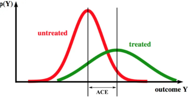
2.4 Illustration of the ACE. The ACE is the difference in average outcomes
over interventional distributionsFT =t(treated) and FT =c (untreated). 17
2.5 Causal graph of ignorable treatment assignment. . . 17
2.6 Causal graph of a sufficient covariateU. . . 18
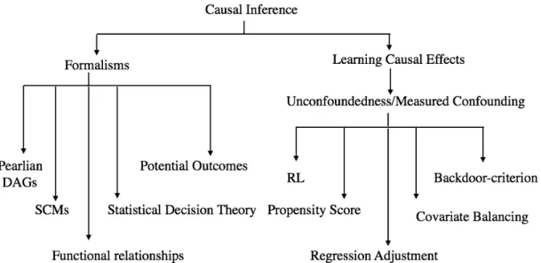
2.7 Summary of causal inference frameworks and methods for estimating
causal effects under measured confounding. . . 26
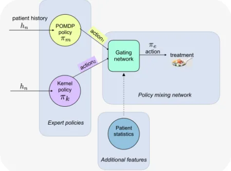
3.1 The mixture-of-experts framework for HIV therapy selection. We
com-bine policies at test time using a mixture-of-experts gating network that weights POMDP and kernel policies for each patient on the basis of their
history. . . 29
LIST OF FIGURES xi
3.2 (a) Distribution of drug combinations across training data. The
distribu-tion of treatments is considerably imbalanced. (b) Pruned distribudistribu-tion of most frequently occurring drug combinations from 1990 and 2000 across training data. Pruning the treatment space according to the periods in which drugs have been introduced and actively used produces a more
balanced distribution of therapies. . . 34
3.3 Interpreting the features of the mixture-of-experts network that have the
highest weights. The history length and quantile distances between pa-tients have the highest weight. The mixture-of-experts prefers the kernel policy for patients with short histories that are closer and more simi-lar to other patients as shown in (a). The mixture-of-experts prefers the POMDP policy when patients have longer histories that are distinct from
other patients as in (b). . . 37
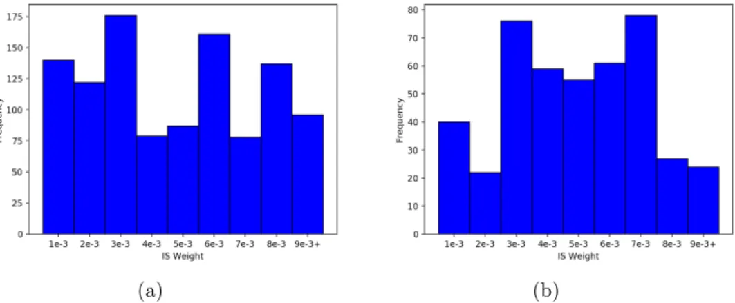
3.4 Distributions of frequencies of non-zero IS weights for (a) EIDB and (b)
SHCS data sets respectively. Overall, our treatments are fairly consistent with those in the data sets since the distributions are relatively balanced. 38
4.1 In our model-mixing approach, we create a simulator that chooses
be-tween parametric (discrete POMDP) and non-parametric (kernel) ap-proaches for performing the forward simulation and use this simulator for planning. Specifically we now incorporate knowledge from the kernel directly into estimation of belief states based on which we can infer suit-able treatments. The combined belief state representation here may be
viewed as a means of representing confounding for causal inference. . . . 45
4.2 Illustration of dynamics for the toy example. The optimal sequence of
actions for a type A variant is to initially take action 1 or 2, followed by action 1. For type B variants, the optimal sequence of actions is to first
take actions 1 or 2, followed by action 2. . . 49
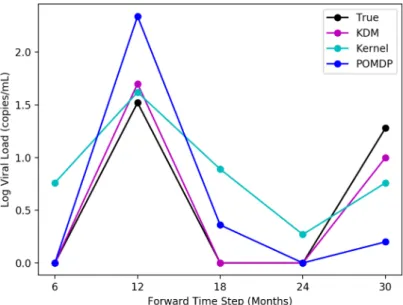
4.3 Simulating the viral load in an HIV patient when the viral load is below
detection limits (indicated by 0). KDM can detect the occurrence of blips at 12 and 30 months, unlike a MoE. No treatment change should
be administered here. . . 52
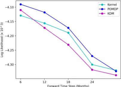
4.4 Comparison of predictive log-likelihood across baselines for HIV for a
typical test patient. KDM’s predictions are more accurate across the
forward time steps. . . 53
4.5 Box plot of viral load predictions across 3000 test patients under baselines
over a 30-month horizon. KDM’s predictions are closer to the ground
truth than POMDP or kernel predictions. . . 53
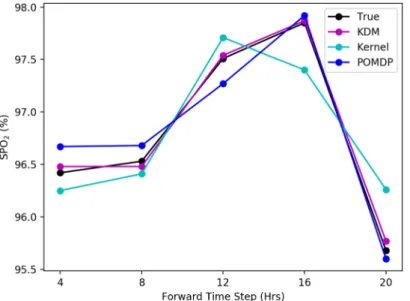
4.6 Simulating the SpO2of a sepsis test patient under baselines over a 20-hour
horizon. Counterfactual predictions of SpO2 levels are more accurate
using KDM than existing baselines. . . 56
4.7 Comparison of predictive log-likelihood across baselines for sepsis for a
typical test patient. KDM’s predictions are more accurate across the
forward time steps. . . 56
4.8 Box plot of SpO2 predictions across 3000 test patients under baselines
over a 20-hour horizon. KDM’s predictions are closer to the ground truth
4.9 Distributions of frequencies of non-zero IS weights for (a) HIV and (b) sepsis respectively. Our treatments are fairly consistent with those in the
data sets. . . 60
5.1 Influence diagram of the CEIB. Red and green circles correspond to
ob-served and latent random variables respectively, while blue rectangles
represent interventions. We identify a low-dimensional representation Z
of covariates X to estimate the effects of an intervention on outcome Y
where partial covariate information is available. . . 66
5.2 Graphical illustration of the CEIB. Orange rectangles represent deep
net-works parameterising the random variables . . . 67
5.3 (a) Information curves forI(Z;T) and (b)I(Z; (Y, T)) with de-randomised
and randomised data respectively. When the data is randomised, the
value ofI(Z;T) is close to zero. The differences between the curves
illus-trates confounding. When data is de-randomised, we are able to estimate
treatment effects more accurately by accounting for this confounding. . 72
5.4 Illustration of the proportion of major ethnic groups within the four
clus-ters. Grey and orange indicate de-randomised and randomised data re-spectively. For better visualisation, we only report the two main clusters which include the majority of all patients. The first cluster in (a) is a neutral cluster. The second cluster in (b) shows an enrichment of in-formation in the African-American group. Clusters 3 and 4 in (c) and (d) respectively, show an enrichment of information in the White group. Overall, the clusters exhibit a distinct structure with respect to the known ethnicity confounder. Moreover, each of the clusters is associated with different SCE values. In particular, the second cluster has a lower SCE which suggests that educational intervention for these members has less of an impact on outcomes – a result consistent with our de-randomisation
strategy. . . 73
5.5 Out-of-sample error in ACE with a varying number of clusters. . . 73
5.6 Subfigures (a) and (b) illustrate the information curveI(Z;T) andI(Z; (Y, T))
for the task of managing sepsis. We perform a sufficient reduction of the covariates to 6-dimensions and are able to approximate the ACE on the
basis of this. . . 74
5.7 Proportion of initial SOFA scores in each cluster. The variation in initial
SOFA scores across clusters suggests that it is a potential confounder of
LIST OF FIGURES xiii
5.8 Illustration of the proportion of HIV patients in each cluster according to
their number of past treatment lines [1, 2, 3, 4+] where 4+ corresponds to more having than 4 previous therapy combinations. The clusters differ in composition and in the SCE scores. In general clusters with a larger proportion of individuals who received more past therapies tend to have smaller SCEs. This suggests that PIs seem to have the largest impact on these patients. Patients frequently get treated with PI-boosted therapies as a result of previous treatment failures or other reasons for therapy switching such as side-effects. In contrast, patients with fewer past treat-ment lines are less likely to receive PI-boosted therapies because they are
unnecessary. . . 76
6.1 Diagram of gated recurrent unit (GRU) used for each timestep our neural
time-series model. The orange triangle indicates the predicted output ˆyt
at timet. . . 81
6.2 Overview of tree regularisation procedure. . . 83
6.3 2D Parabola task: (a) Each training data point in 2D space, overlaid with
true parabolic class boundary. (b): Each method’s prediction quality (AUC) and complexity (path length) metrics, across range of
regularisa-tion strength λ. In the small path length regime between 0 and 5, tree
regularisation produces models with higher AUC than L1 or L2. (c-e): Decision boundaries (black lines) have qualitatively different shapes for
different regularisation schemes, as regularisation strength λ increases.
We colour predictions as true positive (red), true negative (yellow), false
negative (green), and false positive (blue). . . 85
6.4 Toy Signal-and-Noise HMM Task: (a)-(c) Decision trees trained to mimic
predictions of GRU models with 25 hidden states at different
regulari-sation strengths λ; as expected, increasing λ decreases the size of the
learned trees (see supplement for more trees). Decision tree (c) suggests
the model learns to predict positive output (blue) if and only if “x[0] == 1
and x[3] == 1 and x[4] == 0”, which is consistent with the true rule we
used to generate labels: assign positive label only if first dimension is on
(x[0] == 1) and first state is active (emission probabilities for this state:
[.5 .5 .5 .5 0 . . .]). (d) Tree-regularised GRU models reach a sweet spot
of small path lengths yet high AUC predictions that alternatives cannot
reach at any tested value ofλ. . . 87
6.5 Sepsis task: Study of different regularisations for GRU model with 100
states, trained to jointly predict 5 binary outcomes for ICU patients. Panels (a) and (c) show AUC vs. path length for 2 of the 5 outcomes (remainder in the supplement); in both cases, tree-regularisation provides higher AUC in the target regime of low-complexity decision trees. Panels
(b) and (d) show proxy trees for the tree-regularised GRU (λ= 2 000);
6.6 TIMIT and HIV tasks: Study of different regularisation techniques for GRU model with 75 states. Panels (a)-(c) are tradeoff curves showing how AUC predictive power and decision-tree complexity evolve with in-creasing regularisation strength under L1, L2 or tree regularisation on both TIMIT and HIV tasks. The GRU is trained to jointly predict 15 binary outcomes for HIV, of which 2 are shown here in Panels (b) - (c).
The GRU’s decision tree proxy for HIV Adherence is shown in (d). . . . 89
6.7 Prediction quality (AUC) vs. complexity (path length) for the
GRU-HMM over a range of regularisation strengths λ. Subtitles show the
number of HMM states and GRU states. See earlier figures to compare
these GRU-HMM numbers to simpler GRU and decision tree baselines. 90
7.1 Summary of causal inference frameworks and methods for estimating
causal effects under measured and hidden confounding. The work in our thesis only addressed measured confounding. Possible extensions to scenarios with hidden confounding include the use of directed information
in our RL models and instrumental variables. . . 95
B.1 True average path lengths (yellow) and surrogate estimates ˆΩ (green)
across many iterations of network parameter training iterations. . . 102
B.2 This figure shows the effects of weight augmentation and retraining. The blue line is the true average path length of the decision tree at each epoch. All other lines show predicted path lengths using the surrogate MLP. By randomly sampling weights and intermittently retraining the surrogate, we significantly improve the ability of the surrogate model to track the
changes in the ground truth. . . 103
B.3 Emission (5 states vs 7 features) and transition probabilities for the signal HMM (a, b) and noise HMM (c, d). . . 104 B.4 Performance and complexity trade-offs using L1, L2, and Tree
regularisa-tion on (a) GRU and (b) GRU-HMM performance on the Signal-and-noise HMM dataset. Note the differences in scale. . . 105 B.5 Decision trees trained under varying tree regularisation strengths for
GRU models on the signal-and-noise HMM dataset dataset. As the tree regularisation increases, the number of nodes collapses to a single one. If we focus on (h), we see that the tree resembles the ground truth data-generating function quite closely. . . 106 B.6 Performance and complexity trade-offs using L1, L2, and Tree
regular-ization on GRU performance on the Sepsis dataset. . . 106
B.7 Decision trees trained using λ = 800.0 for a GRU model using Sepsis.
The 5 output dimensions are jointly trained. . . 107 B.8 Performance and complexity trade-offs using L1, L2, and Tree
regular-isation on GRU for the HIV dataset. The 5 outputs shown here were trained jointly. . . 109 B.9 (a) Performance and complexity trade-offs using L1, L2, and Tree
reg-ularisation for GRU models on TIMIT. (b) Decision tree trained using
λ= 500.0 tree regularization on GRU. . . 111
B.10 Deep residual model: GRU-HMM. The orange triangle indicates the out-put used in surrogate training for tree regularization. . . 111
LIST OF FIGURES xv B.11 Performance and complexity trade-offs using L1, L2, and Tree
regular-ization on GRU-HMM performance on the Sepsis dataset. . . 113
B.12 Decision trees trained using Tree regularization (λ= 2000.0) from
GRU-HMM predictions on the Sepsis dataset. . . 113
B.13 HIV task: Study of different regularisation techniques for GRU-HMM
model with 75 GRU nodes and 25 HMM states, trained to predict whether
CD4+ ≤ 200 cells/ml. (a) Example decision tree for λ = 1000.0. (b)
Example decision tree forλ= 3000.0. The tree in (b) is slightly smaller
than the tree in (a) as a result of the regularisation. . . 113
B.14 TIMIT task: Study of different regularisation techniques for GRU-HMM
model with 75 GRU nodes and 25 HMM states, trained to predict STOP phonemes. (a) Tradeoff curves showing how AUC predictive power and decision-tree complexity evolve with increasing regularisation strength
under L1, L2, or Tree regularisation. (b) Example decision tree for λ=
3000.0. (c) Example decision tree forλ= 7000.0. When comparing with
figure B.9b, this tree is significantly smaller, suggesting that the GRU performs a different role in the residual model. . . 114 B.15 Decision trees from 10 independent runs on the signal-and-noise HMM
dataset with λ= 0.01. With low regularisation, the variance in tree size
and shape is high. . . 115 B.16 Decision trees from 10 independent runs on the signal-and-noise HMM
dataset withλ= 1000.0. Seven of the ten runs resulted in a tree of the
same structure. The other three trees are similar, often having additional subtrees but sharing the same splits and features. . . 115
1.1 The 3-level hierarchy of tools for modelling causality (Pearl, 2018). P(y|x)
is the probability of outcome Y = y given an observation X = x.
P(y|do(x), z) refers to the probability of Y = y given that we
explic-itly intervene and set X to x and subsequently observe Z = z. Here,
Px(y|x0, y0) refers to the probability of Y =y had X been x given that
we observeX asx0 and Y asy0. . . . 2
2.1 Illustration of Simpson’s paradox. Treatment B appears better overall
despite performing worse on patients with both large and small kidney
stones (Charig et al., 1986). . . 11
3.1 Off-policy evaluation using importance sampling, weighted importance
sampling and doubly robust methods for different therapy selection
mod-els across EIDB test set (γ = 0.98). Overall, the mixture-of-experts
produces the largest immune response while reducing the viral load. . . 36
3.2 Off-policy evaluation using importance sampling, weighted importance
sampling and doubly robust methods for different therapy selection
mod-els across SHCS test set (γ = 0.98). The mixture-of-experts produces
the largest immune response while reducing the viral load on a different
cohort of patients. . . 36
3.3 Feature weights for mixture-of-experts gating function. The history length
and quantile distance have the largest weights. . . 37
3.4 Percentages of mixture-of-expert policies in violation with clinical
recom-mendations. . . 39
4.1 Performance comparison of KDM vs. baselines across 250 test sequences
for the toy example. A higher value corresponds to a higher accumulated
reward, and indicates a better performing policy. . . 50
4.2 Summary of HIV cohort statistics. . . 50
4.3 Performance comparison of KDM vs. baselines for HIV therapy selection
across 3000 held-out patients using a POMDP model with 30 states. KDM produces the largest immune response while reducing the viral
load, thus outperforming its competitors. . . 51
4.4 Summary of sepsis cohort statistics . . . 54
LIST OF TABLES xvii
4.5 Performance comparison of KDM vs. baselines for treating sepsis across
3000 held-out patients using a POMDP model with 75 states. The KDM policy significantly reduces the odds of mortality (indicated by a lower
value here), and outperforms existing baselines. . . 55
4.6 Friedman’s test measuring predictive performance differences of KDM
against POMDP and kernel methods acrosstin HIV. Bold p-values
cor-respond to steps where counterfactual predictions from KDM are signif-icantly more accurate than the respective methods. Comparisons with policy-based approaches like the mixture-of-experts cannot be drawn here
as these methods cannot be used for counterfactual predictions. . . 58
4.7 Friedman’s test measuring predictive performance differences of KDM
against POMDP and kernel methods across t in sepsis. Bold p-values
correspond to steps where counterfactual predictions from KDM are sig-nificantly more accurate than the respective methods. Comparisons with policy-based approaches like the mixture-of-experts cannot be drawn here
as these methods cannot be used for counterfactual predictions. . . 58
5.1 (a) Within-sample and out-of-sample mean and standard errors in ACE
across models on the complete IHDP data set. A smaller value indi-cates better performance. Bold values indicate the method with the best performance. (b) Within-sample and out-of-sample mean and standard errors in ACE across models using a reduced set of 22 covariates at test
time. . . 71
6.1 Fidelity of predictions from our trained deep GRU-RNN and its
cor-responding decision tree. Fidelity is defined as the percentage of test examples on which the prediction made by a tree agrees with the deep model (Craven & Shavlik, 1996). We used 20 hidden GRU states for
signal-and-noise task, 50 states for all others. . . 92
A.1 Performance comparison of mixture-of-experts vs. baselines for HIV ther-apy selection across 3 000 held-out patients using a POMDP model with
30 states using reward criterion (a) (γ = 0.98). The mixture-of-experts
still produces the largest immune response while reducing the viral load,
regardless of whether a larger weight is given to CD4+ orV
t (γ = 0.98). 99
A.2 Performance comparison of mixture-of-experts vs. baselines for HIV ther-apy selection across 3 000 held-out patients using a POMDP model with
30 states using reward criterion (b) (γ = 0.98). Performance of the
mixture-of-experts has significantly higher variance when placing a higher weight on the number of mutations. Evidently in this case, the
mixture-of-experts does not always lead to the best immune response. . . 99
A.3 Off-policy evaluation using importance sampling, weighted importance sampling and doubly robust methods for different therapy selection mod-els across EuResist test set using an unpruned treatment distribution of
A.4 Off-policy evaluation using importance sampling, weighted importance sampling and doubly robust methods for different therapy selection mod-els across SHCS test set using an unpruned treatment distribution of
treatments (γ = 0.98). . . 100
B.1 Dataset summaries and training parameters used in our experiments. . . 103 B.2 Performance metrics across models on the signal-and-noise HMM dataset.
The parameter count is included as a measure of the model capacity. . . 107 B.3 Performance metrics for multi-dimensional classification on a held-out
portion of the Sepsis dataset. Total Average Path Length refers to the
summed average path lengths across the 5 output dimensions. Refer to Fig. B.6 for average-path-lengths split across dimensions. . . 108 B.4 Performance metrics for multi-dimensional classification on a held-out
portion of the HIV dataset. Total Average Path Length refers to the
summed average path lengths across the output dimensions. . . 110 B.5 Performance metrics across models on a held-out portion of the TIMIT
dataset. . . 112 B.6 Training time for recurrent models measured against all datasets used
in this paper. Epoch time denotes the number of seconds it took for a single pass through all the training data. The epoch times for GRU-TREE and GRU-HMM-GRU-TREE include surrogate training expenses. If we retrain sparsely, then the cost of surrogate training is amortized and the epoch time for GRU and GRU-TREE, GRU-HMM and GRU-HMM-TREE are approximately the same. To measure epoch time, we used 10 HMM states, 10 GRU states, and 5 of each for GRU-HMM models. We trained the surrogate model for 5000 epochs. These tests were run on a single Intel Core i5 CPU. . . 114
Chapter 1
Introduction
1.1
General Motivation
Machine learning has enabled us to answer many questions and vastly revolutionised several disciplines such as computer vision. The majority of these tasks have been tack-led using training sets of data and prediction functions to identify a set of associations in the data. While associations may be useful for making accurate predictions, in fields such as medicine however, the driving questions are most often not associational, but
rathercausal in nature (Pearl et al., 2009). For instance, what is the effect of a drug on
a particular individual or population? What would happen if a patient exhibited differ-ent symptoms to those observed? Does a particular genetic mutation cause resistance against a certain drug? Each of these questions is rooted in acquiring a deeper under-standing of the reasons for a particular event, and may thus be referred to as causal inference or discovery questions. For such questions, understanding the distinction be-tween association and causation is crucial. To illustrate the difference here, consider the following example from Guo et al. (2018). When temperatures are high, an ice-cream shop owner may observe both high sales and high electricity bills. While there may be a strong association between the electricity bill and sales, it is unlikely that the elec-tricity bill is the cause of high sales. This could be demonstrated by observing what happens if the lights are left on for a prolonged period of time. Evidently, there would be no impact on sales. Rather, the association between sales and the electricity bill
may be explained by a common cause variable orconfounder, namely the temperature:
If temperatures are high, there is a higher demand for ice-cream and more electricity is required to cool the increased supply. In this example, conducting an experiment to distinguish between cause and association is straightforward. In practice however, performing such experiments to reason about potential causes is not always possible. Causal discovery questions are generally challenging and cannot be answered solely on the basis of data, since they require some knowledge of the underlying data generating mechanism (Pearl et al., 2009).
To distinguish between tools for associational modelling and causal modelling, Pearl (2018) introduces a 3-level hierarchy based on the kind of information required to an-swer questions at each level. The three levels are: i) Association, ii) Intervention and iii) Counterfactuals. Table 1.1 illustrates this hierarchy, as well as examples of
ques-tions at each level. For instance, the first level identifies statistical relaques-tions solely on
the basis of data, and can thus be used to determine associations. These are quantities
such as correlations, odds ratios, risk ratios and statistical dependencies (Pearl et al., 2009). Since questions at the first level are entirely associational, they can typically be addressed with existing machine learning techniques such as regression. The next
level, Intervention, focuses on understanding the effects of causes. Specifically, it
re-quires not only observing existing data, but actively doing something to reason about the effects of interventions. The final layer, namely counterfactuals, may be used to
reason about thecauses of effects. Questions at this level involve retrospection and
typ-ically cannot be answered using associational or interventional information alone; for example, given a control experiment where patients are assigned particular treatments, we usually cannot re-execute the experiment to see what would have happened had the patient been treated otherwise. Rather, these questions require explicitly modelling the underlying data generation procedure and using such a model to make inferences. Overall, the hierarchy may viewed as directional since questions from a particular level can be addressed if information from that level or subsequent levels is available. That is, a model for counterfactuals can be used to address questions concerning the effects of interventions and identify associations, but the opposite does not necessarily hold. A schematic representation of this relationship is shown in Figure 1.1. Here, accounting for interventions by reasoning about their effects and learning causal models subsumes the task of identifying associations and making predictions.
Level Typical Activity Typical Questions Examples
1. Association Seeing What is? What does a symptom tell us
P(y|x) e.g. Regression How doesX about the disease?
change my belief inY?
2. Intervention Doing, What if? What if I take aspirin, will
P(y|do(x), z) Intervening What if I doX? my headache be cured?
e.g. Reinforcement Learning
3. Counterfactuals Imagining, Was itXthat causedY? Was it aspirin that
Px(y|x0, y0) Retrospection What if I acted differently? stopped my headache?
e.g. Structural Causal Models
Table 1.1: The 3-level hierarchy of tools for modelling causality (Pearl, 2018). P(y|x)
is the probability of outcome Y =y given an observation X =x. P(y|do(x), z) refers
to the probability of Y = y given that we explicitly intervene and set X to x and
subsequently observeZ =z. Here,Px(y|x0, y0) refers to the probability ofY =y hadX
beenx given that we observe X asx0 and Y asy0.
One of many principled ways to formulate queries concerning causation is using
Structural Causal Models (SCMs)(Pearl, 1995, 2009). In its general form, an SCM
denoted (U,V, F) consists of two sets of variables U and V, and a set of functions fi
that define or simulate how values are assigned to Vi ∈ V. For example, vi = fi(u, v)
describes the process of how vi is assigned a value based on the values u, v and the
function fi. The variables U are known as exogenous noise variables whose values
are determined by external influences beyond the model, while the variables V are
endogenous variables whose values are defined by other variables in the model. SCMs are frequently illustrated as causal graphs that capture the causal relationships over the variables. In the past, SCMs have found applications across domains such as economics (e.g. Imbens (2004)), social sciences (e.g Duncan (1975); Goldberger (1972); L. Morgan & Winship (2007)) and education (e.g. Dehejia & Wahba (1999); Hill (2011a); LaLonde
1.2. CAUSAL INFERENCE FOR PERSONALISED MEDICINE 3 (1986)).
Figure 1.1: Illustration of the relationship between causal and associational modelling (adapted from Peters et al. (2017)). Causal models can be used to make predictions about the effects of interventions or (in some cases) counterfactual claims about a sys-tem. This requires modelling dependence relations as well as performing interventions, and hence subsumes probabilistic reasoning. Standard probabilistic models can account for associations but not for interventions. The orange boxes indicate how these models relate to Pearl’s hierarchy.
1.2
Causal Inference for Personalised Medicine
In this thesis, we focus on the role of causal knowledge in healthcare, particularly for personalising treatments to a patient’s needs. The fundamental question we address is:
What is the effect of a therapy on a particular patient? We study this question in the
context of two healthcare applications, namely treating patients with sepsis and Human Immunodeficiency Virus (HIV). We specifically introduce different causal models for this purpose. These models may be viewed as tools from either the Intervention or Counterfactual level in Pearl’s hierarchy. In the following sections, we briefly introduce both healthcare applications and identify the major challenges in these domains. We subsequently embed these in the context of causal inference and machine learning, and highlight the key contributions of this thesis.
1.2.1 Human Immunodeficiency Virus
HIV1 is a retrovirus that currently affects more than 36 million people worldwide and
causes Acquired Immune Deficiency Syndrome (AIDS) (UNAIDS, 2015). If untreated, HIV attacks and destroys the immune system by causing progressive loss of white blood
cells, such as CD4+ T-lymphocytes. The gradual destruction of the immune system
leaves a patient vulnerable to opportunistic infections that frequently result in death.
Figure 1.2: The viral genome of HIV. The Pol region serves as an active site for PIs, RTIs and Integrase Inhibitors (Freed, 2004).
To date, the only practical treatment for HIV is through life-long administration of com-binations of antiretrovirals, known as Highly Active Antiretroviral Therapy (HAART), that target various phases of the viral life cycle. There are currently more than 20 drugs
in use for HAART (G¨unthard et al., 2016). These may be classified as: Entry/Fusion
Inhibitors, Reverse Transcriptase Inhibitors (RTIs), Integrase Inhibitors and Protease Inhibitors (PIs). Entry Inhibitors try to stop viral entry into an immune cell (De Clercq, 2009). RTIs bind to the virus’s reverse transcriptase enzyme, thereby preventing the virus from converting its genomic material into DNA. Integrase Inhibitors prevent the viral DNA from integrating with the host’s genome by inhibiting the function of the integrase enzyme in the virus (Lusic & Siliciano, 2017). Protease inhibitors target the formation and assembly of viral proteins that are crucial for assembling new viral par-ticles (Hammer et al., 2006). Figure 1.2 illustrates the target sites of these drugs on the HIV genome. Overall, advances in drug therapies since the introduction of HAART in 1996, have meant that many individuals are able to suppress viral loads below detection
limits (<40 copies/ml) and sustain immune functionality for prolonged periods of time.
1.2.2 Challenges with Treating HIV
High Mutagenicity. Despite the introduction of new antiretrovirals, the high
evolu-tionary dynamics of the virus enable it to escape drug pressure by acquiring resistance mutations (Mansky & Temin, 1995). Resistance to a particular drug may also result
in resistance to other drugs from the same family; this is known as cross-resistance
(Thompson et al., 2010). This, together with the large number of available therapy combinations makes manually searching for an effective therapy particularly challeng-ing.
Patient Heterogeneity. HIV may be classified into four groups, M, N, O and P
(Robertson et al., 2000). Of these, group M accounts for the majority of the global pandemic and consists of ten different subtypes, A-K. However, many new recombinant strains can be formed from further recombination between subtypes in a host. Overall,
1.2. CAUSAL INFERENCE FOR PERSONALISED MEDICINE 5 HIV’s high rate of mutation means that a patient may harbour many genetically hetero-geneous populations that continue evolving. As a result, causal inference is important to tailor treatments to a patient’s individual responses.
Influence of Confounding Factors. Existing sources of HIV data are high-dimensional
and frequently biased by several confounding factors such as different treatment back-grounds, varying levels of therapy experience, demographics, and the occurrence of co-infections e.g. tuberculosis. These factors necessitate causal inference to reason about patient outcomes and administer appropriate therapies.
1.2.3 Sepsis
Sepsis is a complex multi-system disease resulting from the body’s inflammatory re-sponse to infection (Brand et al., 2017). Treating patients suffering from sepsis is par-ticularly challenging since they tend to exhibit a myriad of symptoms, depending on the nature of infection. In spite of this heterogeneity, sepsis is typically characterised by conditions such as a rapid rise or fall in body temperature, an elevated heart rate (known as tachycardia), vasodilation, hypotension and an elevated white blood cell count (Polat et al., 2017; Singer et al., 2016). The most severe form of sepsis, known as septic shock, occurs when patients experience severe hypotension that potentially results in organ dysfunction or failure. Septic shock is one of the leading contributors to mortality in the ICU with global estimates of between 20 and 30 million cases annually, and mortality rates typically exceeding 50% (Napolitano, 2018; Polat et al., 2017). As a result, sepsis is frequently viewed as a medical emergency that requires immediate intervention.
Treatments for sepsis vary depending on the underlying nature of infection, and in practice there is often little consensus about how patients should be treated (Peng et al., 2019). However, antibiotics, intravenous fluid resuscitators, corticosteroids and mechanical ventilation are typically necessary for combating hypotension and tachycar-dia (Hajj et al., 2018). When fluid resuscitation alone fails, vasopressors are frequently administered to restore adequate blood pressure and correct for excessive vasodilation (Brand et al., 2017). Depending on the severity of infection and loss of blood pressure, a number of vasopressors may be administered concurrently. These include dopamine, epinephrine, phenylephrine and vasopressin however, norepinephrine is frequently used as a first-line therapy (Brand et al., 2017). Overall, administering vasopressors for treat-ing sepsis is particularly challengtreat-ing, since vasopressors are associated with a number of dangerous outcomes such as fluid overload, kidney failure, high blood pressure and irregular heartbeat, all of which can have severe implications on a patient’s mortality.
1.2.4 Challenges with Treating Sepsis
Patient Heterogeneity. The primary challenge of treating patients with sepsis is
the lack of consensus as to what symptoms characterise the disease. Overall, sepsis can occur as a result of bacteria, viruses or parasites, severe trauma, pneumonia or other infections, and patients with each of these conditions may exhibit a wide variety of clinical and physiopathological symptoms (Polat et al., 2017). For these reasons, there is no universal diagnosis of the disease. As a result, the definition of sepsis has progressively evolved over the past thirty years to include new signs and symptoms (Napolitano, 2018).
Currently, an ICU patient may be classified as septic if they experience the following conditions: i) an increase in their sequential organ failure assessment score (known as SOFA) of more than 2 points; ii) a systolic blood pressure of less than 100 mmHg; iii) a respiratory rate of more than 22; iv) an altered mental state of less than 15 defined by the Glasgow Coma Scale (GCS) (Singer et al., 2016). Still, these criteria are difficult to use in practice and may not necessarily promote an understanding of the underlying disease process. In such scenarios, causal reasoning is important to understand how patients should be treated.
Influence of Confounding Factors. While sepsis is associated with a high mortality
rate, it is also common for sepsis survivors to be re-admitted to hospital shortly after they are discharged. Not only do these patients have a higher chance of infection, but also have higher levels of inflammation – factors that may ultimately compromise quality of life and affect long-term life expectancy (Shankar-Hari et al., 2016). That is, a patient’s outcomes following sepsis typically reflect a complex interplay between several factors such as their demographics, treatments in ICU, post-ICU care and the nature of initial infection. In such cases, identifying these factors and correcting for their influences may provide a better understanding of the disease and inform more effective interventions. Like with HIV, observational data of patients suffering from sepsis may be useful to promote such an understanding of the disease however, these too are biased by confounding. As a result, causal inference is crucial to be able to reason about patient outcomes and infer appropriate treatment strategies.
1.3
Contributions and Outline of the Thesis
Our overall aim is to understand the effect of a therapeutic intervention on a patient with HIV or sepsis. Consequently, our work is rooted in three closely related themes
namely,causal inference,explainability anddecision-making. In this thesis, we examine
the relationship between these themes. In particular, we view both explainability and decision-making in light of causal inference as shown in Figure 1.3. While the use of machine learning in everyday systems is becoming increasingly common, the ability of
a system to explain its reasoning is crucial in high-stake domains such as healthcare.
That is, if we can interpret or explain why a system makes its predictions, we can verify whether or not this reasoning is correct (Doshi-Velez & Kim, 2017). Unfortunately however, there is little agreement on what model explainability is and how it should be evaluated. Similarly, in domains where decision-making is challenging, we usually require a deeper understanding of the effects of executing a particular decision before determining a suitable course of action. Causal reasoning may be helpful for tackling both of these issues simultaneously.
This thesis is divided into roughly three parts. In the first part of the thesis, we examine the problem of HIV therapy selection. Here, we show how tools from the Intervention layer of Pearl’s hierarchy such as reinforcement learning (RL), can be com-bined with existing methods for associational modelling to reason about the effects of therapies. While in the past, the problem of HIV therapy selection has been stud-ied extensively using regression methods, coupling this associational knowledge with RL enables us to personalise HIV therapies on the basis of a patient’s history, while simultaneously accounting for the effects of confounders. In the second part of this
1.3. CONTRIBUTIONS AND OUTLINE OF THE THESIS 7
Figure 1.3: Illustration of the relationship between causal inference, decision-making and explainability. Explanations can aid decision-making if they are easy to under-stand and simple enough to be parsed. Similarly, reinforcement learning may be used to provide explainable recommendations via policies that are easy to step through, thus aiding decision-making. Causal inference is important for both explainability and decision-making since knowledge about interventions and their effects enables us to obtain meaningful explanations and informs better decisions.
thesis, we additionally study the problem of treating patients with sepsis. Here, we
consider an alternative view to counterfactuals known as decision-theoretic causality
which, like tools from the Intervention layer, enables us to directly examine the effects of an intervention. Specifically, we learn a low-dimensional compact representation of confounding that allows us to accurately estimate the effects of a therapy where only partial information is available. Finally, in the last part of this thesis, we introduce a new tree-based regularisation strategy for medical decision-making such that humans may step through and understand the predictions a system makes. Using both HIV and sepsis as application domains, we show that such explainability is important as it may shed light on the effects of interventions and allow us to tailor therapies to a patient’s responses accordingly.
Having presented a brief overview of the thesis, we provide a detailed roadmap of how this thesis is structured. Chapter 2 serves as a general introduction to causal inference and provides an overview of two different perspectives of the field, namely
thepotential outcomes framework anddecision-theoretic causality. We specifically show
how both these views are related to Pearl’s 3-level hierarchy and the theory of SCMs, as well as how they relate to each other. In the second part of Chapter 2, we introduce the RL framework which serves as the basis for two of our contributions in this thesis. In particular, we show that RL may also be expressed in terms of an SCM under certain conditions, thereby establishing a link between the Interventional and Counterfactual layers of the hierarchy. We subsequently describe how to perform inference and evaluate policies with such a model.
associational modelling in a mixture-of-experts model to learn treatment policies for patients with HIV. In particular, the mixture-of-experts selectively alternates between a non-parametric expert and a parametric RL expert to personalise therapies according to a patient’s particular needs. This approach is extended in Chapter 4 where we present our second major contribution. Here, instead of combining therapy policies as we do in Chapter 3, we directly incorporate the knowledge from associational modelling into an RL model to learn a more powerful causal model that we can use to generate counterfactuals and perform ‘what-if’ reasoning. This model allows us to simultaneously address patient heterogeneity and account for the effects of confounding. We then show how such a model can be used to infer state-of-the-art treatment strategies for both HIV and sepsis.
While the work in Chapter 3 and 4 combines different representations of causal knowledge with machine learning to learn better treatment policies, in Chapter 5 we shift our focus to learn better representations of confounders themselves. Specifically, we introduce our third major contribution, a variant of the Information Bottleneck method (Tishby et al., 2000) to learn a low-dimensional latent compression of confounding, and show how such a compression enables us to estimate both the average and specific causal effects of an intervention, even where covariate information is incomplete at test time. We subsequently apply this method to several benchmark problems as well as the tasks of treating sepsis and HIV.
Chapter 6 describes our final contribution where we introduce tree-based regularisa-tion to optimise models for human simulatability. Importantly, this technique enforces that the predictions made by a model are explainable in terms of small decision-trees which can be traced through and audited. We demonstrate the importance of such ex-plainability for decision-making and understanding treatment effects on both HIV and sepsis tasks. The thesis is concluded in Chapter 7 with a summary and a discussion on limitations of our work, as well as future research directions.
1.4
List of Publications
The following papers have resulted from some of the work presented in this thesis.
• Cause-Effect Deep Information Bottleneck For Systematically Missing Covariates
Sonali Parbhoo, Mario Wieser, Aleksander Wieczorek, Volker Roth Under review, 2019.
• Regional Tree Regularization for Interpretability in Black Box Models
Mike Wu, Sonali Parbhoo, Michael C. Hughes, Ryan Kindle, Leo Celi, Maurizio Zazzi, Volker Roth, Finale Doshi-Velez
Under review, 2019.
• Intelligent Policy Mixing for Improved HIV-1 Therapy Selection
Sonali Parbhoo, Jasmina Bogojeska, Mario Wieser, Fabricio Arend Torres, Maur-izio Zazzi, Susana Posada Cespedes, Niko Beerenwinkel, Enos Bernasconi, Manuel Battegay, Alexander Calmy, Matthias Cavassini, Pietro Vernazza, Andri Rauch,
Karin J. Metzner, Roger Kouyos, Huldrych G¨unthard, Finale Doshi-Velez, Volker
Roth
1.4. LIST OF PUBLICATIONS 9
• Generative Subspace Learning Under Irrelevance Constraints in Continuous
Do-mains
Mario Wieser, Sonali Parbhoo, Aleksander Wieczorek, Volker Roth Under review, 2019.
• Determinants of HIV-1 Reservoir Size and Long-Term Dynamics
Nadine Bachmann, Chantal von Siebenthal, Valentina Vongrad, Teja Turk, Kathrin Neumann, Niko Beerenwinkel, Jasmina Bogojeska, Jacques Fellay, Volker Roth, Yik Lim Kok, Christian Thorball, Alessandro Borghesi, Sonali Parbhoo, Mario Wieser, Jurg Boni, Matthieu Perreau, Thomas Klimkait, Sabine Yerly, Manuel Battegay, Andri Rauch, Matthias Hoffmann, Enos Bernasconi, Matthias Cavassini,
Roger Kouyos, Karin Metzner, Huldrych G¨unthard.
To appear in Nature Communications, 2019.
• Greedy Structure Learning of Hierarchical Compositional Models
Adam Kortylewski, Aleksander Wieczorek, Mario Wieser, Clemens Blumer, An-dreas Morel-Forster, Sonali Parbhoo, Volker Roth and Thomas Vetter.
To appear at CVPR, 2019.
• Improving Counterfactual Reasoning with Kernelised Dynamic Mixing Models
Sonali Parbhoo, Omer Gottesman, Andrew Slavin Ross, Matthieu Komorowski, Aldo Faisal, Isabella Bon, Volker Roth, Finale Doshi-Velez
PLoS One, Volume 13, Number 11, 2018.
• Beyond Sparsity: Tree Regularization of Deep Models for Interpretability
Mike Wu, Michael C. Hughes, Sonali Parbhoo, Maurizio Zazzi, Volker Roth, Finale Doshi-Velez
In Proceedings of the 32nd AAAI Conference on Artificial Intelligence, 2018.
• Combining Kernel and Model Based Learning for HIV Therapy Selection
Sonali Parbhoo, Jasmina Bogojeska, Maurizio Zazzi, Volker Roth, Finale Doshi-Velez
AMIA Summits on Translational Science Proceedings, 2017.
• Bayesian Markov Blanket Estimation
Dinu Kaufmann, Sonali Parbhoo, Aleksander Wieczorek, Sebastian Keller, David Adametz, Volker Roth
In Proceedings of the 19th International Conference on Artificial Intelligence and Statistics, 2016.
Related Work
2.1
Introduction
In the first chapter, we discussed the notion of causality and its relevance for estimating treatment effects in the context of both HIV and sepsis. In particular, we emphasised the
difference between seeing and doing using Pearl’s hierarchy: Seeing involves passively
observing a system in its natural condition; conversely, doing concerns the resulting
behaviour of a system when it is disturbed uponactive intervention. However, despite
the widespread usage of statistics to address queries about association and seeing, there is little consensus as to how queries of causation and doing should be formalised. As a result, over the years several different formalisms for causal inference have been pro-posed. One such formalism is SCMs that we introduced in Chapter 1. In this chapter we focus on two different formalisms of causality, namely statistical decision theory and the potential outcomes framework. We specifically discuss the main theoretical concepts required for understanding the subsequent work presented in this thesis. We also draw links between causal inference and other machine learning methods for decision-making such as reinforcement learning, as well as supervised learning that appear in Chapters 3, 4 and 6.
2.2
Confounding and Simpson’s Paradox
In healthcare, Randomised Control Trials (RCTs) are frequently viewed as the ‘gold standard’ for addressing causal questions and performing inference. The basic idea is to divide a set of patients into treatment and control groups. Patients from the treatment group are treated with a drug of interest, while patients from the control group are not allocated an intervention (termed a placebo control). The effects of the drug may then be assessed by comparing the outcomes of patients receiving treatment with the outcomes of those that do not. However, controlled experiments suffer from several drawbacks: they are expensive to conduct, may be ethically infeasible, are frequently susceptible to patient dropouts, and must typically be performed over several years. Alternatively, we must rely on observational data to draw inferences. However, in observational studies, the conditions across treatment groups may differ from those conditions we are interested in, and the characteristics of the individual subjects may not directly be comparable (Dawid, 2007a). As a result, it may be difficult to assess whether a particular effect is a direct result of an intervention or a consequence of other uncontrolled causes.
2.3. FORMAL FRAMEWORKS FOR CAUSALITY 11 Consider the example of treating kidney stones (Charig et al., 1986). Table 2.1 shows the success of surgery (treatment A) vs. percutaneous nephrolithotomy (treatment B). While at first, treatment B seems appears more successful, it tends to be prescribed to patients with smaller, less severe, kidney stones. Is treatment B more effective, or is its success rate a consequence of being applied selectively to milder conditions? If we further divide the data on the basis of stone size, treatment A now achieves a better success rate for both patients with large and small kidney stones. This is known as Simpson’s paradox (Simpson, 1951).
Treatment Overall Patients with small stones Patients with large stones
A 78% (273/350) 93%(81/87) 73%(192/ 263)
B 83%(289/350) 87% (234/270) 69% (55/80)
Table 2.1: Illustration of Simpson’s paradox. Treatment B appears better overall despite performing worse on patients with both large and small kidney stones (Charig et al., 1986).
Causal inference entails drawing conclusions based on responses to such interventions
(Dawid, 2010). At its core, causal reasoning is centred around the concept of
confound-ing. The example in Table 2.1 demonstrates the occurrence of confounding, where an
observed outcome in the data may be a true effect, but may also be a result of several other factors that vary with the actual cause. These factors may sometimes be referred
to asconfounding variables whose consequences distort the true effect of an intervention.
Together, the overall infeasibility of performing RCTs and the prevalence of confounding in observational data requires formalising the principles of causal inference.
2.3
Formal Frameworks For Causality
Several formal frameworks for causality have been proposed over the last few decades in an attempt to improve the rigour in addressing causal questions. These include graphical representations or causal diagrams, functional causal models, counterfactual models or models based on potential outcomes, and models based on statistical decision theory. We briefly describe each of these here before presenting more details in subsequent sections.
Graphical representations and causal diagrams are directed graphs that are used to visualise the causal relationships between variables in a model. Various different
graphi-cal representations have been proposed in e.g. Dawid (2002); Hern´an & Robins (2006b);
Pearl (2009). Functional causal models represent outcomes or effects of an intervention as a function of direct causes and some noise (Dawid, 2007a). In general, functional models assume that causal relationships can be represented entirely using deterministic functional equations; probabilities are introduced specifically under the assumption that certain variables are unobserved (Pearl, 2009). That is, the outcome is entirely deter-ministic given complete knowledge of the direct causes. SCMs are based on the idea of functional relationships, but coupled with graphical representations. Statistical mod-els, unlike functional modmod-els, assume that there is always a degree of uncertainty that must be modelled, irrespective of whether a variable is observed or not. In particular, the decision-theoretic view of causal inference is based on probabilities and statistical modelling where the effect of a treatment is seen as the difference between two different
probability distributions (Dawid, 2007a). Finally, counterfactual models measure causal effects as the difference between outcomes for an individual had they both taken and not taken the treatment (Sekhon, 2008). By definition, both of these outcomes cannot be observed simultaneously on a unit level, which necessitates joint probabilistic modelling
of the underlying data distribution in order to make inferences1.
Each of these frameworks has its merits, however we focus particularly on the decision-theoretic view of causal inference, and the counterfactual or potential out-comes perspective here. These formalisms differ in that they address different kinds of questions: the former can be used to address questions about effects of causes and is the primary focus of this thesis. In particular, when posing an effects-of-causes query,
we ask a hypothetical question such as: What would happen to my condition if I take
a drug? We can also consider alternative scenarios such as: What would happen to my
condition if I do not take the drug? Conversely, the potential outcomes view (Rubin,
1974) can be used to address questions about causes of effects. These are questions
such as: What would have happened to my condition had I not taken a drug? orWas it
because I took a drug that I observed certain outcomes? The scenario is slightly
differ-ent since the action has already been taken and an outcome has been observed (Dawid, 2007a). The query is counterfactual since it contradicts the fact that a certain action was taken in reality. Both of these frameworks may also be combined with graphical representations of causal models in order to make inferences. The subsequent sections describe these formalisms in more detail.
2.4
Graphs and Conditional Independence
We assume the reader is familiar with basic probability theory as described for instance by Klenke (2013). We also assume some familiarity of basic concepts in probabilistic graphical models, and graph theory such as d-separation (as in Koller & Friedman (2009)), but re-iterate some of these definitions where necessary. In particular, the properties of independence and conditional independence are crucial to understanding causality. We formalise these concepts here.
Definition 2.4.1(Conditional Independence). A random variable X is independent of
another random variable Y under the distribution P if P(X ∈ X |Y) =P(X ∈ X) for
any set X of X. Two random variables X and Y are conditionally independent given
a third random variable Z if and only if P(X∈ X |Y, Z) =P(X|Z). We denote this as
X⊥⊥Y|Z.
Note that independence occurs as a special case of conditional independence where
the conditioning variable Z is trivial or constant. The key properties of conditional
independence can be found in Dawid (1979a,b). These properties are usually represented in terms of graphs. In particular, we consider the notion of a Directed Acyclic Graph (DAG) which allows us explicitly to visualise the specific dependence relations among a set of variables.
1SCMs may also be used as counterfactual models as presented in Chapter 1. Here, uncertainty
is introduced specifically under the assumption that one outcome is unobserved. This relates back to Figure 1.1 in Chapter 1.
2.4. GRAPHS AND CONDITIONAL INDEPENDENCE 13
Definition 2.4.2(Directed Acyclic Graph). Let G= (V,E)be a graph of vertices V :=
{1, . . . , p} corresponding to random variables X = (X1, . . . , Xp) with joint distribution
P. G is called a DAG if there is no pair (Xj, Xk), for which directed paths from Xj to
Xk or Xk to Xj exist.
Conditional independence between two random variables in a DAG may be indicated by the absence of an edge between their corresponding vertices in a DAG. Note that the DAG representation satisfying a set of conditional independence properties is not necessarily unique.
Definition 2.4.3 (Markov Equivalence). Two DAGs are termed Markov equivalent if
they represent identical collections of conditional independence relations.
Figure 2.1: Illustration of Markov equivalence. Both DAGs represent the same
condi-tional independences: W ⊥⊥X|Y, Z andZ ⊥⊥Y|X.
Examples of two Markov equivalent DAGs are illustrated in Figure 2.1. Importantly,
conditional independence is asymmetric relationship since X⊥⊥Y|Z =⇒ Y ⊥⊥X|Z.
However, a DAG representation by nature consists ofdirected edges between var