Counterfactual Distributions with
Sample Selection Adjustments:
Econometric Theory and an Application
to the Netherlands
James Albrecht
∗Aico van Vuuren
†Susan Vroman
‡October 2008
Abstract
Several recent papers use the quantile regression decomposition method of Machado and Mata (2005) to analyze the gender gap across log wage distributions. In this paper, we prove that this procedure yields consistent and asymptotically normal estimates of the quantiles of the counterfactual distribution that it is designed to simulate. Since employment rates often differ substantially by gender, sample selection is potentially a serious issue for such studies. To address this issue, we extend the Machado-Mata technique to account for selection. We illustrate our approach to adjusting for sample selection by analyzing the gender log wage gap for full-time workers in the Netherlands.
∗Georgetown University, Department of Economics, Washington, DC 20057, USA and IZA, Bonn, e-mail:[email protected].
†Free University Amsterdam, Department of Economics, De Boelelaan 1105, 1081HV Ams-terdam, The Netherlands, email:[email protected]
‡Georgetown University, Department of Economics, Washington, DC 20057, USA and IZA, Bonn, e-mail: [email protected].
Keywords: Gender, quantile regression, selection. JEL-codes: C24, J22, J31, J71. We thank Rob Alessie for a discussion that led to this paper, and we thank Alejandro Badel and Rob Euwals for particularly helpful comments. The usual disclaimer applies.
1
Introduction
Several recent papers have used the Machado and Mata (2005) quantile regres-sion decomposition technique to analyze the gender gap in log wages across the distribution. This technique allows one to decompose the difference between the male and female log wage distributions into a component due to the difference in the distributions of observable characteristics (education, experience, etc.) be-tween the genders and a component due to the difference in the distributions of rewards to these characteristics between the genders. Such studies include Albrecht, Bj¨orklund, and Vroman (2003) for Sweden, de la Rica, Dolado, and Llorens (2008) for Spain, and Arulampalam, Booth, and Bryan (2007) across several European countries.
In this paper, we do three things. First, we provide proofs for the consistency and asymptotic normality of the Machado and Mata (2005) procedure; that is, we establish the large-sample properties of the estimated quantiles of the coun-terfactual distribution that is generated by the this procedure. This is useful because it allows us to estimate asymptotic standard errors for the procedure. These may be less computationally demanding than the bootstrap procedures previously used. In our application, we compare the standard errors computed by these two methods and find that they match well.
Second, we extend Machado and Mata (2005) to account for selection. Specifi-cally, we adapt the Machado-Mata procedure to take advantage of the Buchinsky (1998a) selection correction method for quantile regression. Male and female employment rates differ substantially in many countries, so sample selection is potentially an important issue for this type of analysis. To the extent that there is positive selection of women into employment, that is, the women who could get the greatest returns from market work tend to be those who are actually employed, the observed gender gap across the distribution is likely to understate the gap that would be observed were male and female employment rates equal. Similarly, correcting for selection is essential for comparing the gender gap across the distribution between two countries; for example, it makes no sense to com-pare the gender gap across the distribution in Sweden to the corresponding gap in Greece without correcting for selection.1
Finally, we illustrate our approach by analyzing the gender gap across the distribution for men and women who work full time in the Netherlands. (The rate of part-time work among women in the Netherlands is relatively high, but the rate of full-time work among women is low.) We find a strong positive selection effect.
1
The gender employment gap in Greece was about 30% in 2000. The corresponding figure for Sweden was about 4%. See OECD (2002).
Had all women worked full time in the Netherlands, the gender gap would have been considerably larger. Our technique also allows us to decompose the selection effect into a part due to observables (about three quarters in our application) and a part due to unobservables. Finally, we construct a counterfactual to the selection-corrected distribution of log wages for women working full time; that is, we use the Machado-Mata technique to simulate the distribution of log wages that women would have earned if all women worked full time and had the male distribution of characteristics. We find that after adjusting for selection and for gender differences in the distribution of observed characteristics, there is still a significant positive gender log wage gap across the entire distribution. This gap is largest at the highest quantiles, suggesting a glass ceiling effect.
The rest of our paper is organized as follows. In the next section, we describe the Machado-Mata technique and prove consistency and asymptotic normality. In Section 3, we extend the technique to correct for selection. Section 4 contains our application to the Netherlands, and Section 5 concludes.
2
Machado - Mata Decompositions: Large-Sample
Properties
In this section, we explain the Machado and Mata (2005) decomposition tech-nique and discuss our results on the consistency and asymptotic normality of the estimated quantiles of the counterfactual distribution generated by this method. Our results allow for the estimation of asymtotic standard errors in a manner that in many cases is computationally less demanding than bootstrapping.
We start by describing the Machado-Mata (M-M) method. Their procedure can be viewed as a generalization of the Oaxaca-Blinder decomposition (Oaxaca 1973).2 Consider two groups, AandB, with characteristics given by the
stochas-tic vectorsXA for groupAand XB for group B. We denote realizations of these
stochastic vectors by xA and xB. Assume that XA and XB both have dimension k and have distribution functions GXA and GXB, respectively. The endogenous
variable is YA for group A and YB for group B with unconditional distribution
functionsFYA and FYB, respectively. Let the sizes of the two samples beNA and
NB, and suppose that the outcomes as well as the characteristics are observed
for both groups.
2
There are other techniques that have the same objective, e.g., Dinardo, Fortin and Lemieux (1996), Lemieux (2002), and Donald, Green, and Paarsch (2000). Autor, Katz, and Kearney (2005) discuss the relationship between the Machado-Mata method and the Dinardo, et al. approach.
The M-M assumption is that the regression quantiles are βA(u) for group A
and βB(u) for group B for each u
∈[0,1]; that is,
Quantu(YA|XA=xA) = xAβA(u) u∈[0,1]
and
Quantu(YB|XB=xB) =xBβB(u) u∈[0,1].
The distribution of YA conditional on XA = xA is completely characterized by
the collection of regression quantiles {βA(u); u ∈ [0,1]}, and likewise for the
distribution ofYB conditional on XB =xB.
Consider a counterfactual random variable YAB with the property that its
quantiles conditional onxA are given by
Quantu(YAB|XA =xA) = xAβB(u) u∈[0,1].
The M-M method generates a sample from the unconditional distribution ofYAB
as follows:
1. Sample u from a standard uniform distribution.
2. Compute βbB(u), i.e., estimate the uth regression quantile of Y
B onxB.
3. Sample xA from the empirical distribution GbXA.
4. Compute byAB =xAβbB(u).
5. Repeat steps 1 to 4 M times.3
Of course, the sample generated in this way is not a true sample from the distribution of the stochastic variable YAB since it is based on estimates rather
3
Instead of samplingufrom a standard uniform distribution and repeating the procedure M times, some authors estimate βbB(u) for a grid of u′s, e.g., u = 0.001, ....0.999, and then repeat steps 3 and 4 many times for each value of u. Examples are Albrecht et al. (2003), Autor et al. (2005) and Melly (2007). This eliminates the sampling error that is inherent in Step 1, but in practice this variation yields the same estimates as the original M-M procedure. Another variation is to sample more than once from the empirical distribution ofXAin Step 3.
This can substantially reduce the computational burden since the estimation ofβB
(u) is time consuming. Albrecht et al. (2003) was the first to use this idea, sampling 100 times from the empirical distribution ofXA with replacement. Autor et al. (2005) and Melly (2007) sample
the entire dataset. Both of these approaches – estimatingβbB
(u) for a grid ofu′sand making multiple draws from the empirical distribution ofXA in Step 3 – retain the basic insight from
Machado and Mata (2005). Our proofs of consistency and asymptotic normality are for the original M-M procedure.
than on the true parameters of the distribution. This implies that estimators (like sample means, medians, etc.) based on the sample generated by the method cannot be interpreted as estimates based on the population YAB. However, as NA and NB become large, this problem should become unimportant. We now
make this more precise by comparing the population quantiles of YAB with the
corresponding sample quantiles computed using the M-M method.
Letθ0(q) be the qth quantile of the unconditional distribution ofYAB, i.e., θ0(q) =FY−AB1 (q)
where FYAB(y) = R
FYAB(y|XA = xA)dGXA(xA), and let θb(q) be the
correspond-ing estimate obtained uscorrespond-ing the M-M technique. In Appendix A.1, we state two theorems; namely, that under suitable assumptions,bθ(q) is a consistent estimator forθ0(q) (Theorem 1) and that
√
M(θb(q)−θ0(q)) is asymptotically normal
(The-orem 2). In doing this, we hold M/NA and M/NB fixed; that is, as the sample
sizesNA andNB increase, we imagine that the number of simulation steps in the
M-M procedure grows at a commensurate rate. The proofs of these two theorems are given in Appendix A.1.4
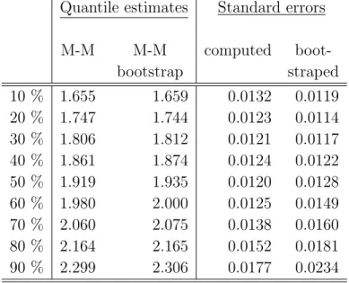
Machado and Mata (2005) use a bootstrap procedure to estimate standard errors for the quantiles of the counterfactual distribution. So far as we know, no proof of the consistency of this procedure has been given in the M-M framework. In addition, bootstrapping can be computationally demanding in this setting. The result that we present in Theorem 2 therefore has three advantages relative to the existing literature on the M-M procedure; namely, (i) it provides a rigorous way to evaluate the precision of quantile-based decompositions, (ii) it offers a (relatively) computationally less demanding alternative to the bootstrap, and (iii) it shows that the use of the bootstrap is consistent in this setting (see, for example, Horowitz 2001, Theorem 2.2). Of course, it is useful to compare the estimated asymptotic standard errors that can be computed using Theorem 2 with the corresponding bootstrap estimates. We do this in Appendix B in the context of the application that we present in Section 4. In general, the estimates generated by the two alternative procedures match well. More details are given in Section 4. We also note that our results in Theorems 1 and 2 refer to the pointwise limits in (0,1) of the quantile process. The same is true of the bootstrap procedure used in Machado and Mata (2005).
In our application, we are interested in log wage gaps, i.e., differences between quantiles of two log wage distributions. The quantiles of the distributions of YA
4
Melly (2007) proves consistency and asymptotic normality for the case in which the pop-ulation B regression quantiles are estimated using a grid and the entire sample of observables from population A is used in Step 3.
and YAB are correlated. The covariance between a particular quantile of these
two distributions can be shown to be equal to
q(1−q)
fYA(θ(q))fYAB(θ(q))
.
This results in a reduction in the variance of the log wage gap at theqth quantile.
The reduction does not arise when we consider differences in quantiles of the distributionsYB and YAB.5
3
Machado - Mata Decompositions with Sample
Selection Adjustment
In this section, we extend the M-M procedure to allow for selection.6 In our
application, we consider the selection of women into full-time work, so we explain our selection adjustment procedure in those terms. In the notation of the previous section, groupsA and B could stand for any arbitrary groups so, for example,A
could be women and B could be men. When we adjust for selection of women into full-time work, however, we letAdenote all women andB denote the women who actually work full time.
5
The intuition is as follows. The conditional quantiles ofYA given xA are given by YA =
xAβA(u) for u ∈ [0,1], while those of YAB given xA are given by YAB = xAβB(u) for u ∈
[0,1]. We can use the M-M method to recover the unconditional distributions of bothYA and
YAB. The sample from XA is used in constructing both distributions. This means that the
correlation between the two generated stochastic variables is essentially that betweenXAβbA(u)
andXAβbB(u).The correlation betweenYB andYAB does not have this feature because in that
case, we generateYB andYAB by sampling fromXB andXA,respectively. Note that a similar
correlation arises in the Oaxaca decomposition method. Details are available from the authors on request.
6
Considerable attention has been devoted to sample selection in the literature. Much of this work extends Heckman’s (1979) classic model to allow for non-normality. See, e.g., Gallant and Nychka (1998), Newey (1988), Das, Newey and Vella (2003), or Vella (1998) for a survey. There are other techniques we could have used to correct for sample selection across the distribution. For example, Blundell, Gosling, Ichimura and Meghir (2007) use the approach suggested in Manski (1994) to bound the possible impact of selection. The idea is simple: even if we know nothing about the productivity of non-workers, bounds can be obtained by assuming either that all non-workers are more productive than workers (resulting in the upper bound) or that all non-workers are less productive than workers (resulting in the lower bound). In contrast to Blundell et al., our objective is to construct point estimates of a counterfactual distribution. This, of course, implies that we need to make much stronger identifying assumptions than they do.
We thus let YA be the counterfactual random variable representing the log
wage that a randomly selected woman would earn were she to work full time. The quantiles of YA conditional on xA are given by
Quantu(YA|XA =xA) =xAβA(u) u∈[0,1],
whereβA(u) is the true value of the coefficient correcting for selection. We follow
Buchinsky (1998a) by estimating
Quantu(YB|ZB =zB) =xBβA(u) +hu(zBγ) u∈[0,1].
The stochastic vector Z is the set of observable characteristics that influence the probability that a woman works full time. In our application, these include the observables that influence her wage for full time work, i.e., the X′s, but for
identification, Z must also contain at least one variable that is not included in
X. This variable (or variables) should, of course, be uncorrelated with the log wage. Note that whereas zA is a draw from the distribution of covariates among
all women,zB is a draw from the distribution of the same covariates but now only
among those women who work full time. That is, we can only estimate βA(u)
using observations on the women who actually work full time.
The term hu(zBγ) corrects for selection at the uth quantile. It plays the
role that the Mill’s ratio plays in the usual Heckman (1979) procedure, but it is quantile-specific and more general so as not to assume normality. Note that we are making a single-index assumption. In doing so, we are directly following the argument given on pp. 3-5 in Buchinsky (1998a). This argument compares the market wage, i.e., the wage a woman would earn in full-time work, with her reser-vation wage. Of course, both the market wage and the reserreser-vation wage depend in part on unobservables. Buchinsky (1998a) gives conditions (his Assumptions C and E, p. 4) on the joint distribution of these unobservables, both uncondi-tionally and conditional onx,that justify the single-index representation.7 These
assumptions, while sufficient for the single-index representation, do not pin down the form of hu(·). Buchinsky (1998a) therefore suggests a series estimator (see
also Newey 1988), namely,
c
hu(zBγ) = δ0(u) +δ1(u)λ(zBγ) +δ2(u)λ(zBγ)2+. . . ,
where λ(·) is the inverse Mills ratio. The function chu(zBγ) is a power series
approximation ofhu(zBγ). For appropriate values of theδ’s,chu(zBγ)→hu(zBγ)
7
These assumptions are not uncontroversial. It seems difficult to specify a data-generating process that literally conforms to Assumptions C and E. The core objective, however, is to allow for a selection effect that varies across quantiles, and terms of the formhu(zBγ) can be
as the number of terms goes to infinity. Of course, the use of the inverse Mills ratio is not necessary. Any function of zBγ, the single index, could be used,
including the single index itself.
Two problems remain before we can present our extension of the M-M proce-dure to adjust for selection. First, we need to estimateγ. If we could regress the reservation wage on the observables, that would give a consistent estimate of γ. However, we only observe whether the difference between the market wage and the reservation wage is positive – in the usual notation of the selection literature, we only observe whether a dummy indicator D equals 1 or 0. We proceed by minimizing the squared distance between D and P(D = 1|Z =z) ≡ Ψ(zγ). As we do not know the form of this conditional probability, we estimate Ψ(·) using kernel regression. This semi-parametric least squares procedure, as described in Ichimura (1993), gives a consistent estimate of γ. Again, we are following the approach taken in Buchinsky (1998a).
Second, we need to take account of the fact that when estimating a semi-parametric sample selection model as described above, the intercept in the wage equation is not identified. The problem is one of distinguishing between the in-tercept, βA
0(u), that we want to estimate and the first term in the power series
approximation to the selection correction term, δ0(u). As in Buchinsky (1998a)
and Andrews and Schafgans (1998), βA
0 (u) can be estimated through an
identi-fication at infinity approach. That is, one chooses a subsample of observations with values of the observables such that the probability of full-time work given those values is arbitrarily close to one and then uses that subsample to estimate
βA
0(u) without adjusting for selection.
Our extension of the M-M algorithm to adjust for selection is as follows:
1. Estimate γ using a single-index method, e.g., Ichimura (1993).
2. Sample u from a standard uniform distribution.
3. Compute βbA(u) using the Buchinsky technique.
4. Sample xA from the empirical distribution GbXA.
5. Compute byA=xAβbA(u).
6. Repeat steps 2 - 5 M times.8
8
The simulation procedure given in Steps 2 - 6 is simply an application of Machado-Mata in a slightly nonstandard context. The fact that the estimates of βA(u) need to be corrected for selection introduces an extra difficulty. The only role that the Buchinsky (1998a) technique plays in our analysis is to overcome this problem. If another method to correct for selection
Following the above procedure simulates the distribution of women’s log wages that we would expect to observe if all women worked full time. The difference between this distribution and the distribution across women who actually work full time gives the effect of selection. Our procedure corrects both for selection on observables and for selection on unobservables. This can be understood as follows. We are simulating draws from
FYA(y) = Z
FYA(y|XA=x)dGXA(x).
We correct for selection on observables by accounting for the fact that the distri-bution of observables across all women is not the same as the one across women who work full time. We correct for selection on unobservables by accounting for the fact that the conditional distribution of log wages given observables is not the same as the one across women who work full time. Equivalently, given that these conditional distributions are completely characterized by{βA(u) :u
∈[0,1]}and
{βB(u) : u
∈ [0,1]} respectively, we correct for selection on unobservables by accounting for the difference between the selection-corrected and the uncorrected quantile regression coefficients.
In fact, we can decompose the overall selection effect into a part due to observ-ables and a part due to unobservobserv-ables. To do this, we construct another hypo-thetical distribution by modifying step 4 and sampling from the data on women who work full time. We then obtain the distribution that would result if women who do not work full time had the same distribution of observed characteristics as those who do work full time. The difference between these two distributions is the portion of the selection effect due to observed characteristics. The remain-der of the sample selection effect is the part due to unobserved characteristics. This latter portion can be obtained by comparing the distribution obtained by sampling from full-time working women with the original distribution of observed women’s wages.
4
Application: Log Wage Gender Gap in the
Netherlands
In this section, we use the M-M technique to analyze the gender gap across the log wage distribution for men and women who work full time in the Netherlands.
in quantile regression were available, that alternative technique could be used in Step 3. In all other respects, the logic underlying our use of Machado-Mata to correct for selection would be the same.
Studies of other European countries have found significant differences in the gen-der gap at different quantiles of the log wage distribution.9 As in Sweden and
Denmark, but unlike, for example, Switzerland, we find a glass ceiling effect in the Netherlands. That is, comparing the distributions of log wages of men and women who work full time, the gender gap is greatest at the highest quantiles, although this effect is not as pronounced as in the Scandinavian countries. As a first step to understand this pattern, we use the M-M method without correcting for selection and as in Albrecht, Bj¨orklund, and Vroman (2003), we decompose the difference between the male and female full-time log wage distributions into a component due to the difference in the distributions of observable characteristics between genders and a component due to the difference in the distributions of rewards to these characteristics between genders. As in the Swedish case, most of the difference between the two log wage distributions remains after we control for the difference between the male and female distributions of characteristics.
This, however, ignores an important part of the story. As noted in the intro-duction, part-time work is common among women in the Netherlands, so sample selection is a serious issue.10 Consequently, we use our extension of the M-M
tech-nique to adjust for this selection and construct a counterfactual distribution of full-time log wages for women, namely, the distribution that would have prevailed had all women worked full time. The overall selection effect is strongly positive; that is, the women who actually work full time are those with the highest poten-tial wages. Had all women worked full time in the Netherlands, the gender gap
9
See Albrecht, Bj¨orklund and Vroman (2003) for Sweden, Blundell, Gosling, Ichimura and Meghir (2007) for the UK, Bonjour and Gerfin (2001) for Switzerland, Datta Gupta, Oaxaca and Smith (2006) for Denmark, de la Rica, Dolado and Llorens (2008) for Spain, Fitzenberger and Wunderlich (2002) for Germany, and Arulampalam, Booth and Bryan (2007) for several European countries.
10
In terms of gender, the Dutch labor market has changed dramatically over the past 20 years. In 1980, the gender gap in employment was about 40%, similar to that of Spain, Greece, Italy, and Ireland. By 2000, this gap had fallen to a level (about 18%) more like that of most other Western European countries, albeit still above the levels observed in the U.S., the U.K., and the Scandinavian countries. Most of this change was due to an expansion of part-time work for women. In 2000, the Netherlands had the highest rate of part-time work (defined as fewer than 30 hours per week) among women in all the OECD countries. About 56% of employment among women aged 25-54 was part time. This is considerably higher than the corresponding rates for Germany and Belgium (35%), France (23%), the U.K. (38%) and the U.S. (14%). Only Switzerland (47%) is remotely comparable. This difference relative to other countries was mainly caused by high part-time employment rates for mothers. For example, 83% of working mothers aged 25-54 with 2 or more children worked part time. The comparable figure for the U.S. is 24%. The part-time employment rate of men in the same age group in the Netherlands (6%) is not substantially different from other countries, especially when we look at fathers. These figures are taken from the July 2002 OECD Economic Outlook.
would have been considerably larger. Our technique also allows us to decompose the selection effect into a portion due to observables and a portion due to unob-servables. Most of the selection effect is explained by obunob-servables. Finally, we use the M-M technique to construct a counterfactual to the counterfactual, namely, the distribution of log wages that women would earn if all women worked full time and had the male distribution of labor market characteristics.
4.1
Data
We use data from the OSA (Dutch Institute for Labor Studies) Labor Supply Panel. This panel dates from 1985 and is based on biannual (1986, 1988, etc.) interviews of a representative sample of about 2,000 households. All members of these households between the ages of 16 and 65 who were not in (daytime) school and who could potentially work were interviewed. The survey focuses on respondents’ labor market experiences. Van den Berg and Ridder (1998) give a detailed description.11 We use data from the 1992 survey for all of our analysis.
This year is particularly rich in terms of variables that can be used to explain participation in full-time work.12 The sample size for 1992 is 4536. In order to
focus on those who are most likely to be working full time, i.e., on those who are least likely to still be in school or already retired, we restrict our sample to individuals between 25 and 55 years of age inclusive. We deleted 1238 individuals who fell outside this range. In addition, among those who were not working at the survey date, there are relatively many individuals with missing data for years of work experience. We set work experience equal to 0 for those who did not work in the previous 2 years. All others lacking experience data were dropped from our dataset. This led to an additional 113 deletions. This leaves a sample of 1617 females and 1568 males. Of course, not all of these individuals worked full time. In terms of full-time wage data, we deleted observations lacking a reported wage. These include 1463 individuals who did not work full-time plus 94 nonresponses. We also deleted two individuals reporting wages below 2 euros or exceeding 20 euros per hour.13 Finally, we deleted two individuals who reported contractual
hours per week above 60 hours, as this is likely to be due to measurement error. This leaves 391 women and 1233 men who reported usable full-time wages. We
11
A description can also be found at http://www.uvt.nl/osa.
12
We have repeated our analysis using data from the 1998 survey and have found qualitatively similar results. We prefer to use the 1992 data because they are better suited for dealing with the selection issue.
13
The minimum wage in the Netherlands was the equivalent of 983 Euros per month for a full-time worker over 22 years of age. This implies a gross wage of about 5.5 Euros per hour. The reported wages are net wages, but this cannot explain wages below 2 Euros per hour.
use the data on all 1617 women to carry out the selection analysis.
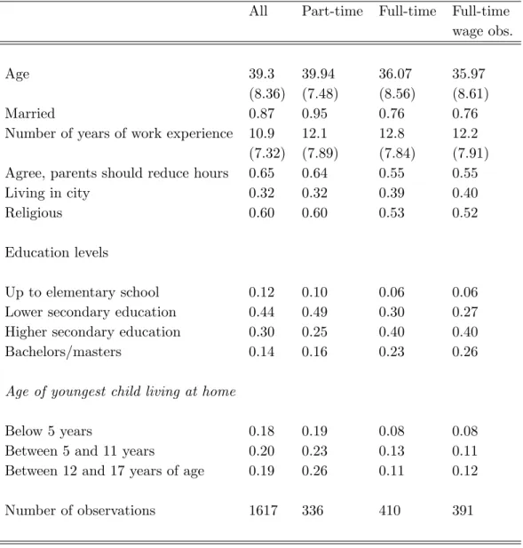
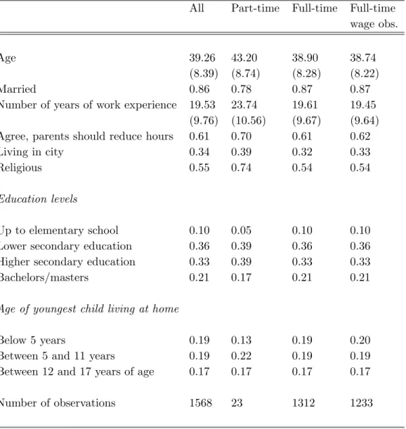
In Table 1, we give some descriptive statistics for the key variables for all women, women working part time, women working full time and women working full time with reported wages. Similar descriptive statistics for men are presented in Table 2 (likewise for all men, men working part time, men working full time and men working full time with reported wages). Most men between the ages of 25 and 55 work, and among those who are working, almost all work full time. Among women, the situation is quite different. In terms of the variables that we can use to explain variation in wages, there are also some important differences between the genders. Among those working full time and reporting wages, men are on average almost 3 years older than women, and years of work experience are much higher for men than for women. We measure education using four categories – (i) up to elementary education, (ii) lower secondary education, (iii) upper secondary education, and (iv) bachelors/masters degree.14 Overall, men
have achieved higher levels of education than women have, but if we compare men and women who work full time, this pattern is reversed. In general, women are slightly more likely to be married than men are. This is simply because women tend to marry men who are older than they are. However, women who work part time are much more likely to be married than are women in general, and women who work full time are much less likely to be married. Finally, men and women are approximately equally likely to live in cities, but women who work full time are much more likely to do so than are men who work full time.
The data include variables concerning attitudes about working and about the relationship between family and work.15 We use reactions to the statement,
“Parents should be willing to reduce working hours for childcare.” Respondents could reply that they completely disagreed, disagreed, were indifferent, agreed or completely agreed. We count those individuals who either agreed or completely agreed as agreeing with the statement. Women who work full time are less likely to agree with this statement than are other women. We also have data on whether there are children in the household. We report whether there are children living at home and whether the youngest child is (i) below 5 years of age, (ii) age 5-11, or (iii) age 12-17. Relatively few women who are working full time have children living at home (32%); relatively many women working part time do. This phenomenon is even more apparent when we look at the youngest age group. Only 8 percent of the full-time working women who report wages have
14
Our education variable is based on the first digit of the ISCED codes. Lower secondary education is level 3, upper secondary education is level 4 and our last category includes all education levels exceeding level 4.
15
children below the age of 5 living at home, while among all women in the sample, this figure is 18 percent. The same holds true for children 5-11 and 12-17, but the percentage differences are smaller. Finally, we have a variable that summarizes religious attitudes. Overall, women seem to be a bit more “religious” than men, but this difference disappears when we compare full-time workers among men and women.
In sum, full-time working women are more educated, less likely to be married, less likely to have (young) children at home, and have different attitudes towards working than women who do not work full time.
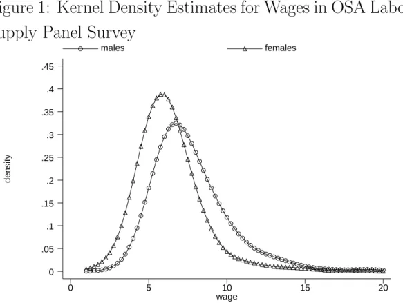
Table 3 gives wages for women who work part time, for women who work full time, and for men. These are net hourly wages excluding extra payments for overtime, shift work, bonuses, tips etc. As expected, men’s wages are on average higher than women’s wages. The average wage among women working full time is slightly higher than the corresponding average among women who work part time.
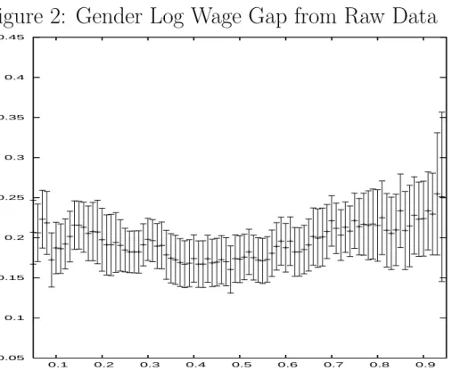
Figure 1 plots the estimated kernel densities of men’s and women’s wages. In this figure, we use all wages, including those of part-time workers. The gender gap, i.e., the difference in log wages between males and females at each quantile of their respective distributions, is plotted in Figure 2. This figure shows the gap for all working men versus all working women, i.e., both the male and female distributions include part-time workers. We show the 95% confidence bands in Figure 2. The variance used in the calculation of the confidence interval for difference in the qth quantiles is estimated using q(1−q)
b fA(θb(q))2 + q(1−q) b fB(bθ(q))2 , where b
θ(q) is our estimate of the qth quantile and the densities f
A(·) and fB(·) are
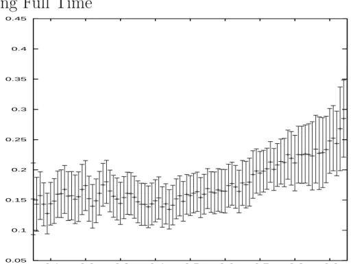
estimated using a kernel density method. Figure 3 shows the corresponding gap for men versus full-time women. Figures 2 and 3 show different patterns for the gender gap across the distribution. In Figure 2, the gender gap is relatively flat, but in Figure 3, the gender gap is larger at higher quantiles. That is, the gender gap between men and women who work full time exhibits a glass ceiling effect; full-time working women do relatively well at the bottom of the wage distribution but not as well at the top. This pattern is presented in a different form in Figure 4, which plots the gap between the log wages of women who work full time and those who work part time. We focus on the pattern in Figure 3. That is, we focus on men versus women who work full time.
4.2
Single-Index Estimation and Quantile Regressions
We begin by estimating log wage quantile regressions for women and for men who work full time. We regress log wage on the basic human capital variables, years of work experience and education (with less than secondary education as the left out category), as well as marital status and whether the individual lived in a city. However, in comparing the quantile regressions for men and women, we need to account for the selection of women into full-time work. As described above, we use the method introduced by Buchinsky (1998a) to correct for selection in quantile regression. We make this adjustment only for women.
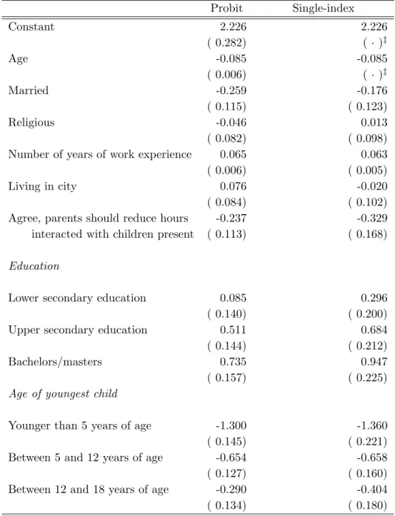
Table 4 presents our estimates of the determinants of full-time work among women.16 The first column gives probit results, while the second column contains
the results for an estimation using the Ichimura (1993) single-index technique.17
Table 4 indicates that older and married women are less likely to work full time. Highly educated women are more likely to work full time, as are women with a relatively high level of work experience. Having a young child at home has a strong negative impact on the propensity to work full time and is more important the lower the age of the youngest child. Finally, women with children who respond that it is better for women to stay at home when they have children are less likely to work full time. Whether or not a woman lives in a city seems to have little impact on the incidence of full-time work nor does the religion variable.
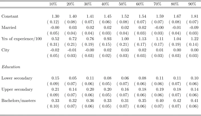
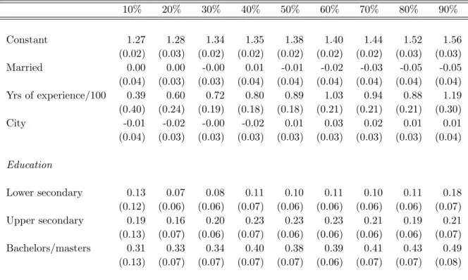
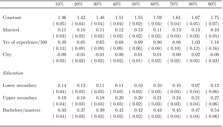
Table 5 presents the uncorrected quantile regressions results for full-time work-ing women, while Table 6 presents the correspondwork-ing results with the Buchinsky correction.18 The quantile regression results for men are in Table 7. In the
un-corrected estimates for women, the basic human capital variables are the most important and have the anticipated effects. That is, work experience has a pos-itive effect, which rises across the quantiles, and education has a strong pospos-itive effect. Marital status and the dummy for living in a city have insignificant effects at almost all the quantiles. Correcting for selection has several effects. First,
16
We model full-time work as a matter of choice for women. We base this on our comparison of histograms for desired versus contractual working hours for both men and women (not shown). In fact, the match between desired and contractual hours is much closer for women than for men.
17
Note that the constant and the coefficient of one of the continuous variables are not iden-tified in a single-index model. Hence, we normalize by setting the constant and the coefficient on age equal to their values in the probit model so that the probit and single-index results are comparable.
18
To implement the identification at infinity approach, we used a subsample of women, namely, those who are young, not married, highly educated (with a bachelors or masters de-gree), have no children, are not religious, live in the city and do not agree with the statement that parents should reduce working hours to care for their children.
the estimated constant terms decrease once we adjust for selection, especially towards the top of the distribution. Second, the rewards to education increase in the upper part of the distribution after correcting for selection. Table 7 indicates that men also receive a positive return to education. As is the case for women, the coefficients on years of experience are strongly positive and increase across the distribution. Finally, the data show a strong marriage premium for men in the Netherlands, which is relatively constant across the distribution.
4.3
Decomposition Results without Selection Correction
Next we turn to the decompositions. We first present a decomposition of the gender gap without correcting for selection. The results over the whole distribu-tion are best viewed graphically. For reference, recall that Figure 3 presented the gender log wage gap for men versus women working full time based on the raw data. This was derived by simply subtracting the log wage of the full-time women at each quantile of their log wage distribution from the log wage of the men at the corresponding quantiles of the male log wage distribution. As noted above, without conditioning on covariates or adjusting for selection, there is a significant glass ceiling effect in the data, i.e., the gender gap is significantly higher at the higher quantiles of the distribution. We now use the M-M procedure to analyze what proportion of the gap is due to differences in labor market characteristics between the genders and what proportion is due to differences in the returns to these characteristics between the genders.
Figure 5 plots the wage gap that remains after we take into account the differ-ence in distributions of observed characteristics between men and women. That is, we construct a counterfactual distribution using the M-M method that gives the log wage distribution that women would have earned if they had the same distribution of characteristics as men but were still paid for those characteristics like women. The characteristics that we include are those given in the quantile regression tables, namely, experience, education, marital status, and whether the individual lived in a city.19 As can be seen in Figure 5, a significant positive
gender gap across the whole distribution remains. Comparing Figure 5 to Figure 3, we can see that at the bottom of the distribution, only a small part of the gender gap for full-time workers is due to differences in characteristics between men and women. Above the median, approximately one third of the gap can be explained in this way.
19
The standard errors underlying the confidence bands in Figure 5 are computed using the expression given in Theorem 2. Appendix B compares the M-M quantile estimate and standard errors with the corresponding bootstrap estimates. The two sets of estimates match quite well.
To confirm that most of the gender gap is due to differences in returns to characteristics, we also construct a counterfactual distribution of log wages that represents the wages that women who work full time would earn if they retained their observed characteristics but were paid for them like men. The gap between the log wages of men and the log wages given in this counterfactual distribution is presented in Figure 6. The gap is smaller over the whole distribution. Figures 5 and 6 show that most of the gender log wage gap between men and women who work full time is explained by differences in the returns to observed characteristics between the genders as opposed to differences in these characteristics.
We note that the standard errors presented in Figures 5 and 6 are computed using the expression for the variance of the limiting distribution of θb(q) that is given in Theorem 2. The standard errors in these two figures are standard errors for differences between the quantiles of two distributions, and as noted in Section 2, there is a positive covariance between the quantiles ofYA and those of YAB.
4.4
Decomposition Results with Selection Correction
We next investigate the effect of sample selection on the women’s log wage distri-bution and on the counterfactual distridistri-bution. To see the direct effect of selection, we first look at the gap between the log wage distribution for women working full time and the log wage distribution that we would have observed had all women worked full time. Figure 7 shows that the overall selection effect is positive. That is, women who actually work full time have higher earnings potential in full-time work than do women in general. This difference is significantly positive across almost all of the distribution.
In Figure 8, we show the gender log wage gap after adjusting for selection, i.e., we plot the difference between the male log wage distribution and the log wage distribution for women that we would expect to observe if all women worked full time. This can be compared with the gender log wage gap in the raw data shown in Figure 3. This gap after adjustment for selection is significantly greater at almost all quantiles.
The results taking the selection effects into account are based on sampling characteristics from the data set for all women. In Step 4 of our modification of the M-M procedure to deal with selection, if we had only sampled women working full time, we would have ignored the impact of the difference between the observed characteristics of women who do and do not work full time. Al-though this would have resulted in the wrong distribution and hence the wrong wage gaps, it is a useful exercise in order to explain the sample selection effect. This distribution can be interpreted as the distribution of wages that would have
resulted if the women who do not work full time had the same characteristics as those who do work full time. Hence, comparing the distribution with the proper sample selection correction with this distribution allows us to view the portion of the selection effect due to observed characteristics. The remainder of the sample selection effect is the part due to unobserved characteristics. The portion due to the unobserved characteristics can be obtained by comparing the distribution obtained from sampling from full-time working women with the original distri-bution of observed women’s wages. Figures 9 and 10 present the observed and unobserved parts of the selection effect. The observed part is positive across the distribution, reflecting the fact that women who work full time are in general bet-ter educated and have more work experience than women who are not working full time. The unobserved part of the sample selection effect is also positive across the distribution. In general, observables account for most of the selection effect. For example, at the median, observables account for more than three quarters of the sample selection bias.
Finally, we can address the issue of what proportion of the wage gap shown in Figure 8, that is, the gap between men and women that we would observe if all women worked full time, is due to differences in characteristics between men and women and what proportion is due to differences in returns to these characteristics between the genders. Figure 11 shows the difference between the male log wage distribution and the distribution of log wages that women would earn if all women worked full time and had the characteristics of men but received the returns of women (adjusted for sample selection). As can be seen from the figure, accounting for the difference in characteristics reduces the gender gap by a bit less than one third on average with the greatest effect in the middle of the distribution.
Concluding, we find a positive and significant selection effect for full-time work in the Netherlands. A large part of the selection effect is due to observables. Compared with the decomposition results presented in Section 4.3, accounting for differences in observables between men and all women, including those who do not work full time, has more of an impact on the gender log wage gap, espe-cially toward the bottom of the distribution. This result reflects the fact that, in contrast to what we observe in the population of women working full time, education and years of work experience in the population of all women are lower than the corresponding levels for males.
5
Conclusions
In this paper, we have made three contributions. First, we have contributed to the econometrics underlying the M-M quantile regression decomposition technique. This method is an intuitively appealing generalization of the Oaxaca-Blinder ap-proach, which decomposes differences between groups in average outcomes into differences in average characteristics and differences in rewards to those charac-teristics. The M-M method is designed to simulate counterfactual distributions; for example, what would the distribution of full-time log wages for women have been if working women had the same distribution of labor market characteristics as men do? We have shown that the M-M method leads to consistent estimators for the quantiles of the counterfactual distribution that it is designed to simulate, and we have developed asymptotic standard errors for these estimators. Second, we have extended the M-M technique to account for selection. The idea is to use the technique to simulate another counterfactual distribution; for example, the distribution of full-time log wages for women if all women worked full time. Our method for accounting for selection also allows us to decompose the selection effect into a component due to observables and one due to unobservables.
Our third contribution has been to apply our extension of the M-M technique to help understand the gender gap in the Netherlands. Specifically, we examined the difference between the male and female distributions of log wages among full-time workers. Taking the population of women working full full-time as given, we found an average log wage gap on the order of 15-20%, and we documented that this gap increases as we move up the distribution. That is, a glass ceiling effect is present in the Netherlands. However, relatively many women work part time in the Netherlands, so the sample of women working full time is a selected one. We addressed several questions in connection with this selection process. First, what would the difference between the male and female log wage distributions among full-time workers have looked like if all women had worked full time? In fact, correcting for selection turns out to be very important. Were all Dutch women to work full time, the average log wage gap between the genders would be much higher; that is, there is a strong positive selection into full-time work among women in the Netherlands. Second, how can we explain the selection we observe? Our technique allows us to ascribe most of the selection effect to observables – women who are working full time have higher education and more work experience than other women do. Finally, if we compare the distribution of log wages that we would observe if women worked full time with the correspond-ing distribution across men, to what extent would the difference between the counterfactual female distribution and the actual male distribution be ascribed
to differences in characteristics? We found that a bit less than one third of this counterfactual difference would be ascribed to differences in the distributions of characteristics between men and women. That is, once we correct for selection, differences in labor market characteristics between men and women play a larger role in explaining the gender gap in the Netherlands. Nonetheless, most of the gender gap across the distribution continues to be accounted for by differences in how men and women are rewarded.
References
Albrecht, J., A. Bj¨orklund and S. Vroman (2003), Is there a glass ceiling in Sweden?,
Journal of Labor Economics, 21, 145–177.
Andrews D.W. and M.A. Schafgans (1998), Semiparametric estimation of the intercept model,Review of Economic Studies, 65, 497–517.
Arulampalam, W., A. Booth, and M. Bryan (2007), Is there a glass ceiling over Europe? Exploring the gender pay gap across the wages distribution,Industrial
and Labor Relations Review,60, 163-186.
Autor, D.H., L.F. Katz, and M.S. Kearney (2005), Rising wage inequality: The role of composition and prices,NBER working paper 11628
Blundell, R., A. Gosling, H. Ichimura and C. Meghir (2007), Changes in the distri-bution of male and female wages accounting for employment composition using bounds,Econometrica, 75, 323-364.
Bonjour, D. and M. Gerfin (2001), The unequal distribution of unequal pay - an empirical analysis of the gender wage gap in Switzerland,Empirical Economics, 26, 407–427.
Buchinsky, M. (1998a), The dynamics of changes in the female wage distribution in the USA: a quantile regression approach, Journal of Applied Econometrics, 13, 1–30.
Buchinsky, M. (1998b), Recent advances in quantile regression models: a practical guideline for empirical research,Journal of Human Resources, 33, 88-126. Das, M., W.K. Newey and F. Vella (2003), Nonparametric estimation of sample
se-lection models,Review of Economic Studies, 70, 33–58.
Datta Gupta, N., R. Oaxaca, and N. Smith (2006), Swimming upstream, floating downstream: Trends in the U.S. and Danish gender wage gaps, Industrial and
Labor Relations Review,59, 243-266.
de la Rica, S., Dolado, J. and V. Llorens (2008), Ceilings or floors? Gender wage gaps by education in Spain,Journal of Population Economics, 21, 751-776.
Dinardo, J., N.M. Fortin and T. Lemieux (1996), Labor market institutions and the distribution of wages 1973-1992: a semiparametric approach, Econometrica, 64, 1001-1024.
Donald, S., D. Green, and H. Paarsch (2000), Differences in wage distributions be-tween Canada and the United States: An application of a flexible estimator of distributions in the presence of covariates, Review of Economic Studies, 67, 609-633.
Fitzenberger, B. and G. Wunderlich (2002), Gender wage differences in West Ger-many: a cohort analysis,German Economic Review, 3, 379–414.
Gallant, A.R. and D.W. Nychka (1987), Semi-Parametric Maximum Likelihood Esti-mation,Econometrica, 55, 363-390.
Heckman, J. (1979), Sample Selection Bias as a Specifcation Error,Econometrica, 47, 153-161.
Horowitz, J. (2001), The Bootstrap, in: J.J. Heckman and E.E. Leamer,Handbook of
Econometrics, 5, Elsevier B.V.
Ichimura, H. (1993), Semiparametric least squares (SLS) and weighted SLS estimation of single index models,Journal of Econometrics, 58, 71–120.
Koenker, R. and G. Bassett (1978), Regression Quantiles,Econometrica, 46, 33-50. Law, A.M. and W.D. Kelton (1991),Simulation modelling and analysis, McGraw-Hill,
New York.
Lemieux, T. (2002), Decomposing differences in distributions; A unified approach,
Canadian Journal of Economics, 35, 646-688.
Machado, J.A.F. and J. Mata (2005), Counterfactual decomposition of changes in wage distributions using quantile regression, Journal of Applied Econometrics, 20, 445-65.
Manski, C. (1994), The selection problem, in C. Sims, Advances in Econometrics,
Sixth World Congress, 1, Cambridge University Press.
Melly, B. (2007), Estimation of Counterfactual Distributions Using Quantile Regres-sion, mimeo.
Newey, W.K. (1988), Two step series estimation of sample selection models, working paper, Cambridge.
Newey, W.K. and D. McFadden (1994), Large Sample Estimation and Hypothesis Testing, in R.H. Engle and D. McFadden (eds.), Handbook of Econometrics,
Oaxaca, R. (1973), Male-Female Differentials in Urban Labor Markets, International
Economic Review, 14, 693-709.
OECD (2002), Employment Outlook 2002, OECD, Paris.
Silverman, B.W. (1986), Density estimation, Chapman and Hall, London.
Van den Berg, G.J. and G. Ridder (1998), An empirical equilibrium search model of the labor market,Econometrica, 66, 153–161.
Van der Vaart, A. (1998), Asymptotic statistics, Cambridge University Press, Cam-bridge.
Vella, F. (1998), Estimating models of sample selection bias, Journal of Human
Re-courses, 61, 191–211.
Appendix
A
Theorems and Proofs
A.1
Consistency and Asymptotic Normality
We make the following assumptions about the distributions ofYB, XA,and XB:
Assumptions A
A1. FYBhas a compact support on R and is continuously differentiable on its
support with positive densityfYB
A2. GXAand GXBhave a compact support on R
K
A3. NB−1XBTXB converges in probability to a positive definite matrix
A4. ∀u∈[0,1] andxA∈supp(XA) : dxAβ
B(u)
du >0
A5. XA⊥XB
These assumptions ensure that the coefficient estimates that result from quan-tile regressions of YB on XB are consistent and asymptotically normal (see, for
example, Van der Vaart 1998, page 307 and Koenker and Bassett 1978). In addi-tion, the joint compactness assumption (together with Condition 4) guarantees that the support of FYAB is also a convex and compact subset of R (not proven
here).20 This is necessary to prove consistency and asymptotic normality ofbθ(q).
20
The conditions are somewhat stronger than strictly necessary. Identification may still be satisfied even if the support ofYAB is not a convex compact subset of R. Details about this
Assumption A.4 states that the quantile regression lines cannot cross on the sup-port of XA. Assumption A.5 is made for convenience and is only necessary for
the computation of the covariance. We make this assumption in order to satisfy the condition that the moments of the different subsamples of populationsAand
B are uncorrelated (for more details, see section 6.2 of Newey and McFadden, 1994).
When we correct for sample selection, Assumption A5 cannot hold because population B is a subset of population A. As noted above, Assumption A5 is only used in the case without selection for computing covariances between different regression quantiles. We do not use this assumption when we correct for sample selection – instead, we use the method presented in Buchinsky (1998a).
In addition, when we correct for sample selection, an extra assumption is needed to ensure that the quantile regression estimators are consistent and asymp-totically normal, namely,
Assumption A5′: Quantu(YB−xBβA(u)−hu(zBγ)|ZB=zB) = 0 u∈[0,1].
Assumption A5′ is necessary to estimate βA(u) consistently. Thus, this
assump-tion is necessary for consistency when adjusting for selecassump-tion (unlike Assumpassump-tion A5 in Theorem 1). Assumption A5′ was also made by Buchinsky (1998a).
Theorem 1 Let Assumptions A1-A4 be satisfied, and let M, NA, NB → ∞ with M/NA →IA<∞, M/NB →IB <∞. Then θb(q)
p
→θ0(q).
The most important step in the proof is relatively simple and is based on the in-verse transformation method (see, for example, Law and Kelton 1991). However, this method assumes that the underlying population distributions are known. In the M-M approach, these distributions are estimated. Hence, most of our proof is devoted to showing that when the sample sizes of both datasets are large, the impact of the estimation method is negligible.
In addition to consistency, it is important to prove asymptotic normality.
Theorem 2 Let Assumptions A1-A5 be satisfied, and let M, NA, NB → ∞ with M/NA →IA<∞, M/NB →IB <∞. Then √ M(θb(q)−θ0(q)) N(0,Ω) with Ω = IAq(1−q) +IBEXA,U,V f2 YAB(θ(q)|XA =xA)X T AΛ(βB(U), βB(V))XA f2 YAB(θ(q))
and Λ(βB(u), βB(v)), u, v ∈[0,1]given by Λ(βB(u), βB(v)) = EXB fYB(XBβ B(u))X BXBT −1 u(1−v)EXB(XBX T B) ×EXB fYB(XBβ B(u))X BXBT −1 if u≤v EXB fYB(XBβ B(u))X BXBT −1 v(1−u)EXB(XBX T B) ×EXB fYB(XBβ B(u))X BXBT −1 otherwise
where U and V are independent standard uniform random variables.
Before proving these theorems, we have four comments about Theorem 2. The first comment is about the two terms in the numerator of Ω. The first term is the standard deviation of the estimated quantile atq based on a sample of size NA.
Indeed if IB →0, the variance converges to this term since in that case the only
randomness comes from theXA’s. The second term, which is quite complicated,
takes into account the estimation of the βB(u)’s across the distribution. The
complexity of this term is mainly due to the fact that even though we sample independent draws from a uniform distribution, the resulting quantile regression estimates are not independent of each other.
Second, the expression for Λ(βB(u), βB(v)), which is derived below in a
sep-arate lemma (see also Koenker and Bassett 1978, Theorem 4.2), is an extension of the usual expression for the covariance matrix for regression quantiles. This covariance matrix can be derived when u =v is substituted into the expression above. Whenuandv are different, the expression gives the covariance between re-gression quantiles at different points in the distribution. The expression is largest whenuand v are close to each other, and its maximum occurs whenu=v. This makes sense since ifu andv are close to each other, we are essentially comparing nearby quantiles, so the regression quantiles are likely to be close to each other as well. When u and v are far apart, the regression quantile βB(u) gives little
information aboutβB(v). In that case, the covariance between the two regression
quantiles is low.
Third, in terms of implementing our procedure, we use a kernel density method to estimate the covariance matrix Λ(·) (see Buchinsky 1998b). In ad-dition, we use the following estimates to complete the calculation of Ω:
b IA= M NA b IB= M N
b EXA,U,V fY2AB(θ(q)|XA=xA)XAΛ(β B (U), βB(V))XAT = " 1 M hM M X i=1 K θ(q)−yABi hM xAi #T " 1 M2 M X i=1 M X j=1 b Λ(βB(u i), βB(uj)) # × " 1 M hM M X i=1 K θ(q)−yABi hM xAi # b Λ(βB(u i), βB(uj)) = " 1 M hM M X l=1 K yBl−xBlβb B(u i) hM ! xBlx T Bi #−1 × " ui(1−uj) 1 M M X l=1 xBlx T Bl # " 1 M hM M X l=1 K yBl−xBlβb B(u j) hM ! xBix T Bi #−1 b fYAB(y) = 1 M hM M X l=1 K xAlβb B(u l)−y hM !
wherehM is the bandwidth andK is the kernel function.
Finally, when we correct for sample selection we can extend Theorem 2 by replacing Λ(·) by the covariance matrix that is computed using the Buchinsky (1998a) technique.
A.2
Proofs of Theorems 1 and 2
A.2.1 Proof of theorem 1We first consider the estimatorθe(q), which is the sample quantile obtained from the sampleyei;i= 1. . . M. This sample is obtained as follows
1. Sample ui from a standard uniform distribution
2. Sample xei from the distributionGXA
3. Compute eyi =exiβB(ui)
4. Repeat steps 1 to 3 M times.
The realizations of this method can itself be seen as realizations of a stochastic variable. Denote this variable byYeAB. The distribution function of this variable
is FYe AB(y) = Z 1 0 Z supp(XA) P(YeAB ≤y|U =u;XA=xA)dGXA(xA)du = Z 1 0 Z supp(XA) 1{xAβB(u)≤y}dGXA(xA)du = Z 1 0 Z supp(XA) 1n F−1 YAB(u|XA=xA)≤y odGX A(xA)du = Z supp(XA) Z FYAB(y|XA=xA) 0 dudGXA(xA) = Z supp(XA) FYAB(y|XA=xA)dGXA(x) =FYAB(y) (1) Hence,YeAB d
=YAB. This implies that the observations from the sampling method
are sampled from the population distribution YAB. For the remainder of this
proof we use vi as a k-dimensional vector that is used to sample from the
dis-tribution GXA and GbXA. The elements of vi are sampled from the standard
uni-form distribution.21 Hence Xe
A,i = XeA(vi) = GX−1A(vi) and likewise for XbA,i. Let
e
ΨM(θ(q)) = M1 Pimq(eyAB,i, θ(q)) and ΨbM(θ(q)) = M1 Pimq(byAB,i, θ(q), where
21
It is always possible to sample from a k-dimensional distribution with a known distribution function based on repetitive conditioning and a draw from a k-dimensional vector sampled from univariate uniform distributions. Although it is also possible to do this using the empirical distribution function of a k-dimensional stochastic vector, bootstrapping from the data would be a much easier way to obtain such a sample. For the remainder of the proof it does not matter.
m(yAB, θ(q)) = q(yAB−θ(q)) ifyAB > θ(q) (1−q)(θ(q)−yAB) ifyAB ≤θ(q) In addition, define Ψ(θ(q)) as Ψ(θ(q))≡ Z supp(YAB) m(yAB, θ(q))dFyAB(y) (2) = (1−q) Z θ(q) −∞ FyAB(y)dy+q Z ∞ θ(q) FyAB(y)dy
Taking derivatives, we obtain
Ψθ(q)(θ(q)) = (1−q)FyAB(θ(q)) +qFyAB(θ(q))
It can be easily checked that under assumption A-2 and A-4, this derivative has a single root. This is a sufficient condition for the identification for quantiles. It remains to show that
sup θ(q) bΨM(θ(q))−Ψ(θ(q)) =oP(1)
By the triangle inequality
sup θ(q) bΨM(θ(q))−Ψ(θ(q)) ≤sup θ(q) bΨM(θ(q))−ΨeM(θ(q)) + sup θ(q) eΨM(θ(q))−Ψ(θ(q)) (3)
The last term on the last line is oP(1) by the law of large numbers and the fact
thatYeAB
d
=YAB. It remains to show that the first term isoP(1) as well. We have
sup θ(q) bΨM(θ(q))−ΨeM(θ(q)) = sup θ(q) 1 M X b yi<θ q(ybi−θ(q))− 1 M X e yi<θ q(eyi−θ(q))+ 1 M X b yi≥θ (1−q)(θ(q)−ybi)− 1 M X e yi≥θ (1−q)(θ(q)−yei) ≤qsup θ(q) 1 M X e yi<θ(q) (ybi−eyi) + (1−q) supθ(q) 1 M X e yi≥θ(q) (yei−ybi) +qsup θ(q) 1 M X b yi<θ(q)≤yei (byi−θ(q)) +qsupθ(q) 1 M X e yi<θ(q)≤ybi (byi−θ(q)) + (1−q) sup θ(q) 1 M X b yi<θ(q)≤yei (θ(q)−ybi) + (1−q) sup θ(q) 1 M X e yi<θ(q)≤ybi (θ(q)−ybi) (4)
Making use of the definition ofybi,yei, bxi and xi and using the triangle inequality
again, we obtain (dropping superscriptB for β and A for x)
qsup θ(q) 1 M X e yi<θ(q) (ybi−yei) ≤supθ(q) 1 M X e yi<θ(q) b xi(vi) b β(ui)−β(ui) + 1 M X e yi<θ(q) b G−X1 A(vi)−G −1 XA(vi) β(ui) (5) We have that βb(ui) P
→ β(ui);i = 1, . . . M for NB → ∞ (uniform consistency of
quantile regressions on the open unit interval). Since M/NB → IB < ∞ when M, NB → ∞the first term isoP(1). For the second term, we have thatGb−X1A(vi)
P
→
G−X1A(vi) when n → ∞ due to a combination of the Glivenko-Cantelli theorem
(satisfied by A-2) and the continuous mapping theorem.22 Hence, the second
22
For the use of the continuous mapping theorem we need continuity of GXA(·). This is not an assumption in A1-A4. However, in case XA is strictly discrete
with mass xAj;j = 1, . . . l, then the second part of this equation changes into P
i
P
jxj(bpj−pj)β(ui), where thepbj’s andpj’s are the sample and population
frequen-cies of individuals with chararacteristics equal toxj. This term obviously converges to
zero in probability. Of course the most general case is whenXA contains both discrete
term in equation (5) is oP(1) as well (using M/NA →IA <∞ as M, NA → ∞).
This implies that the right-hand side of equation (5) and hence the first term on the right-hand side of equation (4) converges in probability to zero. The proof that the other terms on the right-hand side of (4) areop(1) as well is along
the same lines. Hence supθ(q)bΨM(θ(q))−ΨeM(θ(q))
converges in probability to zero when NA, NB → ∞. This implies that supθ(q)
bΨM(θ(q))−Ψ(θ(q)) (see equation (3)) converges to zero in probability since M/NA → IA < ∞. Using
theorem 5.7 of Van der Vaart (1998) completes the proof.
A.2.2 Proof of theorem 2
Before we are able to prove theorem 2 we need to prove the following lemma.
Lemma 3 Let q1, q2. . . qm ∈ (0,1), X be a k-dimensional random vector with
compact support onRk. In addition let β(q) be such that
Quantq(Y|X=x) =xβ(q)
where Y is a random variable with compact support on R. Then the regression quantiles βb(q1), . . .βb(qm) satisfy √ n b β(q1)−β(q1) .. . b β(qk)−β(qk) →N(0,Λ (β))
with Λ(β) an m×k by m×k dimensional matrix, where the elements of Λ(β)
are equal to Λ(β(qi), β(qj)) = EX fY(Xβ(qi))XXT −1 qi(1−qj)EX(XXT) ×EX fY(Xβ(qj))XXT −1 if i≤j EX fY(Xβ(qi))XXT −1 qj(1−qi)EX(XXT) ×EX fY(Xβ(qj))XXT −1 otherwise Proof
We drop the subscripts B in the proof. When we define ε = Y −Xβ then if
fε(·|X = x) = fε(·) the lemma is the same as theorem 4.2. of Koenker and
max β(q1),β(q2),...,β(qm) z(yi, β(q1), . . . , β(qm), q1, . . . , qm) where z(x, y, β(q1), . . . , β(qm), q1, . . . , qm) = m X i=1 qi(y−xβ(qi))1{y>xβ(qi)}+(1−qi)(xβ(qi)−y)1{y≤xβ(qi)} Define Ψ(β(q1), . . . , β(qm), q1, . . . , qm) = EY,X(z(X, Y, β(q1), . . . , β(qm), q1, . . . , qm))
It is possible to show that ∂Ψ
∂β(qi)
= EY,X[XFY(Xβ(qi))−xqi]
We denote the hessian of Ψ byH. Its elements are equal to (i.e. k×k matrices) Hij = ∂Ψ ∂β(qi)∂β(qj) = ( EY,X XXTf Y(Xβ(qi) ifi=j 0 otherwise
The first order derivative of z(x, y, β(q1), . . . , β(qm), q1, . . . , qm) with respect to β(qi) is equal to zβ(qi)(y, x, β(q1), . . . , β(qm), q1, . . . , qm) = −qix y > xβ(qi) (1−qi)x y ≤xβ(qi)
Hence the (expected) cross derivative matrix Z has the following elementsi, j = 1, . . . , m;j ≥i (i.e. k×k matrices) Zij = EY,X zβ(qi)zβT(q j) =qi(1−qj)EX(XXT)
The covariance matrix of√n(βb(q1)−β(q1), . . .βb(qm)−β(qm)) is equal to Λ(β) = H−1ZH−1. Taking the results above, the lemma follows immediately.
Proof of theorem 2: The criterion function to obtain bθ(q) is equal to
min θ(q) 1 M X b yABi>θ(q) qkbyABi −θk+ (1−q) X b yABi≤θ(q) kbyABi−θ(q)k= min θ M X i=1 m(byABi, θ(q))
where23 m(yAB, θ(q)) = q(yAB−θ(q)) ifyAB > θ(q) (1−q)(θ(q)−yAB) ifyAB ≤θ(q)
andybABi is the estimated level ofyABi (i.e. the i-th observation from the sample
using the M-M technique). The first order condition is equal to
M
X
i=1
∂m(ybABi,θb(q))
∂θ(q) = 0
In general we should take account of the fact that we are taking bootstrap samples fromXAand hence the convergence of the expression above is dependent on this.
As is proven in Van der Vaart (1998, page 333-334), this expression has the same limit as the statistic that results when we sample from the population instead of the data set. Hence we will not take this into account in the remainder of our analysis. Taking a first order Taylor series expansion of this results in
0 = √1 M M X i=1 ∂m(ybABi, θ(q)) ∂θ(q) + 1 M n X i=1 ∂2m(ybABi, θ(q)) ∂θ(q)2 √ M(θb(q)−θ(q)) +oP(1) (6)
We have that (see for example Van der Vaart (1998))
1 M n X i=1 ∂2m(yb ABi, θ(q)) ∂θ(q)2 P →fyABi(θ(q))
The first part on the right-hand side of equation (6) can be further expanded using a Taylor series expansion around the true value of theβ(u)′s
1 √ M M X i=1 ∂m(byABi, θ(q)) ∂θb(q) = 1 √ M M X i=1 ∂m(yABi, θ(q)) ∂θ(q) + r M NB 1 M M X i=1 ∂2m(yABi, θ(q)) ∂θ(q)∂βB(u i) p NB(βbB(ui)−βB(ui)) +oP(1) (7) 23
Note that the function presented is not differentiable everywhere. This is not necessary for the proofs presented below. In general it suffices to show that a Lipshitz condition holds. It is not difficult to show that this condition is satisfied. See Van der Vaart (1998) for more details.
Without loss of generality, we assume that the ui’s are in ascending order. The
second expression of equation (7) is non-standard because of the dependence between the regression quantiles. Using the analogy of equation (2) we obtain
EYAB(m(YAB, θ(q))) =q Z ∞ θ(q) F(y)dy+ (1−q) Z θ(q) −∞ F(y)dy =q Z 1 0 Z suppXA Z xAβB(u) θ(q) dy1{xAβB(u)>θ(q)}dGX A(xA)du + (1−q) Z 1 0 Z suppXA Z θ(q) xAβB(u) dy1{xAβB(u)≤θ(q)}dGXA(xA)du
In the second line we use equation (1) as well as a change of the integrals together with the observation that xAβB(u) > θ(q) whenever y > θ(q). The partial
derivative with respect to βB(u) is
EXA,U ∂m(YAB, θ(q)) ∂βB(U) =q Z 1 0 Z suppXA xA1{xAβB(u)>θ(q)}dGXA(xA)du −(1−q) Z 1 0 Z suppXA xA1{xAβB(u)≤θ(q)}dGXA(xA)du
Here we use the fact that limε↓0(1{θ(q)−ε<xAβB(u)≤θ(q)})/ε = 0 when we condition
on bothxAand u.The cross derivative with respect to θ(q) is
EXA,U ∂2m(YAB, θ(q)) ∂βB(U)∂θ(q) =−q Z 1 0 Z suppXA xAlim ε↓0 1 ε1{θ(q)<xAβB(u)≤θ(q)+ε}dGXA(xA)du −(1−q) Z 1 0 Z suppXA xAlim ε↓0 1 ε1{θ(q)<xAβB(u)≤θ(q)+ε}dGXA(xA)du =− Z 1 0 Z suppXA xAlim ε↓0 1 ε1{θ(q)<xAβB(u)≤θ(q)+ε}dGXA(xA)du =− Z suppXA xAfYAB(θ(q)|XA=xA)dGXA(xA) =−EXA(XAfYAB(θ(q)|XA=xA))
Combining this with lemma 3 we find that the second part of equation (7) con-verges to a 1 dimensional normal distribution with variance
<