Performance Comparison of Variational Mode Decomposition over Empirical Wavelet Transform for the Classification of Power Quality Disturbances Using Support Vector Machine

(1)

Procedia Computer Science 46 ( 2015 ) 372 – 380

Peer-review under responsibility of organizing committee of the International Conference on Information and Communication Technologies (ICICT 2014) doi: 10.1016/j.procs.2015.02.033

ScienceDirect

International Conference on Information and Communication Technologies (ICICT 2014)

Performance comparison of Variational Mode Decomposition over

Empirical Wavelet Transform for the classification of power quality

disturbances using Support Vector Machine

Aneesh C*, Sachin Kumar, Hisham P M, K P Soman

Centre for Excellence in Computational Engineering and Networking Amrita Vishwa Vidyapeetham,

Coimbatore Campus, Tamilnadu-641112.

Abstract

This work considers the classification of power quality disturbances based on VMD (Variational Mode Decomposition) and EWT (Empirical Wavelet Transform) using SVM (Support Vector Machine). Performance comparison of VMD over EWT is done for producing feature vectors that can extract salient and unique nature of these disturbances. In this paper, these two adaptive signal processing methods are used to produce three Intrinsic Mode Function (IMF) components of power quality signals. Feature vectors produced by finding sines and cosines of statistical parameter vector of three different IMF candidates are used for training SVM. Validation for six different classes of power qualities including normal sinusoidal signal, sag, swell, harmonics, sag with harmonics, swell with harmonics is performed using synthetic data in MATLAB. Classification results using SVM shows that VMD outperforms over EWT for feature extraction process and the classification accuracy is tabled.

Peer-review under responsibility of organizing committee of the International Conference on Information and Communication Technologies (ICICT 2014).

Keywords: Intrinsic mode function; Empirical wavelet transform; Empirical mode decomposition;Alternate direction method of multipliers; Variational mode decomposition; AM-FM signal

* Corresponding author. Tel.: 8754699468 E-mail address:[email protected]

Peer-review under responsibility of organizing committee of the International Conference on Information and Communication Technologies (ICICT 2014)

(2)

1.Introduction

Power quality signal detection and its classification is of great importance in industrial and commercial power system. The disturbances in power quality signal are threats for electronic equipments which are sensitive to these

disturbances1_{. Commonly these types of disturbances like swell, sag, harmonics are referred to as are referred to as}

the pollutions in power grid. The main sources include SMPS in computers, rectification circuits, non-linear resistive loads, inverters and verities of switching circuits, rotating machineries etc. Various techniques for detection and classification of power quality disturbances have been proposed recently. Mainly it includes hidden Markov

models2_{, artificial neural networks}3_{, Fourier and Wavelet transform for the analysis of harmonic pollution}4_etc.

Wavelet transform based processing of power quality disturbances is explained in5_{. There are rule based system for}

disturbance classification6_{in which decisions for classifications are performed using a set of rules designed by}

human experts. As the dimensionality increases, this method has the drawback of extending the rules else poor classification may be the result.

The remaining section of this paper is organized as follows: Section 2 describes about Empirical Wavelet Transform (EWT) and Empirical Mode Decomposition (EMD). Variational Mode Decomposition (VMD) is described in Section 3. Section 4 explains the Support Vector Machine (SVM) for classification. Section 5 describes the proposed methodology. Section 6 discusses the result and conclusion of the paper with the scope of future work are described in section 7.

2.Empirical Wavelet Transform

EWT was introduced in 2013 by Jerome Gilles7_{. Aim is to extract a series of (Amplitude Modulated- Frequency}

Modulated) AM-FM signals from the given signal. This method of decomposition outperforms over EMD

introduced in 1998 by Huang et al8_{. EMD can represent the signal in terms of fast and slow oscillations and the}

splitting of signal is local and fully data driven. in many cases, EMD algorithm fails to extracts the harmonics

accurately if the signal is affected with noises hence Ensemble EMD (EEMD) method is introduced9. Moreover it

gives too many number of modes in case of ECG like signals. In many situations, this many numbers of modes are irrelevant. Even though, this method doesn't have any strong mathematical background, it is widely used in different

kinds of applications like in biomedical signal processing10_{, signal processing and communication}11_{. The purpose of}

the decomposition is to extract the principal modes of signal given by the equation,

1 ( ) ( ) cos ( ) N k k k m t

¦

A t M t (1)

Amplitude

A

_K and time derivative of phase change

M

'

_k are assumed to be positive and slowly varying

component compared to

M

_k . These modes have compact support in Fourier domain. So any IMF has a short

frequency support or in other words frequency vary in a small range. Analytic signal can be obtained using Hilbert transform applied to IMF components (EMD+Hilbert transform) which helps to determine the instantaneous frequency and instantaneous amplitude of the signal. EWT performs adaptive decomposition of Fourier spectrum by

appropriately choosing the boundaries so that the information is relevant within the considered boundary regions7_.

These support boundaries are set by identifying local maximas and local minimas in the normalized Fourier domain. Wavelet filters are provided for each compactly supported Fourier regions within the boundary regions to extract IMF components. Wavelet filters have perfect reconstruction property which means that the original input signal can

be exactly reconstructed without any losses by summing the filter output signals. EWT algorithm uses Mayer’s filter

bank for decomposition.

3.Variational Mode Decomposition

Variational Mode decomposition12 decomposes the signal into various modes or intrinsic mode functions using

(3)

frequency.VMD tries to find out these central frequencies and intrinsic mode functions centered on those frequencies concurrently using an optimization methodology called (Alternate Direction Method of Multipliers)

ADMM13. The original formulation of the optimization problem is continuous in time domain. The constrained

formulation is given in12_as,

2 , 2 min k k k j t t k u _k j t u t e t Z Z G S _ª _º ½ ° _w § · ° ® «¨_© ¸_¹ » ¾ ¬ ¼ ° ° ¯

¦

¿ s.t. _k k u f

¦

3.1.Final algorithm for VMD12 1 _ˆ1 ˆ1 ˆ Initialize , , , u_k Z O_k nm0 Repeat,

1 n

m

n

For k 1:K

Update uˆk for all Zt0 1 1 2 ˆ ˆ _ˆ _ˆ 2 ˆ 1 2 ( ) n n n i i i k i k n k n k f u u u O D Z Z ! _m

¦

(2) Update :Zk 2 1 1 0 2 1 0 ˆ ( ) ˆ ( ) n k n k n k u d u d Z Z Z Z Z Z f f m

³

(3) End for

Dual ascent for all Zt0:

1 ˆ 1 ˆn ˆn ₍ _ˆn ₎ k k f u O _mO W

¦

₍₄₎ Until convergence: 1 2 2 2 2 ˆn ˆn ˆn k k k ku u u H

¦

The formulation is worded is as follows:

Minimize the sum of the bandwidths of k modes subject to the condition that sum of the k modes is equal to the

original signal. So the unknowns are k central frequencies and k functions centered at those frequencies. Since

parts of the unknowns are functions, calculus of variation is applied to derive the optimal functions. Bandwidth of an AM-FM signal primarily depends on both, with the maximum deviation of the instantaneous frequency

max _k( ) _k

f Z t Z

(4)

function that can measure the bandwidth of a Intrinsic mode function ( )u tk . At first they computed Hilbert transform

of the ( )u tk . Let it be ( ) H k

u t . Then formed an analytic function

( ) H( )

k k

u t ju t . The frequency spectrum of this

function is one sided(exist only for positive frequency) and assumed to be centered on Zk . By multiplying this

analytical signal with

e

j tZk _{, the signal is frequency translated to be centered at origin. The integral of the square of}

the time derivative of this frequency-translated-signal is a measure of bandwidth of the Intrinsic mode function ( )u tk

. Let

( ) ( ) ( ) jkt M H k k k u t u t ju t eZ ₍₅₎

It is a function whose spectrum is around origin (baseband). Magnitude of time derivative of this function when integrated over time is a measure of bandwidth. So

M( )

k t u tk t u t dtk Z ' w

_³

w (6) Where,

M( )

( ) ( ) t k t k j u t t u t t G S ª§ · º w w _«_¨ _¸ _» © ¹ ¬ ¼ . (7)

The integral can also expressed as a norm.

2 2 ( ) ( ) k t k j t u t t Z G S ª§ · º ' w _«_¨ _¸ _» © ¹ ¬ ¼ (8)

The Sum of bandwidths of k modes is given by

1 K k k Z '

¦

.The resulting variational formulation is as follows.

2 , 2 min ( ) ( ) k k k j t t k u _k j t u t e t Z Z G S _ª_§_§ _· _· _º ° _w _« _» ® ¨¨_© ¸_¹ ¸ «© ¹ » ° ¬ ¼ ¯

¦

. . k k s t

¦

u f

Where

f

is the original signal. Using augmented Lagrangian Multiplier method the objective function can be

casted as an unconstrained optimization problem as follows.

(9)

k ranges from 1 to K_{.In ADMM philosophy, we solve for one variable at a time assuming all others are known.}

So the formula for updating

u

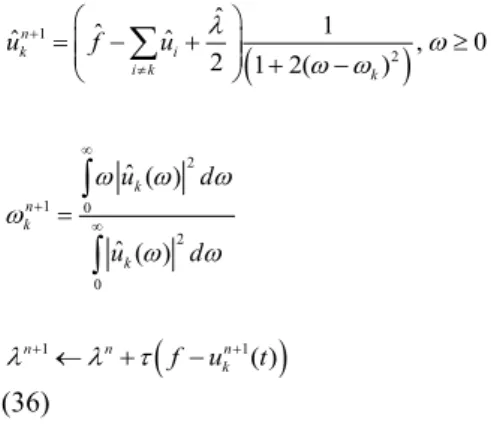
_kat the n+1 the iteration is as follows. The convergence of the algorithm is given in12.

The final updated equations are given by,

2 ₂ 2 2 , , ( ) ( ) jkt , k k t k k k k k k j L u w t u t e f u f u t Z O D G O S ª§§ · · º w «¨¨ ¸ ¸ » © ¹ «© ¹ » ¬ ¼

¦

(5)

1 2 ˆ ₁ ˆ ˆ ˆ , 0 2 1 2( ) n k i i k _k u f u O Z Z Z z § · t ¨ ¸ ¨ _¸ ©

¦

¹ ₍₃₄₎ 2 1 0 2 0 ˆ ( ) ˆ ( ) k n k k u d u d Z Z Z Z Z Z f f

³

(35)

1 1_{( )} n n n k f u t O _mO W (36)

4.Support Vector Machine

Support Vector Machines (SVM) are widely using supervised classification tool in machine learning. Based on the training data { ... }x x1 n , where

n i

xR , together with class labels { ... }y y1 n where yi { 1,1}, SVM can be

trained to create a model14_{. Using this model, it predicts the class of a new testing sample. The idea in SVM is to}

create a hyperplane as shown in Fig. 1 with a maximum margin(separation for adjacent classes ). This helps to reduce the generalization error for classifying a new data point. Fig. 1 shows a two class problem where a linear separation is achieved using a straight line. But in N-dimensional space, a hyperplane can be used for separation of different classes. In cases where data points are clustered so that linear separation is not possible, the data points can be mapped into feature space (higher dimensional space) where a linear separation is possible. This hyperplane which is linear in feature space will be non linear in its corresponding input space 16_.

Fig. 1. Linear separation of data points using SVM.

Consider a two case scenario. Let x1and x2 be the two variables, the objective of SVM is to find a hyperplane of

the form w x1 1w x2 2 J 0 with the bounding planes w x1 1w x2 2 tJ 1 and w x1 1w x2 2 t J 1. Here J is the

bias term which is scalar. During the training stage, SVM finds the appropriate wi s' and J . Ones these parameters

are found, decision boundary is obtained as _{w x}T _J 0_{, where}_w_{is a vector. When new data point comes, the}

decision for the label is found using the function _{f x}( ) _{sign w x}( T _J)

Maximal margin

Bounding plane

Hyperplane Support Vector

(6)

5.Proposed Methodology

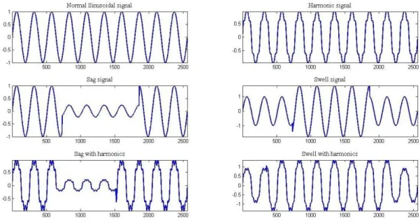
Five different classes of power quality disturbances with their corresponding classes considered are swell-K1, sag-K2, harmonics-K3, sag with harmonics-K4 and swell with harmonics-K5. Also a class K6 with pure sinusoidal signal (50Hz frequency) is included. All signal has 50 Hz normal frequency. Number of samples per cycle is 256 and each signal is ten cycle duration, so every signal consists of 2560 number of total samples. Each class contains 120 cases out of which 100 signals feature vector is used for training the SVM and remaining for testing purpose. Fig. 1 shows one such generated signal from all the six classes considered. Each signal is decomposed in to three IMF candidates. Choosing higher the number of candidates may results in good classification accuracy at the cost of

increase in the dimension of feature vector computational cost. The total size of training matrix is 600 25u . Where

600_{includes 100 cases per class multiplied by 6 classes and 25 includes sines and cosines statistical parameters of}

three IMF candidates together with a label vector. Similarly 120 25u is the dimension of testing data matrix. The

statistical parameters considered are variance, kurtosis, median and range.

Fig. 1. PQ disturbances Waveform.

6.Results and discussion

In the present work, VMD and EWT algorithm is applied for all cases of power signal disturbances which are

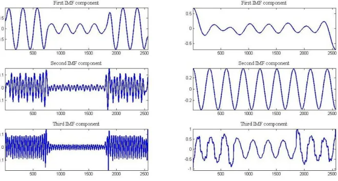
shown in Fig. 1. The estimated three components of sag with harmonic signal is Fig. 2. The D value is set to 2000.

Very low value of D produces high amount of noises in the decomposed modes. It is noticed that the time

complexity of VMD is much higher than EWT. VMD requires around 1918.37 seconds for feature extraction, at the same time EWT requires around 943.14 seconds. The experiments are performed on Windows system having 2.50Ghz Core i5 with 4GB RAM.

(7)

Fig. 2. (a) Three modes extracted using VMD with D 2000; (b) Three modes extracted using EWT.

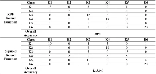
The classification results using SVM for EWT based feature extraction is shown in Table 1. A 6 6u confusion

matrix is created in which diagonal elements shows the correctly classified PQ disturbances and off-diagonal elements represents the misclassified PQ disturbances. The classification accuracy is different for different types of

kernels. An optimum selection of kernel function and parameters gives good classification accuracy16,17,18_{. From the}

confusion matrix obtained, it is noticed that classification results for VMD based feature extraction outperforms the EWT based feature extraction. Table 2 shows the classification results for VMD based feature extraction. Taking more number of statistical parameters with higher number of IMFs may improve the classification accuracy but it will results more time SVM to train.

Table 1. Classification results for EWT using SVM.

SVM Linear Kernel Function Class K1 K2 K3 K4 K5 K6 K1 19 0 1 0 0 0 K2 0 18 1 1 0 0 K3 0 0 20 0 0 0 K4 0 5 4 11 0 0 K5 12 0 2 0 6 0 K6 0 0 0 0 0 20 Overall Accuracy 78.33% Polynomial Kernel Function Class K1 K2 K3 K4 K5 K6 K1 18 0 0 0 2 0 K2 0 20 0 0 0 0 K3 0 0 14 1 5 0 K4 0 1 0 19 0 0 K5 3 0 0 0 17 0 K6 0 0 0 0 0 20 Overall Accuracy 90%

(8)

RBF Kernel Function Class K1 K2 K3 K4 K5 K6 K1 13 0 6 0 1 0 K2 1 14 1 0 4 0 K3 0 0 12 6 2 0 K4 0 1 0 19 0 0 K5 1 0 1 0 18 0 K6 0 0 0 0 0 20 Overall Accuracy 80% Sigmoid Kernel Function Class K1 K2 K3 K4 K5 K6 K1 10 0 4 5 0 1 K2 1 6 3 10 0 0 K3 0 0 5 0 15 0 K4 5 2 1 6 5 1 K5 0 0 11 0 5 4 K6 0 0 0 0 0 20 Overall Accuracy 43.33%

Table 2.Classification results for VMD using SVM

SVM Linear Kernel Function Class K1 K2 K3 K4 K5 K6 K1 17 3 0 0 0 0 K2 0 16 0 4 0 0 K3 0 0 20 0 0 0 K4 0 1 9 10 0 0 K5 0 0 4 0 16 0 K6 0 0 0 0 0 20 Overall Accuracy 82.50% Polynomial Kernel Function Class K1 K2 K3 K4 K5 K6 K1 20 0 0 0 0 0 K2 0 20 0 0 0 0 K3 0 0 20 0 0 0 K4 0 0 0 20 0 0 K5 0 0 0 0 20 0 K6 0 0 0 0 0 20 Overall Accuracy 100% RBF Kernel Function Class K1 K2 K3 K4 K5 K6 K1 19 0 0 1 0 0 K2 0 20 0 0 0 0 K3 0 2 17 1 0 0 K4 0 0 2 17 1 0 K5 1 0 0 0 19 0 K6 0 0 0 0 0 20 Overall Accuracy 93.33% Sigmoid Kernel Function Class K1 K2 K3 K4 K5 K6 K1 13 0 0 1 6 0 K2 5 10 0 5 0 0 K3 0 0 11 6 0 3 K4 0 3 2 14 0 1 K5 4 0 0 0 16 0 K6 0 0 0 0 0 20 Overall Accuracy 70%

(9)

7.Conclusion

This paper considers the classification of power quality disturbances using SVM applied on feature extracted from the signals using EWT and VMD. It is the purpose of this work to introduce recent adaptive signal processing method called VMD which can accurately separate the harmonic components of non-stationary signals regardless of how close their frequency components are. Unlike EWT, without any wavelet filter bank, VMD model is able to generate IMF components concurrently using ADMM optimization method. It can be concluded that the

effectiveness of VMD can replace ordinary method like EMD which doesn’t have a strong mathematical foundation

and EWT which builds adaptive wavelets for signal decomposition. Instead of directly taking the statistical parameters of different modes as feature vector, it is found that the feature vector derived by taking sines and cosines of statistical parameters of modes gives better classification accuracy and less time SVM to converge during training. A good automated system for maintaining the power quality requires detection, identification and classification of power quality disturbances.

References

1. S. Taskin, H. Gokozan. Determination of the spectral properties and harmonic levels for driving an induction motor by an inverter driver under the different load conditions. Elektronika ir Elektrotechnika(Electronics and Electrical Engineering). no. 2. p.75–80. 2011.

2. J. Chung, E. J. Powers, W. M. Grady, and S. C. Bhatt. Power disturbance classifier using a rule-based method and wavelet packet-based hidden markov model. IEEE Trans. Power Delivery. vol. 17. p.233–241. Jan. 2002.

3. A. K. Ghosh and D. L. Lubkeman. The classification of power system disturbance waveforms using a neural network approach. IEEE Trans. Power Delivery. vol. 10. p. 109–115. Jan. 1995.

4. G. Rata, M. Rata, C. Filote, Theoretical and experimental aspects concerning Fourier and wavelet analysis for deforming consumers in power network. ElektronikairElektrotechnika (Electronics and Electrical Engineering). no. 1. p. 62–66, 2010.

5. S. Chen, H. Y. Zhu. Wavelet Transform for Processing Power Quality Disturbances. EURASIP Journal on Advances in SignalProcessing. 2007.

6. S. Santoso, J. Lamoree, W. M. Grady, E. J. Powers, and S. C. Bhatt. A scalable PQ event identification system. IEEE Trans. Power Delivery. vol. 15. p.738–743. Apr 2000.

7.Jerome Gilles. Empirical wavelet transform. IEEE transactions on signal processing. vol. 61, no.16.August 15, 2013.

8. N.E. Huang, Z. Shen, S.R. Long, M.L. Wu, H.H. Shih, Q. Zheng, N.C. Yen, C.C. Tung and H.H. Liu. The empirical mode decomposition and Hilbert spectrum for nonlinear and non-stationary time series analysis. Proc. Roy. Soc. LondonSeriesA:Mathematical, Physical and Engineering Sciences. vol. 454, no.1971. p.903–995. 1998.

9. M. E. Torres, M. A. Colominas, G. Schlotthauer, and P. Flandrin. A complete ensemble empirical mode decomposition with adaptive noise. Proc. IEEE Int. Conf. Acoust., Speech Signal Process.(ICASSP). p. 4144–4147. May 2011.

10. S. Liu, Q. He, R. X. Gao, and P. Freedson. Empirical mode decomposition applied to tissue artifact removal from respiratory signal. IEEE Engineering in Medicine and Biology Conference (EMBC). p.3624– 3627. Jan. 2008.

11. I. Mostafanezhad, O. Boric-Lubecke, V. Lubecke, and D. P. Mandic. Application of empirical mode decomposition in removing fidgeting interference in doppler radar life signs monitoring devices. IEEE Engineering in Medicine and Biology Conference (EMBC). p.340– 343. Jan. 2009.

12.Konstantin Dragomiretskiy and Dominique Zosso. Variational Mode Decomposition. IEEE Transactions on Signal Processing. vol. 62, no. 3. p.531–544. Feb.2014.

13.Stephen Boyd, Neal Parikh, Eric Chu, Borja Peleato and Jonathan Eckstein. Distributed Optimization and Statistical Learning via the Alternating Direction Method of Multipliers. Foundations and Trends in Machine Learning. vol. 3, no.1. p.1–122. 2010.

14. Dr. K. P. Soman, Ajav. V, Loganathan R. Machine Learning with SVM and other Kernel Methods. PHI Learning Pvt. Ltd. 2009. 15. Thorsten Joachims. Transductive Inference for Text Classification using Support Vector Machines. In Proceedings of the Sixteenth International Conference on Machine Learning (ICML '99), Ivan Bratko and SasoDzeroski (Eds.). Morgan Kaufmann Publishers Inc, San Francisco, CA,USA,p.200-209. 1999.

16. B. Scholkopf, A. Smola, R. C.Williamson, and P. L. Bartlett. New support vector algorithms. Neural Computation. vol. 12. p.1207-1245. May 2000.

17. V. Vapnik. Statistical Learning Theory. Wiley. 1998.