Yang Liu
Helsinki February 12, 2020
Master’s thesis
UNIVERSITY OF HELSINKI
Faculty of Science Computer Science Yang Liu
Assessing text readability and quality with language models
Dorota Glowacka and Alan Medlar
Master’s thesis February 12, 2020 57 pages + 0 appendices
Text readability, text quality, language models, LSTM, GPT-2, case study
Automatic readability assessment is considered as a challenging task in NLP due to its high degree of subjectivity. The majority prior work in assessing readability has focused on identifying the level of education necessary for comprehension without the consideration of text quality, i.e., how naturally the text flows from the perspective of a native speaker. Therefore, in this thesis, we aim to use language models, trained on well-written prose, to measure not only text readability in terms of comprehension but text quality.
In this thesis, we developed two word-level metrics based on the concordance of article text with predictions made using language models to assess text readability and quality. We evaluate both metrics on a set of corpora used for readability assessment or automated essay scoring (AES) by measuring the correlation between scores assigned by our metrics and human raters. According to the experimental results, our metrics are strongly correlated with text quality, which achieve 0.4-0.6 correlations on 7 out of 9 datasets. We demonstrate that GPT-2 surpasses other language models, including the bigram model, LSTM, and bidirectional LSTM, on the task of estimating text quality in a zero-shot setting, and GPT-2 perplexity-based measure is a reasonable indicator for text quality evaluation.
ACM Computing Classification System (CCS):
Computing methodologies→Artificial intelligence →Natural language processing Applied computing→Document management and text processing
Tekijä — Författare — Author Työn nimi — Arbetets titel — Title Ohjaajat — Handledare — Supervisors
Työn laji — Arbetets art — Level Aika — Datum — Month and year Sivumäärä — Sidoantal — Number of pages Tiivistelmä — Referat — Abstract
Avainsanat — Nyckelord — Keywords
Säilytyspaikka — Förvaringsställe — Where deposited Muita tietoja — övriga uppgifter — Additional information
Contents
1 Introduction 1
2 Related work 2
2.1 Text readability assessment . . . 3
2.1.1 Traditional readability measures . . . 3
2.1.2 Cognitive and discourse features . . . 5
2.1.3 Language models . . . 5
2.2 Text quality assessment . . . 6
2.2.1 Shallow NLP techniques . . . 7
2.2.2 Full NLP techniques . . . 8
2.2.3 Deep learning techniques . . . 9
3 Language models 10 3.1 Language model basics . . . 11
3.1.1 Introduction . . . 11
3.1.2 Evaluation of language models . . . 12
3.2 Statistical language models . . . 13
3.3 Neural network based language models . . . 16
3.3.1 Neural networks . . . 17
3.3.2 Neural network language model . . . 20
3.3.3 Recurrent neural network based language model . . . 21
3.3.4 Attention mechanism and the Transformer . . . 24
3.3.5 Pre-trained language models . . . 26
4 Methodology 29 4.1 Dataset description . . . 30
4.1.1 The Guardian Corpus . . . 30
4.1.3 The OneStopEnglish Corpus . . . 31
4.1.4 The WeeBit Corpus: . . . 31
4.1.5 The IELTS Corpus . . . 32
4.1.6 The ASAP Dataset . . . 32
4.2 Model description . . . 33
4.2.1 Bigram language model . . . 34
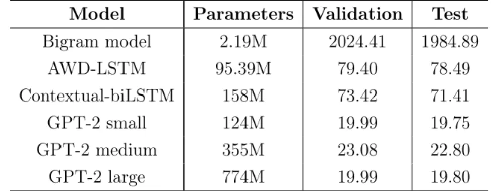
4.2.2 AWD-LSTM . . . 34 4.2.3 Contextual bidirectional LSTM . . . 35 4.2.4 GPT-2 . . . 35 4.2.5 Training results . . . 35 4.3 Word-level metrics . . . 36 4.3.1 Word perplexity . . . 37 4.3.2 Likelihood ratio . . . 37 4.4 Correlation coefficients . . . 38
4.4.1 Pearson correlation coefficient . . . 38
4.4.2 Spearman’s rank correlation coefficient . . . 39
5 Experiments 39 5.1 Correlation experiments on text readability . . . 39
5.1.1 Experimental setup . . . 40
5.1.2 Results . . . 40
5.2 Correlation experiments on text quality . . . 42
5.2.1 Experimental setup . . . 43
5.2.2 Results . . . 43
5.3 Discussion . . . 46
5.3.1 Word perplexity VS likelihood ratio . . . 46
5.3.2 A case study of text quality evaluation . . . 47
1
Introduction
Readability describes the complex relationship between a given text and the effort that readers make to understand it. Nowadays, people are increasingly relying on online materials to acquire knowledge. This greatly raises readers’ expectations for the readability of materials. Take the largest Online Encyclopedia - Wikipedia as an example, although Wikipedia has been shown to be highly accurate in terms of factual content, it has been criticized for the quality of its writing, with many arti-cles suffering from poor readability and style [1]. However, given the size of online texts, identifying article readability to enable not only the selection of appropri-ate mappropri-aterials for readers but editing suggestions for editors requires an automappropri-ated approach.
A majority of the prior work in assessing readability has focused on identifying the level of education necessary for comprehension, which is generally expressed as the American grade level (i.e. years of primary and secondary education) [2, 3, 4, 5]. But the problem we want to explore here does not only assess readability in terms of comprehension, but in terms of style. Namely, do articles contain well-written, idiomatic prose that reads naturally to a native speaker of English. This is somehow similar to another task in literature called automated essay scoring (AES) that evaluates either contextual accuracy or writing quality of articles by automatically assigning goodness scores based on multiple criteria, such as word choices, narrativity, organization, and so on [6]. In this thesis, we studied these two aspects of readability, i.e., comprehension and style, which are referred to as readability assessment and text quality evaluation separately.
In this thesis, we propose two readability metrics: average per word perplexity and average likelihood ratio, based on the concordance of article text with predictions made using neural language models. Our goal is not to develop a classifier for "good" or "bad" writing, but to design metrics that allow us to rank documents, paragraphs and sentences by the degree to which text conforms to a corpus of documents that are assumed a priori to be highly readable and well-written. As both metrics are based on language models, they are unsupervised and do not require any special annotation.
In our experiments, the language model was trained using articles from The Guardian, a British newspaper, that we believe are well-written because they are written by professional journalists. Both metrics serve a dual purpose as they can be used to
(i) rank documents from the least to most readable, allowing us to identify which articles are most in need of attention in terms of writing quality and style and, (ii) use highlighting on a per word basis in the article to help an editor identify whether there are specific issues that should be fixed or that the entire article needs to be rewritten.
In this work, we make the following contributions:
1. We take an unsupervised ranking-based approach that identifies how well ar-ticles fit a model trained on well-written text. While existing approaches to assess the writing readability and quality are mostly based on supervised learning methods.
2. We demonstrate that our metrics are strongly correlated with text quality, i.e., whether an article is idiomatic and well-written, and have a weak correlation with text readability in terms of comprehension.
3. We explored the suitability of different types of language models, including a bigram model, LSTM, bidirectional LSTM, and GPT-2. We demonstrate that GPT-2 achieves the performance far beyond other language models on text quality assessment in a zero-shot setting.
This thesis consists of six chapters. Chapter 2 introduces the related works of both tasks i.e. readability assessment and text quality evaluation. In Chapter 3, we focus on the basis of language models and describes several widely used architectures in language modeling. Chapter 4 dives into the method we use for the task of text readability and quality evaluation. The description of datasets and language models used for performing experiments are also included here. In Chapter 5, we describe the experimental setup and analyze the results obtained. Chapter 6 contains the conclusion and suggestions for future work.
2
Related work
As we discuss the measurements of both text readability and quality in this thesis, it is necessary to introduce the related works and backgrounds in both fields. There-fore, section 2.1 will describe the related works of text readability assessment while we dedicated section 2.2 to the previous approaches to automated essay scoring.
2.1
Text readability assessment
Readability describes a complex relation between a given text and the efforts that readers make to understand it. The relation is considered to be associated with multiple factors, including lexical simplicity, presentation style, discourse cohesion, and background information [7]. Historically, interest in readability assessment in terms of comprehension originated in education and the military [8, 9]. Nowadays, in most cases, the research on readability assessment often identifies the level of education necessary for comprehension [2, 10]. Due to the high degree of cognitive complexity, readability assessment is considered as one of the most challenging tasks and therefore has attracted researchers’ attention to explore automatic approaches for it [2, 3, 10, 11].
A variety of approaches were investigated to find readability measures that corre-late well with human perception over the past few decades. Traditional readability measures were formulated by straightforward discrete features such as average sen-tence length, word length and difficulty and so on. Among them, Dale-Chall [12], Gunning’s Fog (FOG, [8]), Flesch-Kincaid [9], and SMOG (Simple Measure of Gob-bledygook, [13]) indexes, as the most representative traditional formulas, will be introduced in section 2.1.1. Instead of shallow features, some cognitively motivated features and discourse features were adopted to classify the readability level of texts, which will be described in section 2.1.2. As we mainly used language models to mea-sure the readability in this thesis, we dedicated section 2.1.3 to the use of different language models on readability evaluation.
2.1.1 Traditional readability measures
Traditional readability formulas use shallow linguistic features, including the number of words, sentences and syllables, to output a readability score.
The first widely adopted readability measure, Dale-Chall readability formula (DCRF, [12]), was proposed in 1948. DCRF utilizes a manually curated list of easy to un-derstand words, with all others deemed to be "difficult" words, to measure the text readability. It is calculated according to Equation 1:
DCRF = 0.1579(C(Difficult words)
C(T otal words) ×100) + 0.0496
C(T otal words)
C(T otal sentences), (1)
whereC is a counting function. If the percentage of difficult words is above 5%, we should add 3.6365 to the raw score to obtain the adjusted score. When assessing
texts, a higher Dale-Chall score indicates that the text is more difficult to read.
Subsequently, in 1952, Gunning [8] proposed the Gunning fog index (GFI), in order to estimate the grade level required to understand text on the first reading. It was formulated as follows:
GF I = 0.4×[ C(T otal words)
C(T otal sentences) + 100
C(Complex words)
C(T otal words) ], (2)
where Complex words refers to words that consists of three or more syllables. In-tuitively, the higher the GFI index, the less readable the text.
In 1975, Flesch-Kincaid readability tests were used to assess the readability of tech-nical manuals in the United States military [9]. There were two tests: the Flesch Reading Ease Score (FRES) and the Flesch-Kincaid Grade Level (FKGL). Both tests utilized the total number of syllables, words and sentences to approximate the reading ease score and corresponding grade level of a text. However, they employed different weighting factors obtained by performing regression on a dataset of Naval school passages [9]. Their formulas are listed below,
F RES = 206.835−1.015 C(T otal words)
C(T otal sentences) −84.6 C(T otal syllables) C(T otal words) , F KGL= 0.39 C(T otal words) C(T otal sentences)+ 11.8 C(T otal syllables) C(T otal words) −15.59. (3)
In the Flesch Reading Ease test, the higher FRES implies that the text is easier to read. While in the Flesch–Kincaid Grade Level test, FKGL directly corresponds to a U.S. grade level.
Similar to FKGL formula, SMOG (Simple Measure of Gobbledygook, [13]), is used to estimate the years of education needed to comprehend the given texts adopting the number of polysyllables and sentences as features. SMOG is calculated according to the following formula:
SM OG = 1.0430
s
C(P olysyllables)× 30
C(T otal sentences) + 3.1291, (4)
where C(P olysyllables) means the number of words that contain more than three syllables. In practice, SMOG is only applicable if the text has more than 30 sentences as it was normed on 30-sentence samples.
All readability assessment formulas cited above operate at the level of document, whether that is a technical manual, book or web page. Based on the above formulas, the use of shallow features will return the same score if we shuffled the order of
words in each sentence. This suggests that traditional readability measures are easily cheated. In addition, the parameters of these formulas were obtained using some specific dataset and might not be transferable to other datasets [14].
2.1.2 Cognitive and discourse features
To overcome the deficiencies of traditional readability measures, multiple approaches that used complex syntactic and semantic features to predict the readability level have been proposed. These approaches usually require extensive feature engineering and, therefore, can achieve much better results in readability assessment.
Feng et al.(2009, [3]) produced an automatic readability metric that is tailored to the literacy skills of adults with intellectual disabilities (ID). They investigated multiple discourse-level, cognitively motivated features that correlate with the readability level for adults with ID, such as total number of nouns and name entities, number of unique entities, and the average lexical chain span. They argued that the use of audience-specific features can improve the accuracy of readability assessment on the specific user group.
Recently, Mesgar and Strube (2018, [11]) proposed a local coherence model that identifies whether adjacent sentences are semantically similar. They adopt a recur-rent neural network (RNN) to represent semantic information that connects two adjacent sentences and then employed a convolutional neural network (CNN) to en-code the pattern of semantic information changes across sentences. As a result, the model achieves new state-of-the-art results on the task of readability assessment.
Although the use of cognitive and discourse features improves the accuracy of read-ability assessment, it has been criticized for the requirement of sophisticated manual feature engineering [15].
2.1.3 Language models
It is well noted that language models can capture linguistic features well and, there-fore, have been widely used to evaluate text readability.
Initially, researchers in computational linguistics have adopted statistical language models that extract context information from texts to improve the accuracy of read-ability assessment. In 2001, Si and Callan [2] classified scientific web pages of dif-ferent grade levels based on a unigram language model. They built a reading level
classifier by linearly combined a unigram model and surface linguistic features. It was shown that their method surpasses the widely used Flesch-Kincaid readability formula.
In the work of Schwarm and Ostendorf (2005 and 2009, [10, 16]), SVM-based de-tectors that incorporate the perplexity from unigram, bigram and trigram language models and other traditional features were created to perform readability assess-ment. They investigated the influence of syntactic features and traditional lexical features on estimating accuracy and explored the alternative regression model to the SVM classifier in the context of limited annotated training data.
Later on, the introduction of neural language models has achieved better results for the task of readability assessment. Azpiazu and Pera (2019, [15]) proposed a multi-attentive long-short term memory (LSTM) architecture called Vec2Read for automatic multilingual readability assessment. The model leveraged a multi-attentive strategy to make the network concentrate on specific words, sentences, and paragraphs that correlated with reading levels and then predicts probability over reading levels based on attention scores. The use of attention mechanism yields better results than the same LSTM architecture with traditional and deep learning strategies.
Martinc et al. (2019, [7]) presented both supervised and unsupervised approaches with multiple novel neural language models, such as LSTM and BERT (Bidirec-tional Encoder Representations from Transformers, [17]), on readability estimation. It was shown that the supervised approach they employed achieved better results than traditional readability formulas and is transferable across languages. It is worth mentioning that they directly used model perplexity as a metric for assessing readability on an unsupervised setting, which coincided with our idea. However, their perplexity-based measures were concluded as the worst measurements accord-ing to their experimental results. In this thesis, we argue that perplexity is a strong indicator of text quality evaluation.
2.2
Text quality assessment
Text quality assessment is a task to evaluate how well-written an essay or article is by assigning a goodness score to it, which is often referred to as AES. AES aimed to relieve the heavy work loads of educators or teachers in assessing large amounts of essays and can be traced back to the 1960s when the first AES system Project Essay Grade (PEG) was proposed [18]. Since then, researchers have considered AES as a
regression, classification and preference ranking problem and utilized uncountable statistics, machine learning and deep learning techniques to approach it [19, 20].
We can classify existing approaches for AES according to the level of NLP (short for Natural language processing) techniques applied [6]. Based on this, three cate-gories could be identified: shallow NLP refers to statistical techniques for shallow linguistic features, i.e. lexical level features, full NLP involves more sophisticated NLP techniques for not only lexical level but syntax, semantics and structure level features, deep learning NLP involves advanced deep learning architectures, such as RNN, CNN and neural attention models for automatic feature selection [6, 20, 21].
Therefore, in this section, we will follow these three categories to briefly introduce the development of AES systems and approaches.
2.2.1 Shallow NLP techniques
The early AES systems mainly used statistical analysis of one or multiple shallow linguistic features, i.e. lexical level features, such as keyword frequency or punctu-ation counts. The PGE proposed by Page et al.(1966, [18]), the Intelligent Essay Assessor (IEA) introduced by Thomas et al.(1997, [22]) and E-rater presented by Burstein et al.(1998, [23]) are three of the most representative AES systems in this category.
PEG predicted essay scores using regression with up to 30 parameters, such as average word length, number of semicolons, and word rarity [18, 24]. As the first AES system, despite critics arguing that computers cannot determine the writing competence as well as humans does, it proved that the PEG score correlated well with scores by human raters. However, PEG can only capture writing style rather than contents of essays as only shallow linguistic features were used. Despite this, PEG has been widely used due to its conceptual simplicity and limited computer requirements[21, 25, 26].
IEA used latent semantic analysis (LSA, [22]) to grade essays automatically, which was first designed for information retrieval to measure the similarity between docu-ments. The underlying principle of LSA is to identify the semantic similarity between the input document and indexing documents by converting documents into vectors based on the frequency of indexed terms in the input document. Then, the IEA system will assign a goodness score using the average score of several most similar calibration documents. The number of calibration documents used is predefined as
a hyper-parameter. Contrary to PEG, IEA can capture contents of essays instead of writing style due to the nature of the LSA method. It is also reported a high correlation between IEA scored and human scored essays [26].
Compared to PEG and IEA, E-rater has more sophisticated architecture which contains three modules corresponding to syntactic variety, discourse structure, and content analysis. Syntactic variety was represented using the ratio of complement, subordinate, infinitive, and relative clause and occurrences of modal verbs per sen-tence per essay. Discourse structure was similar to PEG but with up to 60 variables. Content analysis aimed to measure the semantic similarity between essays, which shares the same concept as the IEA system. It was shown that E-rater correlates significantly with human raters [23]. E-rater is the superior choice for grading con-tent and has been used to score the General Management Aptitude Test (GMAT) [23, 26].
Other existing approaches, such as Larkey’s system (1998, [27]), formulated AES as a classification task and applied the classical Naive Bayes model. Further, multino-mial Bernoulli Naive Bayes was used to classify the categories of text quality[28]. Despite the fact that shallow features can hardly capture the semantic information, it is consistently reported that multiple systems or approaches using shallow NLP techniques could achieve 60% exact agreements with human raters [21, 6, 26].
2.2.2 Full NLP techniques
Due to the limitation of shallow features, early systems could not capture the dis-course cohesion and semantic information when evaluating the text quality. As a result, they are more likely to be tricked by some nonsense essays generated inten-tionally. For example, IEA could be fooled to give a high score to a text that consists of a sequence of relevant words without any structure [26].
Therefore, to eliminate the limitation, more complicated NLP tools were applied into AES systems and approaches, including syntactic analyzers, rhetorical parsers, and semantic analyzers. Rhetorical parsers aimed to determine the discourse structure of texts [29]. Syntactic analyzers were used to identify sentence components and analyze syntactic dependencies between them [30]. While semantic analyzers were utilized to identify the function of each component in the text [6, 31].
C-rater (2001, [23]) and its advanced version E-rater (2006, [32]) are two most popular systems that were benefited from these NLP tools. C-rater and E-rater
are automated scoring systems that were designed for Educational Testing Service (ETS), the largest nonprofit educational testing and assessment organization in En-glish. Both of them made use of not only the lexical level features but more complex syntactic features extracted from the training texts. As a result, they achieved high percentage agreements (over 80% agreement) with human raters in both small-scale and large-scale studies [6].
Subsequently, a new series of ranking-based methods were proposed, combined with complex NLP tools. In 2011, Yannakoudakis et al. formulated the AES task as a preference ranking problem [33]. It made use of hybrid features containing word n-grams, part-of-speech n-grams, grammatical complexity, and parsing trees to rank the order of essays based on the writing quality and then measured the correlation between system scores and human graders’ scores. Further, Chen et al. [34] applied a list-wise ranking technique into their system in order to reduce biases between human raters and computer based systems by directly incorporated the agreements term into the loss function. The features they utilized included syntactic variety, sentence fluency, and prompt-specific features.
2.2.3 Deep learning techniques
Despite the fact that full NLP techniques based systems achieved fantastic per-formance on AES, they required sophisticated manual feature engineering [6]. To combat this issue, people began to explore more advanced approaches that made use of state-of-the-art deep learning techniques to learn syntactic and semantic features automatically.
It should be mentioned that there was no existing benchmarks that could be used to uniformly evaluate AES systems until Shermis and Burstein presented the Auto-mated Student Assessment Prize (ASAP) dataset in 2013 [19]. Subsequently, with the emergence of powerful deep learning tools and the benchmark dataset, significant progress have been made on the AES task.
In 2016, Alikaniotis et al. adopted a LSTM based language model to perform AES. The model took the word embeddings that were learned by the word contributions to text score as input, and obtained the essay expression using the last hidden states of a two-layer bidirectional LSTM. The LSTM based model achieved excellent re-sults, outperforming other commonly used systems [35]. Further, Taghipour and Ng [36] explored several neural network models including LSTM, LSTM with attention
mechanism, CNN combined with LSTM and bidirectional LSTM for the AES task. Their method avoided a large amount of effort to perform feature engineering and the best architecture, LSTM, outperformed a strong baseline by 5.6% in terms of the Kappa coefficient.
Subsequently, CNN were also adopt for AES. Dong and Zhang (2016, [37]) employed a hierarchical CNN on the AES task. It split texts into sentences and extracted both sentence-level and text-level information using a two-layer CNN to obtain the text representation. This method was demonstrated to outperform the baseline approaches, such as Bayesian Linear Ridge Regression (BLRR) and Support Vec-tor Regression (SVR), showing automatically learned features to be competitive to handcrafted features. Dong et al.(2017, [20]) systematically investigated CNN and LSTM on sentence-level and text-level representation respectively, and the effective-ness of attention mechanism on automatically selecting more relevant n-grams and sentences for the task. It was proved that the method outperforms the previous methods and attention mechanism is particularly effective in the AES tasks.
Our work combines neural networks with an unsupervised ranking-based method to provide further help for writing and editing. Results shows that our metrics strongly correlate with quality scores graded by human raters.
3
Language models
Language modeling is an approach to understanding linguistic structures within the language by learning from corpus data. The studies of language structures can be traced back to two centuries ago [38]. Since then, linguists have accumulated a large number of corpora to find syntactic rules of the language. These rules were formalized into the grammar that we know today [39]. While grammar can indeed recapitulate the structure and usage of the language, they cannot completely identify all situations that occur in language use as people may sometimes speak ungrammatically to meet their daily communication needs [40]. Therefore, in order to address this problem, scientists have instead made use of statistics as a tool to identify the common patterns within languages. More specifically, language models could learn the probability distribution of words that occurred in a sequence from corpus data. This kind of approach is called language modeling [41].
Language models are probabilistic models that assign probabilities to words or se-quences. More specifically, given a corpus C, language models can learn the
condi-tional probability distribution p(w|c), the probability of a word w appearing in the contextc. According to this, language models can be used to predict the probability with each possible next word occurred and generate text by continuously sampling from the probability distribution [38].
There are two main categories of language models: statistical language models (SLM) and neural network based language models (NNLM). SLM was first proposed in 1980, and then widely used in a variety of NLP tasks that rely on probability of words or sequences [42]. For example, statistical language models were used to assign a goodness score based on the probability that a sequence occurred and therefore could suggest the most accurate translation for machine translation tasks or the most likely transcription in speech recognition [43, 44, 45, 46]. However nowa-days, powerful neural networks based language models have replaced the statistical models and become dominant in NLP. These neural language models have achieved state-of-the-art performance on a large amount of challenging NLP tasks like ma-chine translation, speech recognition, and natural language inference [47, 48, 49, 50]. Here, we aim to introduce our new word-level metrics to assess the text readability and quality. As the metrics we proposed are actually mathematical variants of the word probability that language models output, it is greatly necessary to introduce the theoretical background of language models before we delve into the details of the metrics. In this chapter, the details of language model basics and the formulas as well as architectures of multiple language models will be described.
3.1
Language model basics
In this section, we will introduce the flow of building a language model and its evaluation, in order to help readers understand model details better. Section 2.1 describes language representation and the training process, while section 2.2 depicts evaluation methods of language models in detail.
3.1.1 Introduction
Building a language model often requires three compulsory steps, which are process-ing the corpus, trainprocess-ing the language model, as well as fine-tunprocess-ing and evaluatprocess-ing the trained model. Assuming that we have a clean corpus that is ready for training and we want to build a language model based on it, the first thing to do will be splitting the text into tokens and build a vocabulary which is a list of all unique
tokens in the corpus. This step is calledtokenization.
Then, before feeding data into a language model, it is essential to encode tokens into a readable format for a language model. However, different models require different inputs. For statistical language models, encoding is not necessary. As for neural language models which require the input sequence to be a vector or matrix, there are two commonly used ways to encode tokens, which are calledone-hot encoding and word embedding.
One-hot encoding is a method to convert each token into a unique one-hot vector. One-hot vector consists of all 0s, except for a single 1 in some position. For a vocabulary of sizeN, the n-th one-hot vector is the vector whose n-th entry is 1 and all other entries are 0s. Therefore, there would be a total of N one-hot vectors that could represent allN unique tokens. These one-hot vectors could be either directly fed into models or stacked as batches. One-hot encoding is easy to make and highly interpretable for language model use. However, it leads to a higher level of sparsity as the vocabulary size increases [41].
Another popular approach for encoding is word embedding, which was first intro-duced in the 1960s [51]. Word embedding represents a set of techniques where distributed representations of individual tokens are learned based on the usage of tokens [52]. It is used to map unique tokens into vectors with a fixed length. These vectors obtained by statistical or machine learning methods are supposed to capture the semantic similarities between linguistic items. Word embedding does not only address the sparsity issue of one-hot encoding but also provides semantic information for language models. Therefore, a large amount of language models and downstream NLP tasks take word embedding as the very first step to conduct [52, 53].
3.1.2 Evaluation of language models
Intuitively, we can evaluate the performance of a language model by measuring the improvements that the model made on a specific NLP task. For example, in speech recognition, we can compare the output of the speech recognizer with different language models to see which language model leads to a more concise transcription. This kind of end-to-end evaluation is called extrinsic evaluation [41]. Extrinsic evaluation is considered to be the best way to evaluate language models because they can better serve the tasks we are performing [41].
expensive as those downstream NLP applications often have more complex architec-tures [41]. Therefore, it is essential to instead create intrinsic evaluation metrics that are independent of any application and directly measure the performance of a language model. The most commonly used metric is called perplexity.
It is commonly used to evaluate a language model by computing the average per-plexity on the test set. The perper-plexity describes the degree of uncertainty that the model feels about the sequence of interest. It is defined as the normalized inverse of the probability of that sequence under the language model. For a sequence of words
W =w1w2...wN that of size N, the perplexity (PP for short) is formulated as [41]:
P P(W) = N
s
1
p(w1w2...wN)
. (5)
According to Equation 5, we can conclude that the higher the probability of a sequence, the lower the perplexity. Basically, we expect that the language model is confident of sequences that appeared in the corpus on which the model was trained. That is to say, the probabilities of sequences in the corpus should be high and the perplexity of those sequences should be low.
3.2
Statistical language models
Statistical language models directly model the conditional probability distribution of a word given the words that precede it. That is to say, given a sequence of words
w1w2...wm, SLMs will compute the probability of p(wn|w1w2...wm−1) by calculating
the ratio of the number of times that the history sequence sold = w1w2...wm−1
followed by wordwm to the number of times that sold occurs in the given corpus, as shown in Equation 6 [41].
p(wm|w1w2...wm−1) =
C(w1w2...wm−1wm)
C(w1w2...wm−1)
, (6)
where the capitalC stands for a counting function.
SLMs can also be used to compute the joint probability of an entire sequence ac-cording to the chain rule of probability [41]:
p(w1w2...wm) =p(w1)p(w2|w1)p(w3|w1w2)...p(wm|w1w2...wm−1). (7)
With the ability to assign probabilities to words or sentences, SLMs are widely used in speech or optical character recognition, spelling or grammatical error correction as well as machine translation tasks [39, 41].
It is intuitive that the relation between the very beginning wordw1 and the last word
wm will be extremely weak as the length of the sequence increases. Therefore, we assume that, for a wordwm, its probability of appearing in the end of the sequence
w1w2...wm−1 only depends onnprevious words rather than all previous words. Based
on it, Equation 6 and 7 will be converted into:
p(wm|w1w2...wm−1)≈p(wm|wm−n...wm−1), (8)
p(w1w2...wm) =p(wm−n)p(wm−n+1|wm−n)...p(wm|w1w2...wm−n). (9)
This kind of models are considered to have a sliding window of size n and are calledn-gram language models. Here, the n-gram is responsible for a sequence of size n. Similarly, the bigram (or 2-gram) represents a two-word sequence and trigram(also called 3-gram) stands for a sequence of three words or tokens [41]. As the size of the sliding window n increases, the complexity of the model and the model size increases as well. For a corpus that has N unique tokens, if we want to model the conditional probability that a sequence of size n −1 followed by a wordwn, we have to count how many times that Nnn-grams andNn−1 (n-1)-grams appear in the corpus according to Equation 8 and 9. As a result, the model size will be extremely large when n is a large number. Therefore, n is often smaller than 5 in practice.
Whenn = 1 (the uni-gram model), it is suggested that the probability of each word only depends on its own probability in the given corpus. The Equation 9 is simplified asp(w1w2...wm) = p(w1)p(w2)...p(wm). Despite the fact that the uni-gram model is easy to use, it cannot capture contextual information compared to higher dimension language models. The bi-gram model computes the conditional probability of a sequence w1w2...wm−1 followed by a word wm by the conditional probability of a wordwn appearing after its previous word wn−1. Note that the bi-gram model is a
variant of theMarkov model, which is a kind of classical probabilistic model used for modeling randomly changing systems [41].
Despite the fact that model complexity increases as window size n and vocabulary size N increase, it is understandable that higher-order n-gram models will do a better job on language modeling on corpora that have suitable sizes. However, other than the large increase of model complexity, higher-order n-gram models have another problem called thecurse of dimensionality [41, 39]. This term describes the phenomenon that sparsity of the corpus increases as the model dimensionality increases. Specially, it is difficult to accurately estimate the probability of n-grams
that rarely or never appeared in the corpus, because those n-grams may be just missing from the corpus as any corpus is limited. Therefore, it is not reasonable to assign them an extremely low or even zero probabilities with the consideration of generalization.
The method used to solve the sparsity problem in SLMs is calledsmoothing, which gets rid of the extremely low or zero probabilities by adjusting the maximum like-lihood estimator of language models [41]. Smoothing is utilized to deal with the problem that n-grams did not appear in the training corpus but are in the unseen test dataset. Before that, how do we address words from the test corpus that are not in the vocabulary? Normally, we replace those words with an unkown marker such as <UNK> and then treat <UNK> as a normal word. After that, we use smoothing to solve those n-grams that the model did not see in the training corpus.
The most used smoothing methods are Laplace smoothing, add-k smoothing, stupid backoff and Kneser-Ney smoothing. Laplace smoothing (also called add-1 smoothing) is to add 1 to all counts of n-grams. Using bi-gram model as an example, the conditional probability is modified as follows, where N represents for the number of bi-grams in the corpus [41].
p(wn|wn−1) = C(wn−1wn) C(wn−1) , (10) p(wn|wn−1) = C(wn−1wn) + 1 C(wn−1) +N . (11)
In this way, all zero probabilities are convert to a small number N+1V, assuming that the vocabulary has sizeV. This is of benefit for estimating the probabilities of sequences in test dataset. However, it is suggested that Laplace smoothing is not a good choice for language models, because it will assign the same probabilities to each unseen token. Despite this, it is considered as a baseline for other smoothing methods in SLMs [41].
Add-k smoothing shares the same concept with Laplace smoothing. It instead adds
k to counts for n-grams as shown in the following [41]:
p(wn|wn−1) =
C(wn−1wn) +k
C(wn−1) +k∗N
. (12)
It is often beneficial to fine-tune k by optimizing it on a validation set. Therefore, add-k smoothing is considered a more flexible approach than add-1 smoothing. How-ever, add-k smoothing suffers from the same deficiency of generating probabilities with poor variance as the add-1 smoothing does [41, 54].
The stupid backoff smoothing is quite a different approach compared to add-1 and add-k smoothing, which substitute the probability of an n-gram with the proba-bility of its corresponding (n-1)-gram if the n-gram rarely appears in the corpus. Taking trigram model as an example, assuming that we want to compute the condi-tional probability p(wn|wn−1wn−2) but the sequence wn−2wn−1wn are missing from the corpus. What stupid backoff does is estimate the probability using the bigram probability p(wn|wn−1). This step is called backoff. Variants of stupid backoff, such as Katz backoff and Good-Truing backoff generally perform well in prac-tice but fail under some conditions. For example, if the sequencewn−2wn−1wnrarely appears in a corpus, it is possible that the sequence is grammatically incorrect. How-ever, the backoff-based approaches may consider that the corpus is too limited and therefore cause an unsatisfactory result [39, 41].
The most widely used method for smoothing is called Kneser-Ney smoothing. The basic idea behind this method is to discount the probability mass of n-grams by subtracting some discounted ratesdm, where dm is the difference of n-grams counts in training and test sets. That is to say, if all n-grams that occurmtimes in training set and appearm0 times on average in the test set,dm will be computed by m−m0. Other than the discounting issue, the Kneser-Ney method also solves the problem that some unigrams have high probability only because their corresponding n-grams have large counts. It assumes that the continuation probability pcon(wi) of a word
wi is proportional to the number of n-grams thatwi has appeared in. Final formulas of Kneser-Ney smoothing for the bigram model are as follows [41]:
pkn(wi|wi−1) = max(C(wi−1wi)−d,0) C(wi−1) +λ(wi−1)pcon(wi) (13) pcon(wi) = |v :C(vwi)>0| Σwi0|v :c(vw0i)>0| , (14)
wherev represents some token in vocabulary V, whileλ stands for the normalizing constant of the continuation unigram model.
3.3
Neural network based language models
Despite the fact that SLMs such as n-gram model is highly interpretable and easy to use, they suffered from the issue of sparsity and model complexity. In spite of applying smoothing techniques and constraining the model degree, it is still difficult for SLMs to capture the language patterns of given corpora due to the limitation that only simple models can be used and the linear nature of the model itself.
With the development of deep learning, researchers have started to consider ap-plying neural networks, the core of deep learning, into language modeling. In 2001, the first neural network language model was proposed by Bengio et al. [51], which obtained the performance far beyond the SLMs and addressed the curse of dimensionality head on. From then, more and more deep learning based architec-tures were invented to perform language modeling, such as CNN [55], RNN [56], and LSTM [57]. More impressively, bidirectional language models with the concept of collecting information from both left-side and right-side context were introduced in order to capture the language pattern better [58]. Recently, large pre-trained language models such as GPT-2 [59] and BERT [17] have been shown to surpass the previous language models and also perform well on various challenging downstream NLP tasks, such as natural language inference, question answering, and machine translation.
In this section, we will give a brief introduction to neural networks, basic NNLMs, such as RNN and LSTM based language models, and pre-trained language models, including GPT-2 and BERT. As the prerequisite of pre-trained models, the attention based architecture –Transformer will also be described here.
3.3.1 Neural networks
A neural network is a network of computing units called neurons. The name ’neuron’ was inspired by biology due to the similar functionality of the computing units and human neurons as computational elements. Each computing unit takes vectors as input, performs a transformation on it, and produces single output values. The outputy is calculated according to the following formula [60]:
z =w·x+b (15)
y=σ(z), (16)
where x is the input vector and w stands for the weight vector, while b is the bias term. The Equation 15 performs the linear transformation that maps the input vectorxto a scalar z. The transformed scalarz is obtained by summing up the dot product x·w and the bias termb. The σ(.) in Equation 16 represents a non-linear activation function, which defines the output value of the neuron.
The selection of activation function plays an essential role when implementing neural networks and strongly depends on the task of interest. There are three popular activation functions, including the sigmoid, the tanh, and the ReLU (rectified
linear unit). The sigmoid function outputs values ranging from0to1and is mainly used for classification tasks. The tanh maps the output into the range of [−1,+1], and is considered better than the sigmoid function in practice as its output is zero centered which makes optimization easier. The most straightforward activation function, ReLU, outputsx whenx is positive, and0 otherwise. Three functions are presented in Equation 17, 18 and 19 respectively. In modern neural networks, the default recommendation is to use the ReLU [41].
sigmoid:y=σ(z) = 1 1 +e−z (17) tanh:y= e z−e−z ez+e−z (18) ReLU :y= max(x,0) (19)
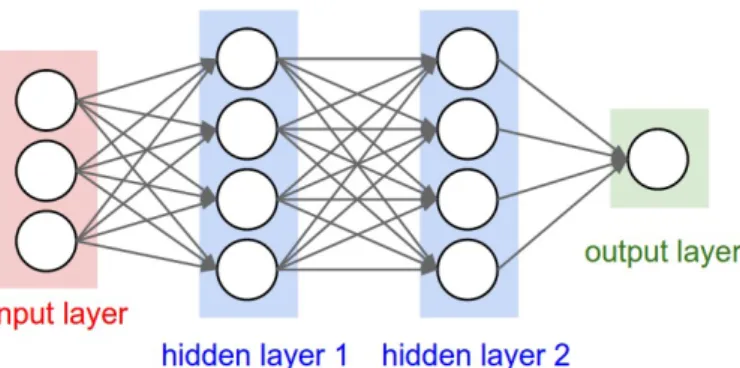
The quintessential example of neural networks is the feedforward network [60]. The feedforward network is a multi-layer neural network that performs computation iteratively from one layer to the next without passing back. The structure of a three-layer feedforward network is shown in Figure 1 [61]. The network is fully-connected, which means that neurons between adjacent layers are pairwise connected [61].
Figure 1: A simple three-layer feedforward neural network: the network contains one input layer, two hidden layers and one output layer. Each layer consists of multiple units, represented by circles [61].
The core of the neural network is the hidden layer which takes a weighted sum of its input and then apply a non-linear transformation to it [41]. The computation of feedforward networks proceeded according Equation 20. Here, x and y stands for the input and output vectors of the network separately, the superscript l represents thel-th layer,W(l)andb(l) refer to the weight matrix and bias term of thel-th layer,
respectively,σ(·)means the activation functions, and the capitalL is the number of layers in the network. Note that each hidden layer could apply distinctive activation
functions.
z(0) =x
z(l) =W(l)·z(l−1)+b(l)
a(l) =σ(z(l)) (20)
y=a(L)
The network shown in Figure 1 has a single output node and can perform binary classification if the activation function of the last layer is the sigmoid function. However, when trying to do a multi-class classification task, the softmax function would be a priority choice. The softmax function can output normalized vectors of real values that encode a probability distribution. Based on it, it is straightforward to assign the most likely category to an input vector. The softmax function is presented below: sof tmax(zi) = ezi Pd j=1ezj 1≤i≤d , (21)
where d is the number of categories, zi and zj represents for i-th and j-th entry of vectorz.
After knowing the structure of the feedforward neural network, the next step is to learn how to train the network. Training neural networks means to find wight matrices and bias terms (parameters of neural networks) that fits the training data most appropriately. From this aspect, neural networks were considered as supervised learning approaches. Therefore, we use the same method that is used in other supervised learning models to find the most likely parameters. The first step is to define a loss function, and then, we minimize the loss function using the gradient descent optimization algorithm.
However, performing gradient descent requires the knowledge of gradient of the loss function whose analytical expression is hard to get. The solution to this is an algorithm called error backpropagation. The method computes the derivatives of intermediate variables, such as z(l) and a(l) with respect to model parameters and then makes use of chain rule to obtain the derivative of the model loss L with respect to model parameters.
Finishing the model training and evaluation, we can utilize the trained neural net-works to make predictions. Before that, there are some practical techniques that we should pay attention to. Firstly, it is not allowed to initialize the gradient descent with all the weights and biases assigned the value 0, because doing this will make
hidden units symmetric and the model loses its non-linearity [60]. As a result, we have to initialize the parameters with small random numbers. Secondly, it is always helpful to fine-tune the hyper-parameters which are determined by the architecture designer, such as the number of hidden units and layers [41]. In addition, sometimes the architecture of neural networks we chose might be too complex to fit the data, which leads to the problem of overfitting. One technique that is popularly adopted to avoid overfitting is called dropout, which randomly drops some units and their connections from the network during training [41].
3.3.2 Neural network language model
The concept of applying neural networks in language modeling was first proposed in 2001 by Begino et al [51]. The goal of their work is to fight the curse of dimensionality of SLMs by learning a distributed representation for tokens. At the same time, the model learns a probability distribution of word sequences in terms of the token representations. The architecture of the neural language model is shown in Figure 2 [51].
Figure 2: The architecture of a probabilistic neural language model: the neural language model contains a embedding layer that is represented as Martix C, a hidden layer with tanh activation function, and an softmax output layer [51].
word into a feature vector of a predefined dimension. The resulting word vectors are concatenated as the input of the tanh hidden layer. Thereafter, the softmax layer maps the output vector of the hidden layer into a conditional probability distribution over words in the vocabulary V. If we set an input sequence w1w2..wT, a mapping functionCthat assigns feature vectors to words in V, and a functiongthat outputs the conditional probability distributionp(wt|w1..wt−1), the model can be formulated
mathematically in Equation 22.
p(wt|w1..wt−1)≈p(wt|wt−n+1..wt−1) =g(C(wt−1), ..., C(wt−n+1)) (22)
It was shown that neural language models surpass n-gram language models by a high margin [51, 56]. However, the model suffers from two major deficiencies: 1) it fails to deal with the sequence of varying lengths and, 2) it is impossible to capture important temporal properties of the language. To solve these problems, the recurrent neural networks (RNN) were adopt by researchers in computational linguistics.
3.3.3 Recurrent neural network based language model
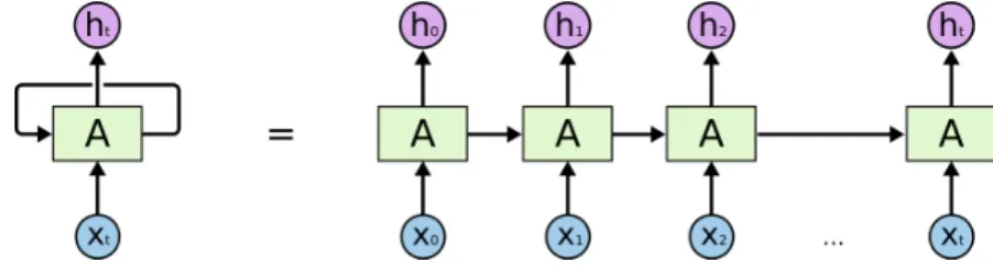
Unlike feedforward neural networks, the recurrent neural architecture can recursively process and leverage the information from the past when computing the current state, and therefore have been widely used for modeling sequential data. Particu-larly, RNNs have become a prominent choice for language modeling.
Figure 3: The structure of a general recurrent neural network: the left diagram depicts the structure of a general RNN, which can be unfolded into a chain diagram on the right side. An RNN contains a chunk of neural networks, A, which takesxt and the past hidden state ht−1 as input and outputs the current state ht [62].
Figure 3 [62] illustrates the structure of a general RNN. The loop represents the flow of information passing from one time step to the next. Mathematically, the computation of the RNN is based on Equation 23 [60, 63].
wheref(.)represents the activation function of the neural networkA, while matrices
W and U stand for the weight matrices for both inputxtand previous hidden state
ht−1 in the hidden layer. It should be noted that a softmax layer that maps the
output ht to a conditional probability distribution will be added when applying RNN into language modeling.
The intrinsic property of recurrence allows RNN to not only capture the temporal nature of language but to eliminate the limitation on the length of input sequences. This leads to incredible success in NLP [60]. However, despite the fact that RNN is supposed to learn the long-term dependencies between the previous and recent information, it was shown that the standard RNN is not capable of doing that as the sequence length increases due to the vanishing gradient problem [63]. As a result, the long short term memory (LSTM) network was proposed to overcome the issue.
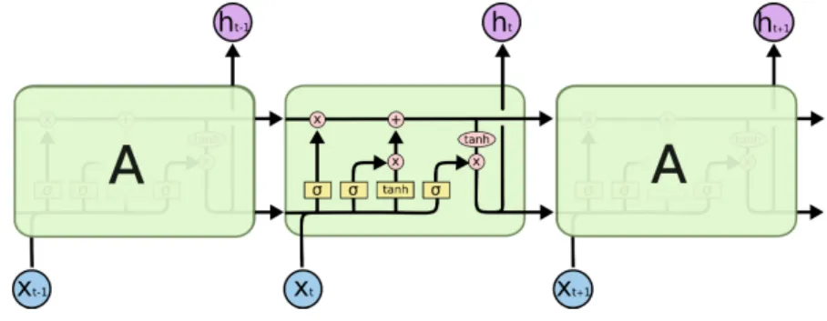
Figure 4: The structure of a LSTM network: the symbol of σ within a yellow box stands for the operation of passing a gate. These symbols represent the input gate, the forgetting gate, and the output gate from left to right [62].
LSTM shares the main concept from plain RNNs. As one of the most used variants of RNN, LSTM considered more about the way to process the memory of previous hidden states by adding three control gates: the input gate, the forgetting gate, and the output gate respectively. The diagram of LSTM is shown in Fig.4 [62].
Combined with a set of formulas of LSTM (Equation 24), we illustrate the process flow of an LSTM network here. Firstly, the states of three control gates are deter-mined by the linear combination of inputxt and the previous output ht−1. The use
of the sigmoid function (represented as σ) scaled all entries of gate states it, ft, ot into the range between 0 to 1. Subsequently, the current information, ˜ct, is com-puted byxtandht−1 with a tanh activation function, consistent with the calculation
in RNN. Most importantly, the current cell state is the linear combination of the weighted current and previous information,itc˜tandftc˜t−1. As the computation
suggests, the input gate controls what new information is supposed to be kept in the cell state and the forget gate decides what old information the network would like to abandon. As the final step, the cell state is put through a tanh function, which pushes the output values into the range between −1 and 1. Then, the result is multiplied by the output gate state ot that determines what information should be output [60, 62]. it=σ(Wixt+Uiht−1) ft=σ(Wfxt+Ufht−1) ot=σ(Woxt+Uoht−1) ˜ ct=tanh(Wcxt+Ucht−1) ct=itc˜t+ft˜ct−1 ht=ottanh(ct) (24)
Although the computation of LSTM is complicated, its way of storing and processing information is highly consistent with how human brains work [62]. As a result, LSTM has achieved huge success in challenging tasks of language processing, such as speech recognition and machine translation and, became the most popular choice of neural architectures for language modeling [60].
Because of the superior performance, researchers have created many variants of LSTM and employed them in language modeling. The AWD-LSTM (ASGD weight-dropped LSTM) is one of the most representative architectures among those variants [57]. AWD-LSTM adopts advanced regularization and optimization techniques to not only avoid overfitting caused by the high degree of complexity of LSTM but to achieve state-of-the-art results on benchmarks of language modeling [57]. Therefore, we chose the AWD-LSTM as the representative of a number of LSTM-based language models in our experiment.
It is worth mentioning that the bidirectional LSTM architecture is also used for building language models [58]. The bidirectional LSTM, as the name suggests, stands for a set of LSTM-based models that learn the conditional probability dis-tribution of possible next words given contexts from both left and right sides. It is suggested that these models benefit from the future information being provided and have achieved significant performance in various of NLP tasks such as senti-ment analysis even without fine-tuning [58]. Nevertheless, the bidirectional LSTM language models are not capable of generating text due to the lack of the right-hand context during generation. Here, we selected a representative bidirectional LSTM
architecture, contextual bi-LSTM [58], to perform our experiment.
3.3.4 Attention mechanism and the Transformer
In recent years, incredible progress has been made in language modeling, thanks to the introduction of the attention mechanism.
The concept of "attention" originated from the Seq2Seq (sequence-to-sequence) model which, as the name suggests, represents a group of models that transform the input sequence into another sequence [41]. The most intuitive example of the transformation is machine translation between multiple languages. A Seq2Seq model consists of an encoder that compresses the input sequence into a distributed context vector, and a decoder which transforms the context vector into the target sequence.
The earliest Seq2Seq models used RNNs for both encoder and decoder. According to what we learned about RNNs, the encoder will convert the input sequence into a fixed-length vector from which the decoder generates the output sequence. The limitation of the context vector is considered as a bottleneck that affects model performance. In 2015, Bahdanau et al. proposed the attention mechanism to deal with this issue [48].
Figure 5: The attention mechanism: the values, V, are weighted and summed up by attention-weights that are obtained through a set of operations on the queries,
The attention mechanism is used to search for a set of positions in the input sequence where the most relevant information is concentrated. More specifically, a set of alignment scores describing how relevant each input hidden state and output element are will be learned while training the model. Fig.5 depicts the process flow of the attention mechanism, in which the attention operation is considered as a retrieval process [64, 65]. Based on the Figure 5, the operations are formulated by Equation 25, wheredkis the dimension of matrixK and(a)represents the vector of attention-weights. Through model training, the most likely parameters of the softmax layer and possible middle layers can be obtained and then be used to calculate a vector that aligns attention score for each value inV [65].
a =sof tmax( QK T sqrt(dk) ) Attention(Q, K, V) =aV (25)
The attention mechanism makes better use of potential information of sequential data, and therefore achieved comparable performance on the task of English-to-French translation [48].
Subsequently, in 2017, a novel attention-based language model, the Transformer, was proposed by Ashish et al. [64]. This model dispenses with complex RNN archi-tectures entirely and is based solely on the attention mechanism. This architecture surpasses complicated RNN-based models on machine translation tasks and requires significantly less time to train. The structure of the Transformer is demonstrated in Figure 6 [64].
As shown in Figure 6, both encoder and decoder of the Transformer are stacked by six identical layers. Each layer in the encoder has two sub-layers that perform multi-head attention and vector transformation respectively. A residual connection is employed in each of the sub-layers. Different from each encoder layer, a middle sub-layer that performs multi-head attention over the output of the encoder stack is inserted in each decoder layer.
It should be noted that the incredible performance achieved by Transformer benefits from the use of a new technique called multi-head attention. Different from the standard attention mechanism, multi-head attention repeatedly applies the scaled dot-product attention (the standard attention) on linear projections ofQ, K, V mul-tiple times. This allows the system to learn the attention weights from different representations of Q, K, V, which yields better performance. Figure 7 shows the structure of multi-head attention, and multi-head attention is written as Equation
Figure 6: The structure of the Transformer: the stack on the left-side is the encoder while decoder is placed on the right [64].
26, where WiK, WiK, WiV are parameter matrices that are used to unify the dimen-sions of projections of matrices Q, K, V [64].
M ultiHead(Q, K, V) =Concat(head1, ..., headh)WO
headi =Attention(QWiK, KW K i , V W
V
i ) (26)
3.3.5 Pre-trained language models
It is worth mentioning that the great thing about the Transformer is not only its superior performance, but the fact that it has also led to the birth of two powerful pre-trained language models, BERT (2018, [17]) and GPT-2 (2019, [59]). BERT is a multi-layer bidirectional Transformer encoder. While GPT-2, the second version
Figure 7: Multi-Head Attention consists of several parallel scaled dot-product at-tention layers [64].
of the OpenAI Generative Pre-training Transformer (2018, [66]), is a multi-layer Transformer decoder. Both BERT and GPT-2 are pre-trained on a giant collection of free online corpora. BERT was pre-trained on the BooksCorpus (800M words) and English Wikipedia (2,500M words), while GPT-2 was pre-trained on around 40GB of Internet text [59, 17]. They have achieved significant performance on multiple downstream NLP tasks, such as question answering, textual entailment and sentiment analysis by simply fine-tuning [17, 66, 59].
Basically, the language model pre-training aims to transfer the pre-trained language representations to downstream tasks in order to ease the difficulty of solving chal-lenging NLP problems [17]. There are two strategies used by existing pre-trained language models: feature-based and fine-tuning. The most famous feature-based model is ELMo ((Embeddings from Language Models, 2018, [67]), which adopts pre-trained language representations on task-customized architectures and has sig-nificantly improved the model performance. The fine-tuning approaches, such as BERT and GPT-2, trained huge language models that can be reused by down-stream tasks with little changes in model architectures [17]. Here, we chose to use the fine-tuning based model to get rid of the high level of complexity of finding optimal model architectures required by the feature-based approaches.
lan-guage model on a giant collection of free online corpora at the first stage to capture the linguistic information. This step is performed in an unsupervised manner, which avoids the need for gathering a large labeled dataset. As the second step, the pre-trained language model is fine-tuned over a small task-customized dataset to ensure good performance on a specific task.
Figure 8: The architecture of the OpenAI GPT: the model contains a embedding layer, 12 blocks of the Transformer decoder, and a Softmax layer [66] .
The architecture of GPT is shown in Figure 8 [66]. The model takes embeddings of texts as input and outputs a distribution over the vocabulary after passing through 12 blocks of the Transformer decoder and a Softmax layer. As a supplement, the task-aware input transformations will be performed during the fine-tuning stage, in order to make sure the suitability of the pre-trained model for the target task [66].
Although it was demonstrated that GPT has incredible success in a wide range of benchmarks for natural language understanding, it may be limited by its uni-directional nature, which causes the ineffective utilization of the training data. Sev-eral months after the birth of GPT, a bi-directional pre-trained model, BERT, came out and beat its ancestor [17].
Instead of using the traditional method of training a language model, BERT adopts two auxiliary tasks: mask language modeling and next sentence prediction, to en-courage better bi-directional prediction and sentence-level understanding. After training, the pre-trained BERT is fine-tuned by adding an extra output layer to suits the target task. BERT has achieved new state-of-the-art results on multiple downstream tasks, such as question answering and language inference [17].
Subsequently, a much larger and powerful pre-trained language model, GPT-2, was proposed by Radford et al [59]. GPT-2 inherits the architecture from GPT and is 10 times larger than GPT with 1.5 billion parameters. At the same time, it was pre-trained on a more than 10 times larger dataset to void overfitting. GPT-2 achieves state of the art results on 7 out of 8 benchmarks in different NLP tasks, including Penn Tree Bank, WikiText-2, Winograd Schema Challenge, and so on, in a zero-shot setting – without any fine-tuning. This property makes GPT-2 prominent among pre-trained language models [59].
Our choice of pre-trained language models finally settled on GPT-2 due to its po-tential of performing well on multiple language understanding tasks in a zero-shot setting.
4
Methodology
We used an unsupervised ranking-based method to explore if language models can be used to measure the text readability and text quality.
Our method is based on two hypotheses: i) language models trained on a well-written corpus will be less perplexed on articles that are simple and well-well-written, ii) the more predictable the words in the article are, the more readable and well-written the article is.
Based on the hypotheses, we proposed two metrics: average per word perplexity and average likelihood ratio, that we thought can measure how well a language model predicts text, to assess text readability and text quality. Here, we investigated the following questions:
1. Whether the metrics correlate well with readability scores or quality scores that are assigned by human raters.
articles and therefore can be used to assess writing competence of articles.
To find the answer to the above questions, we performed multiple correlation ex-periments on various language models, such as bigram, LSTM, bidirectional LSTM and GPT-2. These language models were trained on the Guardian corpus, a British newspaper, that we thought is well-written. Further, we used three corpora, Newsela [4], OneStopEnglish [5] and Weebit [68] that are widely used in text readability studies, in order to verify the relation between text readability and the metrics. As for the study of text quality, we used the self-collected IELTS corpus and another ASAP corpus to measure the correlation between pre-assigned quality scores and the metrics.
In this chapter, the details of datasets and model architectures used in this thesis will be described in Chapter 4.1 and 4.2, respectively. Chapter 4.3 will demonstrate the intuitive derivation of the metrics, word perplexity and word ratio, followed by the introduction to the correlation coefficients that we used to evaluate our metrics in Chapter 4.4.
4.1
Dataset description
We used 6 corpora in total. The language models were trained using news arti-cles from The Guardian, a British newspaper. We assume that these artiarti-cles are well-written because they were written by journalists, who write for a living. Exper-iments for readability assessment were conducted on the Newsela, OneStopEnglish and WeeBit corpora, which are the three most popular datasets used for assessing readability and text simplification tasks. Besides, we adopted the IELTS corpus and the ASAP++ dataset to estimate the performance of text quality evaluation.
4.1.1 The Guardian Corpus
It is common for language models to be trained on English Wikipedia. However, as it has been criticized for the writing quality of Wikipedia articles [1], we instead decided to create our own corpus of well-written text. For this purpose, we downloaded news articles from The Guardian, a UK newspaper. Articles from newspapers are written by journalists, who are trained to write clearly and concisely. In addition, newspaper articles will have been checked by several editors for correctness and to achieve a consistent style prior to publication.
We crawled 20,000 news articles (May 12, 2019 - September 17, 2019) from four categories (news, culture, sport and lifestyle) of The Guardian’s website. Each cat-egory contains 5,000 articles (downloaded September 18th, 2019). Each article was pre-processed by removing non-ascii characters and setting text to lowercase. Sub-sequently, we shuffled the ordering of the articles and split the corpus into training, validation and test sets in the proportions, 80%, 10% and 10%, respectively.
4.1.2 The Newsela Corpus
The Newsela corpus contains articles intended for students of various age groups and is widely used to assess text complexity and to evaluate the reading ability of students [4]. Here, we used the latest version of Newsela (from January 9th, 2016), which contains 10,786 articles, each of which is supplemented by up to five simplified versions of the same article. Simplified articles were written by experienced editors in order to make them easier to understand for students at different grade levels. We filtered out non-English articles and deleted those that did not have corresponding simplified versions. Of the remaining 9,565 articles, 28 articles had 3 simplified versions, 1,840 had 4 simplified versions, and the remaining 42 had 5 simplified versions.
4.1.3 The OneStopEnglish Corpus
The OneStopEnglish corpus was created by Vajjala et al. in 2016 and became pub-licly available in 2018 for automatic readability assessment and text simplification tasks [5]. The dataset contains 567 articles from 2013-2016 from the OneStopEnglish website. As an English language learning resources website, the OneStopEnglish website is mainly aimed at second language learners. The articles on the website are sourced from The Guardian and have been rewritten by experienced teachers into three versions, namely advanced, intermediate and elementary. This means that the corpus contains 3 different versions of 189 articles.
4.1.4 The WeeBit Corpus:
The WeeBit corpus was first used in the study of second language readability clas-sification by Vajjala in 2012 [68]. The data was sourced from two websites: the Weekly Reader and BBC Bitesize, which are aimed at audiences of different ages. The articles from these two websites are merged and then divided into 5 categories
that correspond to the 7-8, 8-9, 9-10, 10-14, 14-16 age groups. Since there are mul-tiple broken files in the dataset, we did a series of pre-processing steps, including removing empty and duplicate files, deleting files that containing anomalous text, and fixing coding issues. At the same time, in order to balance the number of arti-cles in each category, we downsampled the group of age 14-16 which has the largest number of articles. In the end, we obtained a corpus that contains 3,096 articles.
4.1.5 The IELTS Corpus
We crawled 107 scored essays from the IELTS Academic test from IELT-Blog.com. The website provides various materials for students who aim to obtain good grades in IELTS Academic test. The IELTS academic test is a well-known English test among second language learners, especially among university students who desire to study in countries whose local language is English. The test consists of four parts: listening, speaking, reading and writing. As one of the hardest parts of the test, writing requires students to compose an essay of 250-350 words on a given topic. The grade ranges from 1 to 9, where band 9, the highest score, represents that the essay has a high degree of quality, while band 1 suggests that the essay uses very limited vocabulary and basically fails to convey any information.
Here, the 107 essays we used were scored from 5 to 9. The essay that has higher grade is considered to have better quality and be well-written. It should be noted that our dataset is imbalanced due to the limited access to scored essays of the IELTS test online.
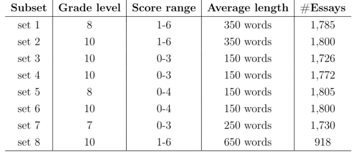
4.1.6 The ASAP Dataset
The Automated Student Assessment Prize’s dataset (ASAP) was first introduced by Shermis and Burstein in 2013 for automated essay evaluation [19]. After that, ASAP is widely used for evaluating the score of essays and have become a benchmark of automated essay scoring (AES).
The original ASAP dataset consists of 8 subsets that contains essays written over 8 prompts (given topics). The whole dataset includes 12,978 essays that contain 150 -500 words. Each essay was double-graded by at least one and up to three proficient evaluators based on the overall quality of an essay. However, as our work aims to prove the relation between metrics we proposed and text quality which relates to a variety of aspects to consider, we assumed that the overall score is not enough for our use. Fortunately, in 2018, Mathias and Bhattacharyya [69] supplemented the
![Figure 2: The architecture of a probabilistic neural language model: the neural language model contains a embedding layer that is represented as Martix C, a hidden layer with tanh activation function, and an softmax output layer [51].](https://thumb-us.123doks.com/thumbv2/123dok_us/9050423.2803015/25.892.242.690.574.934/architecture-probabilistic-language-language-contains-embedding-represented-activation.webp)
![Figure 5: The attention mechanism: the values, V , are weighted and summed up by attention-weights that are obtained through a set of operations on the queries, Q, and the keys, K [64].](https://thumb-us.123doks.com/thumbv2/123dok_us/9050423.2803015/29.892.369.529.622.951/figure-attention-mechanism-weighted-attention-weights-obtained-operations.webp)
![Figure 6: The structure of the Transformer: the stack on the left-side is the encoder while decoder is placed on the right [64].](https://thumb-us.123doks.com/thumbv2/123dok_us/9050423.2803015/31.892.274.655.108.681/figure-structure-transformer-stack-encoder-decoder-placed-right.webp)
![Figure 7: Multi-Head Attention consists of several parallel scaled dot-product at- at-tention layers [64].](https://thumb-us.123doks.com/thumbv2/123dok_us/9050423.2803015/32.892.335.601.97.467/figure-multi-attention-consists-parallel-scaled-product-tention.webp)
![Figure 8: The architecture of the OpenAI GPT: the model contains a embedding layer, 12 blocks of the Transformer decoder, and a Softmax layer [66] .](https://thumb-us.123doks.com/thumbv2/123dok_us/9050423.2803015/33.892.358.578.275.698/figure-architecture-openai-contains-embedding-transformer-decoder-softmax.webp)