A distributed brain network predicts
general intelligence from resting-state
human neuroimaging data
Julien Dubois1,4, Paola Galdi5, Lynn K. Paul1,3 , Ralph Adolphs1,2,3
1 Division of Humanities and Social Sciences, California Institute of Technology, Pasadena CA
91125, USA
2 Division of Biology and Biological Engineering, California Institute of Technology, Pasadena
CA 91125, USA
3 Chen Neuroscience Institute, California Institute of Technology, Pasadena CA 91125, USA 4 Department of Neurosurgery, Cedars-Sinai Medical Center, Los Angeles, CA 90048, USA 5 Department of Management and Innovation Systems, University of Salerno, Fisciano, Salerno,
Italy
Correspondence: Julien Dubois
Department of Neurosurgery
Cedars-Sinai Medical Center, Los Angeles, CA 90048 [email protected]
Abstract
Individual people differ in their ability to reason, solve problems, think abstractly, plan and learn. A reliable measure of this general ability, also known as intelligence, can be derived from scores across a diverse set of cognitive tasks. There is great interest in understanding the neural underpinnings of individual differences in intelligence, since it is the single best predictor of long-term life success, and since individual differences in a similar broad ability are found across animal species. The most replicated neural correlate of human intelligence to date is total brain volume. However, this coarse morphometric correlate gives no insights into
mechanisms; it says little about function. Here we ask whether measurements of the activity of the resting brain (resting-state fMRI) might also carry information about intelligence. We used the final release of the Young Adult Human Connectome Project dataset (N=884 subjects after exclusions), providing a full hour of resting-state fMRI per subject; controlled for gender, age, and brain volume; and derived a reliable estimate of general intelligence from scores on multiple cognitive tasks. Using a cross-validated predictive framework, we predicted 20% of the variance in general intelligence in the sampled population from their resting-state fMRI data. Interestingly, no single anatomical structure or network was responsible or necessary for this prediction, which instead relied on redundant information distributed across the brain.
Introduction
Most psychologists agree that there is, in addition to specific cognitive abilities, a very general mental capability to reason, think abstractly, solve problems, plan, and learn across domains [1]. This ability, intelligence, does not refer to a person’s sheer amount of knowledge but rather to their ability to recognize, acquire, organize, update, select and apply this knowledge [2], to reason and make comparisons [3]. There are large and reliable individual differences in intelligence across species: some people are smarter than others, and some rats are smarter than others [4].
What’s more, these differences matter. Intelligence is one of the most robust predictors of conventional measures of educational achievement [5], job performance [6], socio-economic success [7], social mobility [8], health [9] and longevity [10,11]; and as life becomes increasingly complex, intelligence may play an ever increased role in life outcome [2]. Despite this
overwhelming convergence of evidence for the construct of “intelligence” there is considerable debate about what it really is, how best to measure it, and in particular what predictors and mechanisms for it we could find in the brain.
Measuring intelligence: the structure of cognitive abilities
Although apparent in its consequences in everyday life, this is not how intelligence has been operationalized psychometrically. Instead, it is tied to performance on very specific tests, or factor analyses derived from tests. Intelligence tests are among the most reliable, and valid, of all psychological tests and assessments [1]. Psychologists are so confident in the psychometric properties of intelligence tests that, almost 100 years ago, Edwin G. Boring infamously wrote: “Intelligence is what the tests test.” [12].
A comprehensive modern intelligence assessment (such as the Wechsler Adult Intelligence Scale, Fourth Edition or WAIS-IV [13]) comprises tasks that assess several aspects of intelligence: some assess verbal comprehension (e.g. word definition, general knowledge, verbal reasoning), some assess visuo-spatial reasoning (e.g., puzzle construction, matrix reasoning, visual perception), some assess working memory (e.g., digit span, mental arithmetic, mental manipulation), and some some assess mental processing speed (e.g., reaction time for detection). The scores on all of these tasks are tallied and compared to a normative,
age-matched sample to calculate a standardized Full Scale Intelligence Quotient (FSIQ) score. One of the most important findings in intelligence research is that performances on all these seemingly disparate tasks -- and many other cognitive tasks -- are positively correlated - individuals who perform above average on, say, visual perception, also tend to perform above average on, say, word definition. Spearman [14] discovered this phenomenon and described it as the positive manifold, and since then it has been described in a number of species [15]. To explain this empirical observation, he posited the existence of a general factor of intelligence, the ‘g-factor’, or simply ‘g’, which no single task can perfectly measure, but which can be derived
from performance on several cognitive tasks through factor analysis. The g-factor explains around half of people’s intellectual differences [16] and shows good reliability across sets of cognitive tasks [17].
The empirical observation of the positive manifold is well-established [18] (it is sometimes referred to as the most replicated result in all of psychology [19]). The descriptive value of Spearman’s g is beyond doubt, however its interpretation -- that psychometric g reflects a general aspect of brain functioning -- was challenged early on [20] and remains a topic of
debate to this day among intelligence researchers [21–23]. The leading alternative theory posits that each cognitive test involves several mental processes, and that the sampled mental
processes overlap across tests; in this situation, performance on all tests appears to be positively correlated. The common factor, in this framework, is a consequence of the positive manifold, rather than its cause. The most recent formulation of this view was coined “Process Overlap Theory” [19], and the response it received demonstrates the division in the field [24]. The main issue, in this ongoing debate, is that there is no statistical means of distinguishing between alternate theories on the basis of the psychometric data alone [22]. Thus the
interpretation of g as general intelligence may be sufficient, but it is not a necessary explanation of the positive manifold.
Beyond the debate on the nature of the g-factor, the structure of intelligence is often described in terms of broad abilities, the exact nature of which is also still debated. Prominent theories provide differing descriptions of those broad abilities. The Cattell–Horn–Carroll (CHC) theory [25] recognizes 9 broad domains of ability: Gf (fluid reasoning), Gc (comprehension/knowledge), Gv (visual-spatial processing), Ga (auditory processing), Gsm (short-term memory), Glr
(long-term storage and retrieval), Gs (cognitive processing speed), Gq (quantitative knowledge), and Grw (reading and writing). At the root of the CHC theory is the distinction between a “fluid” intelligence, which reflects the capacity to reason and solve problems without using knowledge; and a “crystallized” intelligence, which reflects the ability to use knowledge and experience [26]. The main contending theory is the verbal–perceptual–image rotation (VPR) theory [27,28], which simply posits three broad abilities and does not distinguish whether prior knowledge is used or not. There is one major finding that supports a distinction between fluid and crystallized intelligence [29]: though the two are highly correlated, they change differentially with age [30,31]. Fluid intelligence starts declining around age 25, whereas crystallized intelligence increases until about age 50 and then shows little decline.
The search for biological substrates of intelligence
Differential psychology -- the psychological discipline that studies individual differences between people -- has three main aims: to describe the trait of interest accurately, to establish its impact in real life, and to understand its aetiology, including its biological basis [32]. Much headway has been made with respect to the first two aims for intelligence, as described above. The third aim, despite much effort, has remained elusive.
Individual differences in intelligence are relatively stable: one of the best predictors of
intelligence in old age is - perhaps unsurprisingly - intelligence in childhood [33]. Intelligence has a strong genetic component; heritability estimates from twin studies range between .20 (for
children) and .80 (for adults) [5] (see also [34] for data from adoption studies). Genome-Wide Association Studies (GWAS) yield similar heritability estimates [35], and suggest that
intelligence is highly polygenic (no single gene accounts for a large fraction of the variance) [36,37].
While high heritability points to genes as an undeniable distal cause of intelligence differences, the proximal cause for individual differences in cognitive ability is to be found in brain function. Arguably, studying the proximal cause may yield more direct insight about the actual
mechanisms of intelligence than genetic studies have so far. Since intelligence is a relatively stable trait, one might reason that its aetiology should be found in stable aspects of brain function, and hence also predicted by aspects of brain structure. Most of the data on the neural basis of intelligence comes from neuroimaging and from lesion studies. There are several in-depth reviews of the neurobiological substrates of intelligence, to which the interested reader is referred for a more complete treatment [32,38–40]. Kievit et al. [41] recently described the current state of the neuroscience of intelligence as “an embarrassment of riches” -- a plethora of neuroimaging-derived properties of the brain, structural and functional, have been linked to intelligence over the years. However, many of these claims may not replicate, due to methodological concerns such as data overfitting in small subject samples. Here we briefly highlight some key results to help set the stage for our study.
It is worth noting, from the outset, that the naive search for a simple neurobiological correlate of intelligence faces a major theoretical hurdle, which is best understood through analogy [41]. Imagine a researcher trying to find the biological basis of the construct of “physical fitness”. If they search for a single physical property, they would likely fall short of their goal. Indeed, physical fitness is a composite of several physical properties (cardiorespiratory endurance, muscular strength, muscular endurance, body composition, flexibility), and cannot be equated with any single one, or even any specific combination of these factors. It is very likely that intelligence is of a similar composite nature, as suggested by genetic data [36]. Furthermore, individuals may score identically on an IQ test by using different cognitive strategies, or different brain structures [32]. This is an important picture to hold in mind as one searches for neural correlates of intelligence.
Structural studies
The best replicated brain correlate of intelligence is a fairly simple one: size matters [42]. People who score higher on IQ tests tend to also have bigger brains, as assessed nowadays using total brain volume derived from structural MRI scans; the correlation coefficient is about r=0.24 according to the meta-analytical estimates [43] (or maybe as much as r=0.40 [44]). Initial correlation estimates using small sample sizes were as high as 0.51 [45], and were revised down multiple times [46]. The volume of gray-matter seems slightly more strongly related to intelligence than the volume of white matter [47].
Finer-grained measures, such as cortical thickness or volume of specific regions across the whole brain, have also been shown to correlate positively with intelligence [47], though usually with small sample sizes which may undermine statistical power and replicability.
Recent studies with larger sample sizes have reported associations between intelligence and white matter tract structure (from diffusion imaging [48,49]) as well as white matter integrity (volume of white matter hyperintensities, number of microbleeds, number of iron deposits) [50]; a combination of these with brain volume and cortical thickness has been shown to account for as much as 20% of the variance in g [51]. The role of white matter is further corroborated by several MR spectroscopy studies which find a relationship between N-acetyl aspartate, a metabolite of the oligodendrocytes that constitute the myelin sheath [52], and IQ scores. Neuroimaging studies remain correlative in nature, and causal inference is limited. Lesion studies in humans are an opportunity to establish causation [53], although they come with their own set of limitations [54]. A recent study using a large sample of patients (N=241) used voxel-based lesion mapping and found specific lesion-deficit relationships for the g-factor and several broad ability domains, in frontal and parietal cortices [55].
Functional studies
Extant functional neuroimaging studies (using EEG, PET, rCBF and fMRI) have been
summarized as supporting the notion that intelligence is a network property of the brain, related to neural efficiency [38,56]. While this may generally be correct, foundational studies had very low sample sizes [56], and so did a recent study making a similar claim using graph analysis in N=19 subjects [57]. More recent, better powered studies have found correlations between intelligence and the global connectivity of a small region in lateral prefrontal cortex (N=78) [58]; the nodal efficiency of hub regions in the salience network (N=54) [59]; the modularity of frontal and parietal networks (N=309) [60]; and several other seemingly disparate reports.
A neurobiological model of intelligence
A 2007 review of existing structural and functional studies lead to the Parieto-Frontal Integration Theory (P-FIT) of intelligence [38], regarded as “the best available answer to the question of where in the brain intelligence resides” [32]. There aren’t many detractors of the P-FIT model, yet it is a very generic model, and falls short of a mechanistic understanding. Because the brain regions discussed in the model include most of the cortex, it seems difficult to falsify the theory experimentally -- leaving most studies little choice but to “generally support” the P-FIT model.
The current study
Current literature on the fMRI-derived substrates of intelligence suffers from the same caveats as most fMRI-based individual differences research to date [61]: small sample sizes, and lack of out-of-sample generalization. A predictive framework was first used in a recent study [62], which found that fluid intelligence could be predicted from functional connectivity matrices in an early release (N=118) of the Human Connectome Project (HCP) dataset [63], with a correlation rLOSO=0.50 between observed and predicted scores (the LOSO subscript denotes the use of a leave-one-subject-out cross-validation framework). Since this early report, the authors revised the effect size down to rLOSO=0.22 using later data releases (N=606) [64]. Recent work in our
group, in which we further control for confounding effects of age, gender, brain size and motion, as well as use a leave-one-family-out cross-validation framework (LOFO) instead of the original leave-one-subject-out framework (thus accounting for the family structure of the HCP dataset), further revised the effect size down to about rLOFO=0.09 using methods matched as closely as possible to the original study [62]; yet, using improvements including better inter-subject alignment and multivariate modeling, we found rLOFO=0.263 (N=884) [65]. Note that this effect size is comparable to recent estimates of the relationship between brain size and intelligence [43]. Though the explained variance is small, it would in fact fall around the 65th percentile of
correlations observed in individual differences research [66] (with the caveat that rLOFO correlation is derived from a cross-validation procedure, which breaks the assumption of independence between individual data points).
According to recent guidelines [44], the assessment of general intelligence with HCP’s 24-item Progressive Matrices would be considered of “fair” quality (1 test, 1 cognitive dimension, testing time less than 19 minutes), and would be expected to correlate with general intelligence in the range 0.50 to 0.71. This rather low measurement quality of intelligence itself is likely to
attenuate the magnitude of the relationship between neural data and general intelligence. Fortunately, there are several other measures of cognition in the HCP, which we here decided to leverage to derive a better estimate of general intelligence -- one that would meet criteria for an “excellent” quality measurement (more than 9 tests, more than 3 dimensions, testing time more than 40 minutes), and thus be expected to correlate with the general factor of intelligence above 0.95.
Our main aims in this study were to: i) predict an excellent estimate of general intelligence from resting-state functional connectivity in a large sample of subjects from the HCP; ii) depending on the success of i), gain some anatomical insight on which functional connections matter for these predictions. The current study paves the way for a reliable neuroimaging-based science of intelligence differences (large sample size; predictive framework; valid, reliable psychometric construct).
Methods
Many of the methods, in particular the preprocessing of fMRI data and the predictive analyses, were developed and described in our recent publication [65]. Consequently, some sections here were reproduced verbatim from the previous paper.
Dataset
We used data from a public repository, the 1200 subjects release of the Human Connectome Project (HCP) [63]. The HCP provides MRI data and extensive behavioral
assessment from almost 1200 subjects. Acquisition parameters and “minimal” preprocessing of the resting-state fMRI data is described in the original publication [67]. Briefly, each subject underwent two sessions of resting-state fMRI on separate days, each session with two separate 15 minute acquisitions generating 1200 volumes (customized Siemens Skyra 3 Tesla MRI
scanner, TR = 720 ms, TE = 33 ms, flip angle= 52°, voxel size = 2 mm isotropic, 72 slices, matrix = 104 x 90, FOV = 208 mm x 180 mm, multiband acceleration factor = 8). The two runs acquired on the same day differed in the phase encoding direction, left-right and right-left (which leads to differential signal intensity especially in ventral temporal and frontal structures). The HCP data was downloaded in its minimally preprocessed form, i.e. after motion correction, B0 distortion correction, coregistration to T1-weighted images and normalization to MNI space.
Cognitive ability tasks
Previous studies of the neural correlates of intelligence in the HCP [62,64] have relied on the number of correct responses on form A of the 24(+3 bonus)-item Penn Matrix Reasoning Test (PMAT), a test of non-verbal reasoning ability which can be administered in under 10 minutes (mean=4.6, std= 3 min; [68]), and is included in the University of Pennsylvania Computerized Neurocognitive Battery (Penn CNB, [69–71]). The PMAT is designed to parallel many of the psychometric properties of the Raven’s Standard Progressive Matrices test (RSPM, originally published in 1938), which comprises 60 items [72]. A computerized version of RSPM takes approximately 17 minutes to administer [73], which is too long for large-scale studies requiring an efficient assessment of all major neurocognitive domains. Bilker and colleagues developed an abbreviated 9-item version of the RSPM test which achieves similar item- and test-level characteristics to 60-item based scores, with an administration time of about 4 minutes [74]. This paved the way for the development of the computerized, adaptive PMAT test, whose items were designed from scratch to have similar psychometric characteristics as RSPM items, while limiting learning effects and expanding the representation of the abstract reasoning construct (Ruben Gur, personal communication).
Assessment of cognitive ability in the HCP [75] also includes several tasks from the Blueprint-funded NIH Toolbox for Assessment of Neurological and Behavioral function
(http://www.nihtoolbox.org), as well as other tasks from the Penn computerized neurocognitive battery [70]. These other tasks can be leveraged to derive a better measure of the general intelligence factor [44]. We included all cognitive tasks listed in the HCP Data Dictionary, except for: i) the delay discounting task, which is not a measure of ability (i.e. there is not a correct response); and ii) the Short Penn Continuous Performance Test which is about sustained attention rather than cognitive ability, and whose distribution departed too much from normality (data not shown) . Our initial selection thus consisted of 10 tasks, which are listed in Table 1
along with a brief description (the descriptions are copied almost word for word from the HCP Data Dictionary). When several outcome measures were available for a given task, we selected the one that best captured ability; when both age-adjusted and unadjusted scores were
available, we included the unadjusted scores. Though some of the NIH toolbox scores combine accuracy and reaction time, we only considered accuracies for the Penn CNB tasks (to avoid confounding ability and processing speed; but, see [71]).
Table 1. List of cognitive measures included in our analyses.
Subject selection
The total number of subjects in the 1200-subject release of the HCP dataset is N=1206. We applied the following criteria to include/exclude subjects from our analyses (listing in
parentheses the HCP database field codes). i) Complete neuropsychological datasets. Subjects must have completed all relevant neuropsychological testing (PMAT_Compl=True,
NEO-FFI_Compl=True, Non-TB_Compl=True, VisProc_Compl=True, SCPT_Compl=True,
IWRD_Compl=True, VSPLOT_Compl=True) and the Mini Mental Status Exam
(MMSE_Compl=True). Any subjects with missing values in any of the tests or test items were discarded. This left us with N = 1183 subjects.ii) Cognitive compromise. We excluded subjects with a score of 26 or below on the MMSE, which could indicate marked cognitive impairment in this highly educated sample of adults under age 40 [76]. This left us with N =1181 subjects (638 females, 28.8 +/- 3.7 y.o., range 22-37 y.o). This is the sample of subjects available for factor analyses.
Furthermore, iii) subjects must have completed all resting-state fMRI scans
excluded subjects with a root-mean-squared frame-to-frame head motion estimate
(Movement_Relative_RMS.txt) exceeding 0.15mm in any of the 4 resting-state runs (threshold similar to [62]). This left us with the final sample of N = 884 subjects (475 females, 28.6 +/- 3.7 y.o., range 22-36 y.o.) for predictive analyses based on resting-state data.
Deriving the general factor of intelligence,
g
There are several methods in the literature to derive a general factor of intelligence from scores on a set of cognitive tasks. The simplest consists in using a standardized sum score composite -- simply summing the standardized scores from all selected cognitive tasks. This is the conventional approach when all scores come from a well-validated battery. However, since we are here including scores from two different cognitive batteries (NIH toolbox and Penn CNB), we sought to characterize the structure of cognitive abilities in our sample using factor analysis, and then derive the scores for the general factor. We conducted an exploratory factor analysis (EFA), specifying the bi-factor model of intelligence -- a common factor g which loads on all test scores, and several group factors that each load on subsets of the test scores; all latent factors are orthogonal to one another -- using the psych (v1.7.8) package [77] in R (v3.4.2). We
specifically used the omega function, which conducts a factor analysis (with maximum likelihood estimation) of the data set, rotates the factors obliquely (using “oblimin” rotation), factors the resulting correlation matrix, then does a Schmid-Leiman transformation [78] to find general factor loadings. Model fit is assessed using several commonly used statistics in factor analysis [79]: the Comparative Fit Index (CFI; should be as close to 1 as possible; values >0.95 are considered a good fit); the Root Mean Squared Error of Approximation (RMSEA; should be as close to 0 as possible; values <0.06 are considered a good fit); the Standardized Root Mean Squared Residual (SRMR; should be as close to 0 as possible; values <0.08 are considered a good fit); and the Bayesian Information Criterion (BIC; better models have lower values, can be negative). Factor scores can be derived using different methods [80], for example the
regression method. This approach mimics the one taken by [55]. It is however usually preferable to derive scores from a confirmatory factor analysis (CFA). The main difference between EFA and CFA is that in EFA, observed task scores are allowed to cross-load freely on several group factors, while in CFA such cross-loadings can be forbidden. For the purpose of deriving the general factor of intelligence, there is little difference between using CFA and EFA in practice; we conducted a CFA using the lavaan (v0.5-23.1097) package [81] in R to verify this (see
Supplementary Material).
Assessment and removal of potential confounds
We computed the correlation of the general factor of intelligence g with Gender (HCP variable: Gender), Handedness and Age (restricted HCP variables: Handedness, Age_in_Yrs). We also looked for differences in g in our subject sample with variables that are likely to affect FC matrices, such as brain size (we used FS_BrainSeg_Vol), motion (we computed the sum of framewise displacement in each run), and the multiband reconstruction algorithm which
changed in the third quarter of HCP data collection (fMRI_3T_ReconVrs). We then used multiple linear regression to regress these variables from g scores and remove their confounding effects.
Note that we do not control for differences in cortical thickness and other morphometric features, which have been reported to be correlated with intelligence (e.g. [82]). These likely interact with FC measures and should eventually be accounted for in a full model, yet this was deemed outside the scope of the present study.
Data preprocessing
Resting-state data must be preprocessed beyond “minimal preprocessing”, due to the presence of multiple noise components, such as subject motion and physiological fluctuations.
Several approaches have been proposed to remove these noise components and clean the
data, however the community has not yet reached a consensus on the “best” denoising pipeline for resting-state fMRI data [83–86]. Most of the steps taken to denoise resting-state data have limitations, and it is unlikely that there is a set of denoising steps that can completely remove noise without also discarding some of the signal of interest. Categories of denoising operations that have been proposed comprise tissue regression, motion regression, noise component regression, temporal filtering and volume censoring. Each of these categories may be implemented in several ways. There exist several excellent reviews of the pros and cons of various denoising steps [84,87–89].
We recently explored the effects of several preprocessing pipeline on the prediction of personality factors and PMAT scores in the HCP dataset [65]. Here we adopt a preprocessing pipeline which was found to perform well in that study. The pipeline reproduces as closely as possible the strategy described in [62] and consists of seven consecutive steps: 1) the signal at each voxel is z-score normalized; 2) using tissue masks, temporal drifts from cerebrospinal fluid (CSF) and white matter (WM) are removed with third-degree Legendre polynomial regressors; 3) the mean signals of CSF and WM are computed and regressed from gray matter voxels; 4) translational and rotational realignment parameters and their temporal derivatives are used as explanatory variables in motion regression; 5) signals are low-pass filtered with a Gaussian kernel with a standard deviation of 1 TR, i.e. 720ms in the HCP dataset; 6) the temporal drift from gray matter signal is removed using a third-degree Legendre polynomial regressor; 7) global signal regression is performed. These operations were performed using an in-house, Python (v2.7.14)-based pipeline (mostly based on open source libraries and frameworks for scientific computing, including SciPy (v0.19.0), Numpy (v1.11.3), NiLearn (v0.2.6), NiBabel (v2.1.0), Scikit-learn (v0.18.1) [90–94]).
Inter-subject alignment, parcellation, and functional connectivity
matrix generation
We use surface-based multi-modally aligned cortical data (MSM-All [95]), together with a parcellation that was derived from this data using an objective semi-automated neuroanatomical
approach [96]. The parcellation has 360 nodes, 180 for each hemisphere. These nodes can be attributed to the major resting state networks [97] (Figure 4a).
Time series extraction simply consisted in averaging data from vertices within each parcel, and matrix generation in pairwise correlating parcel time series (Pearson correlation coefficient). We concatenated time series across runs to derive average FC matrices (REST1: from concatenated REST1_LR and REST1_RL time series; REST2: from concatenated
REST2_LR and REST2_RL time series; REST12: from concatenated REST1_LR, REST1_RL, REST2_LR and REST2_RL time series).
There are (360 * 359)/2 = 64620 undirected edges in a network of 360 nodes. This is the dimensionality of the feature space for prediction.
Prediction models
We use a univariate feature filtering approach to reduce the number of features, discarding edges for which the p-value of the correlation with the behavioral score is greater than a set threshold, for example p<0.01 (as in [62]).We then use Elastic Net regression to learn the relationship with behavior. Elastic Net is a regularized regression method that linearly combines L1- (lasso) and L2- (ridge) penalties to shrink some of the regressor coefficients toward zero, thus retaining just a subset of features. The lasso model performs continuous shrinkage and automatic variable selection simultaneously, but in the presence of a group of highly correlated features, it tends to arbitrarily select one feature from the group. With high-dimensional data and few examples, the ridge model has been shown to outperform lasso; yet it cannot produce a sparse model since all the predictors are retained. Combining the two approaches, elastic net is able to do variable selection and coefficient shrinkage while retaining groups of correlated variables. Here however, based on preliminary experiments and on the fact that it is unlikely that just a few edges contribute to prediction, we fixed the L1 ratio (which weights the L1- and L2- regularizations) to 0.01, which amounts to almost pure ridge regression. We used 3-fold nested cross-validation (with balanced “classes”, based on a partitioning of the training data into quartiles) to choose the alpha parameter (among 50 possible values) that weighs the penalty term.
Cross-validation scheme
In the HCP dataset, several subjects are genetically related (in our final subject sample there were 410 unique families). To avoid biasing the results due to this family structure (e.g., perhaps having a sibling in the training set would facilitate prediction for a test subject, if both intelligence and functional connectivity are heritable), we implemented a leave-one-family-out cross-validation scheme for all predictive analyses.
Statistical assessment of predictions
Several measures can be used to assess the quality of prediction. A typical approach is to plot observed vs. predicted values (rather than predicted vs. observed [98]). The Pearson
correlation coefficient between observed scores and predicted scores is often reported as a measure of prediction (e.g. [62]), given its clear graphical interpretation. However, in the context of cross-validation, it is incorrect to square this correlation coefficient to obtain the coefficient of determination R2, which is often taken to reflect the proportion of variance explained by the
model [99]; instead, the coefficient of determination R2 should be calculated as:
R
2= −
1
(1) ∑n i = 1 ( yi − yi )2 ∑n i = 1( yi − y ) ︿ i 2where n is the number of observations (subjects), y is the observed response variable, y̅ is its mean, and ŷ is the corresponding predicted value. Equation (1) therefore measures the size of the residuals from the model compared with the size of the residuals for a null model where all of the predictions are the same, i.e., the mean value y̅. In a cross-validated prediction context, R2 can actually take negative values (in cases when the denominator is larger than the
numerator, i.e. when the sum of squared errors is larger than that of the null model)! Yet another, related statistic to evaluate prediction outcome is the Root Mean Square Deviation (RMSD), defined in [98] as:
R
MSD
=
(2)√
1 n − 1∑
n i = 1(
y
i−
y
︿)
i 2RMSD as defined in (2) represents the standard deviation of the residuals. To facilitate interpretation, it can be normalized by dividing it by the standard deviation of the observed values:
(3)RMSD
n
=
√
1 n − 1 ∑ n i = 1 ( yi − yi)2√
1 n − 1 ∑ n i = 1 ( yi − y︿ )i 2=
√
∑n i = 1 ( yi − yi )2 ∑n i = 1( yi − y ) ︿ i 2=
√
1
−
R
2 nRMSD thus has a very direct link to R2 (3); it is interpretable as the average deviation of eachpredicted value to the corresponding observed value, and is expressed as a fraction of the standard deviation of the observed values.
In a cross-validation scheme, the folds are not independent of each other. This means that statistical assessment of the cross-validated performance using parametric statistical tests is problematic [100,101]. Proper statistical assessment should thus be done using permutation testing on the actual data. To establish the empirical distribution of chance, we ran our
predictive analysis using 1000 random permutations of the scores (shuffling scores randomly between subjects, keeping everything else exactly the same, including the family structure).
Results
A general factor accounts for 58% of the covariance structure of
cognitive tasks in the HCP sample
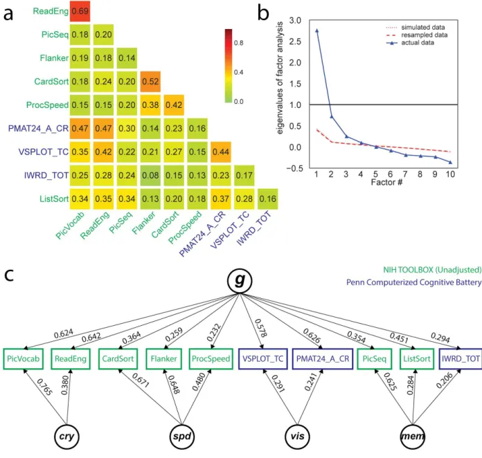
All selected cognitive task scores (Table 1) correlate positively with one another, as expected from the well-known positive manifold (Figure 1a). A parallel analysis suggests an underlying 4-factor structure (Figure 1b). An exploratory bifactor analysis with a general factor g
and 4 group factors fits the data very well (CFI=0.990; RMSEA=0.0311; SRMR=0.0201;
BIC=-0.519), much better than a single factor model (CFI=0.719; RMSEA=0.1398; SRMR=0.0887; BIC=591.172). The solution is depicted in Figure 1c. The four factors can naturally be interpreted as: 1) Crystallized Ability [cry] (PicVocab_Unadj + ReadEng_Unadj); 2) Processing Speed [spd] (CardSort_Unadj + Flanker_Unadj + ProcSpeed_Unadj); 3) Visuospatial Ability [vis]
(PMAT24_A_CR + VSPLOT_TC); and 4) Memory [mem] (IWRD_TOT + PicSeq_Unadj + ListSort_Unadj).
Across all cognitive task scores, the general factor accounts for 58.5% of the variance (coefficient omega_hierarchical ωh [102–104]), while group factors account for 18.2% of the variance (with 15.5% of the variance unaccounted for). Another important metric is coefficient omega_subscale ωs[105] which quantifies the reliable variance across the tasks accounted for by each subscale, beyond that accounted for by the general factor; we find ωscry=38.7%,
ωsspd=57.4%, ω
svis=9.9% and ωsmem=27.8%. While some of these subscale factors account for a
substantive proportion of the variance across their respective tasks, their measurement quality is at most fair [44] due to the limited number of constituent tasks; thus we choose to focus on the general factor g only.
Factor scores are indeterminate, and several alternate methods exist to derive them from a structural model [80]. To avoid this issue, most researchers prefer to remain in latent space for further analyses [41]. However, for subsequent analyses we require factor scores for g, which we derive using regression-based weights (“Thurstone” method).
We compare the general factor score derived from this exploratory factor analysis (EFA) with a simple composite score consisting of the sum of standardized observed test scores. As expected, we find that the simple composite score correlates highly with the EFA-derived g (r=0.91).
Though deriving factor scores from an EFA is often done by empirical researchers [106], it is theoretically preferable to use a confirmatory factor analysis (CFA) framework. A major difference is that a CFA model typically restricts cross-loadings (an observed variable loading on several latent factors), while the EFA allows them; this can reduce the size of the g factor in the EFA. We conduct a CFA (see Supplementary Material), and find that the g factor extracted from the CFA model correlates almost perfectly with the g factor extracted from the EFA model (r=.99). Therefore, we simply proceed with the EFA-derived g-factor in the following (in keeping with previous literature [55]).
Figure 1.Exploratory factor analysis of select cognitive tasks (Table 1) in the Human
Connectome Project (HCP) dataset, using N=1181 subjects. a) All cognitive task scores correlate
positively with one another, reflecting the well-established positive manifold (see also
Supplementary Figure 2 for scatter plots). b) A parallel analysis suggests the presence of 4 latent
factors from the covariance structure of cognitive task scores. Note that the simulated and resampled data lines are nearly indistinguishable. c) A bifactor analysis fits the data well (see fit statistics in text), and yields a theoretically plausible solution with a general factor (g) and four group factors which can be interpreted as crystallized ability (cry), processing speed (spd), visuospatial ability (vis) and memory (mem). Loadings less than 0.2 are not displayed.
Brain size, gender, and motion are correlated with g
There are known effects of gender [107,108], age [109,110], in-scanner motion [111–113] and brain size [114] on the functional connectivity patterns measured in the resting-state with fMRI. It is thus necessary to control for these variables [115]: indeed, if intelligence is correlated with gender, one would be able to predict some of the variance in intelligence solely from functional connections that are related to gender. The easiest way to control for these confounds is to remove any relationship between the confounding variables and the score of interest in our sample of subjects, which can be done using multiple regression. Note that this approach may be too conservative, and that more work remains to be done on dealing with such confounds (see Discussion).
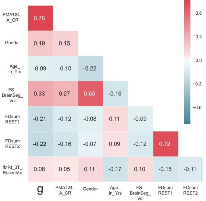
We characterize the relationship between intelligence and each of the confounding variables listed above in our subject sample (Figure 2). Intelligence is correlated with gender (men scored higher in our sample), age (younger scored higher in our sample -- note the limited age range 22-36 y.o.), and brain size (larger brains score higher) [43,44]. There is no
relationship between handedness and intelligence in our sample (r=2x10⁻⁶). Motion, quantified
as the sum of frame-to-frame displacement over the course of a run (and averaged separately for REST1 and REST2) is correlated with intelligence: subjects scoring lower on intelligence moved more during the resting-state. Note that motion in REST1 is highly correlated (r=0.72) with motion in REST2, indicating that motion itself may be a stable trait, and correlated with other traits. While the interpretation of these complex relationships would require further work outside the scope of this study (using partial correlations, and mediation models, to disentangle effects), it is critical to remove shared variance between intelligence and the primary
confounding variables before proceeding further. This ensures that our model is trained
specifically to predict intelligence, rather than confounds that covary with it in our subject sample [115]. However there are several other variables that we do not explicitly account for here, for example the Openness personality trait which we previously found to be correlated with intelligence [65].
Another possible confound, specific to the HCP dataset, is a difference in the image reconstruction algorithm between subjects collected prior to and after April 2013. The
reconstruction version leaves a notable signature on the data that can make a large difference in the final analyses produced [116]. We find a small, but significant correlation with the
intelligence in our sample (indicating that subjects imaged with the old reconstruction version are, on average, less intelligent than the ones imaged with the newer reconstruction version). This confound is, of course, a simple sampling bias artifact with no meaning. Yet, this significant artifactual correlation must be removed, by including the reconstruction factor as a confound variable.
Importantly, the multiple linear regression used for removing the variance shared with confounds is fitted on the training data (in each cross-validation fold during the prediction analysis), and then the fitted weights are applied to remove the effects of confounds in both the training and test data. This is critical to avoid any leakage of information, however negligible, from the test data into the training data.
Authors of the HCP-MegaTrawl have used transformed variables (Age2) and interaction
terms (Gender x Age, Gender x Age2) as further confounds [117]. After accounting for the
confounds described above, we do not find sizeable correlations with these additional terms (all correlations <0.011), and thus we do not use these additional terms in our confound regression.
Figure 2. Correlation of the general intelligence factor scores with PMAT24_A_CR scores, and with potential confounds, in the sample of subjects used for prediction analyses (N=884). All of these variables except for PMAT24_A_CR scores were regressed out of the training set data to obtain an unconfounded measure of g.
Resting-state FC predicts 20% of the variance in
g
across
subjects
We compute a resting-state functional connectivity matrix for each subject from 1 hour of resting-state data (REST12), yielding a very reliable estimate of the stable functional network of each individual -- with 60 minutes of scan time, the test-retest reliability of the FC matrix is above r=.96 [118].
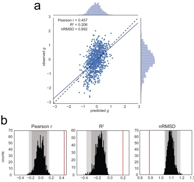
We use a leave-one-family-out cross-validation scheme to train a regularized linear model and predict general intelligence from functional connectivity matrices (features are the 64620 undirected edges), in our sample of 884 subjects. We find a significant correlation between observed and predicted g scores (r=0.457, p1000<0.001, based on 1000 permutations), a coefficient of determination that differs significantly from chance (R2=0.206; p
1000<0.001), and
a normalized root mean square deviation that is significantly lower than its null distribution (nRMSD=0.892;p1000<0.001) (Figure 3).
For comparison, we find that the prediction of PMAT24_A_CR captures less variance (r=0.263,p1000<0.001; R2=0.047, p
1000<0.001; nRMSD=0.977, p1000<0.001). It is likely that the
moderating effect of measurement quality [44] limits prediction performance.
Similarly, using only 30min of resting-state data to derive the functional connectivity matrices has a moderating effect on prediction performance. With 30 minutes of scan time, test-retest reliability of FC matrices falls to about r=.92 [118]. Predicting g using REST1, we find r=0.419, R2=0.170, nRMSD=0.912; using REST2, we find r=0.312, R2=0.067, nRMSD=0.966.
Figure 3. Prediction of the general factor of intelligence g from resting-state functional connectivity, averaging all resting-state runs for each subject (REST12, totaling 1h of fMRI data). a) Observed vs. predicted values of the general factor of intelligence. The
regression line has a slope close to 1, as expected theoretically [98]. The correlation coefficient is r=0.457 (REST1 only, r=0.419; REST2 only, r=0.312). b) Evaluation of prediction
performance according to several statistics and their distributions under the null hypothesis, as simulated through permutation testing (with 1000 surrogate datasets). All fit statistics fall far out of the confidence intervals under the null hypothesis. Left: the correlation between observed and predicted values; Center: the coefficient of determination R2, interpretable as the proportion of
explained variance; Right: the normalized Root Mean Square Deviation nRMSD, which indicates the average difference between observed and predicted scores. Faint gray shade: p<0.05; darker gray shade: p<0.01, permutation tests.
Predictive edges are distributed in FPN, CON, DMN, and VIS
networks
We have demonstrated that a substantial and statistically highly significant amount of variance (about 20%) in general intelligence g across our sample of subjects can be predicted from resting-state functional connectivity. Is there a specific set of edges (connectivity between specific anatomical parcels) in the brain that carry most of the information? The Parieto-Frontal Integration Theory (P-FIT) of intelligence [38] postulates roles for cortical regions in the
prefrontal (BA 6, 9–10, 45–47), parietal (BA 7, 39–40), occipital (BA 18–19), and temporal association cortex (BA 21, 37).
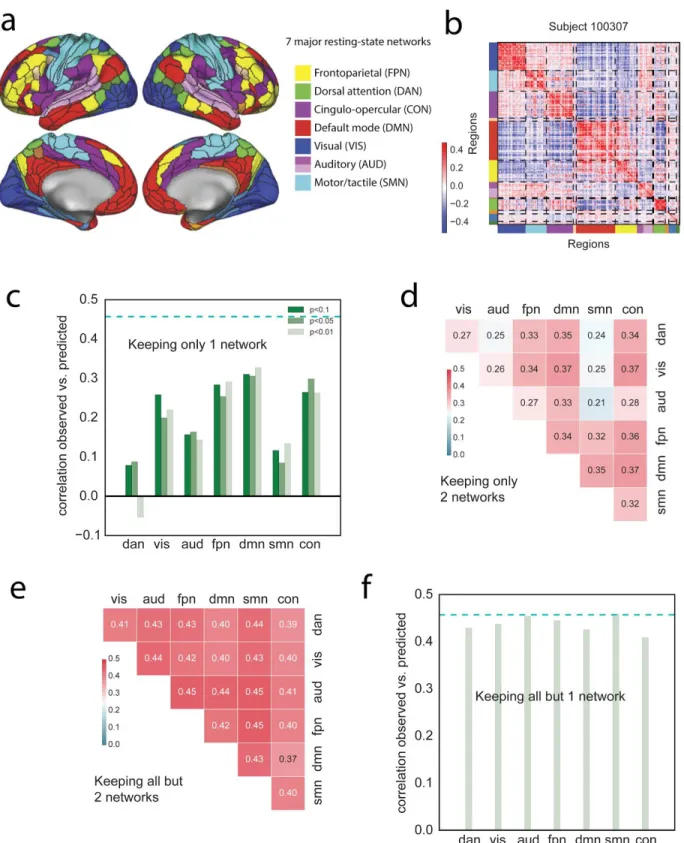
To address this question, we use a descriptive network selection/elimination approach. We focus on the 7 major resting-state networks [119]; Ito and colleagues recently assigned each region of the parcellation used here to these functional networks using the Generalized Louvain method for community detection with resting-state fMRI data [97] (Figure 4a). This network assignment indeed groups regions that have similar connectivity patterns, at the level of single subjects (Figure 4b). First, we ask how well we can predict g keeping edges within only one network (
(
17)
= 7 combinations, Figure 4c ), or within/between two networks ((
27)
= 21combinations, Figure 4d). For all these analyses we carried out exactly the same methods as described above (including the univariate feature selection step), but training and testing on a reduced feature space (corresponding to only those features (edges) under investigation for questions about the specific networks). Prediction performance within a single network, or with two networks, is much impaired compared to performance with the full set of edges (one network, maximum performance r=0.327; two networks, maximum performance r=0.373); however, some networks carry more information than others: the most informative networks are CON, DMN, FPN and VIS, while DAN, AUD and SMN carry very little information. These results are in good agreement with the P-FIT; in particular, in addition to the eponymous frontal and parietal regions which have been reported in other studies already [55,62], we evidence
information in the VIS network as postulated by P-FIT. We next explore how the virtual lesioning of networks affects prediction: we lesion a single network (
(
76)
= 7, Figure 4f) or two networks ((
75)
= 21 , Figure 4e). We find that lesioning one or two networks has a very small effect on the prediction of g (lesion one network, minimum performance r=0.409; lesion two networks, minimum performance r=0.373), indicating there is distributed and redundant information aboutFigure 4. A distributed neural basis for g.a) Assignment of parcels to major resting-state networks, reproduced from Ito et al. [97]. b) Example REST12 functional connectivity matrix ordered by network, for an individual subject (id=100307). c) Prediction performance for REST12 matrices (as Pearson correlation between observed and predicted scores) using only
within network edges, for the 7 main resting-state networks listed in a. DMN, FPN, CON and VIS carry the most information about g. The three shades of green correspond to three univariate thresholds for initial feature selection (we used p<0.01 as in the main analysis; as well as p<0.05 and p<0.1 to make sure that the results were not limited by the inclusion of too few edges). The dashed cyan line shows for comparison the prediction performance for the
whole-brain connectivity matrix (same data as in Figure 3). d) Prediction performance with two networks only (univariate feature selection with p<0.01). e) Prediction performance for REST12 matrices after “lesioning” two networks (univariate feature selection with p<0.01). f) Prediction performance after lesioning one network (univariate feature selection with p<0.01).
Discussion
Deary et al. recently wrote [120]: “the effort to understand the psychobiology of
intelligence has a resemblance with digging the tunnel between England and France: We hope, with workers on both sides having a good sense of direction, that we can meet and marry brain biology and cognitive differences.” The present study is a step in this direction, offering to our knowledge the to-date most robust investigation specifically focused on predicting intelligence from resting-state fMRI data. Here we used factor analysis of the scores on 10 cognitive tasks to derive a bi-factor model of intelligence, including a common g-factor and broad ability factors, which is the standard in the field of intelligence research [28,44]. We used reliable estimates of functional connectivity in a large sample of subjects, from one hour of high-quality resting-state fMRI data per subject. We used the best available inter-subject alignment algorithm (MSM-All), a stringent control for confounding variables, and out-of-sample prediction. With these
state-of-the-art methods on both ends of the tunnel, we demonstrated a strong relationship between general intelligence g and resting-state functional connectivity (at least as strong as the well established relationship of intelligence with brain size [43,44]). We further established that predictive network edges were fairly distributed through the brain, though they mostly fell within 4 of the 7 major resting-state networks: the fronto-parietal network, the default mode network, the control network, and the visual network. These findings are in general agreement with the parieto-frontal integration theory (P-FIT) of intelligence. They considerably extend a previous report [62] which had hinted at a relationship between resting-state functional connectivity and intelligence using a much smaller subject sample (N=117), no account of potential confounding variables, a cross-validation scheme that did not respect family structure, a less functionally accurate inter-subject alignment, and a lower quality measure of intelligence.
We indeed found evidence that measurement quality, both on the behavioral and on the neural side, moderated the effect size of the relationship between brain and behavior [44]. We achieved better prediction performance using g rather than the number of correct responses on the PMAT24_A test; and we achieved better performance using REST12 matrices (1h of data per subject) rather than REST1 or REST2 matrices (30min of data per subject). Though this is of course expected statistically -- the noise ceiling gets lower as noise increases for the two variables that are correlated -- this is an important observation for future explorations in other datasets. In many aspects the neural and behavioral data in the HCP are of higher quality than
most other large-scale neuroimaging projects; conducting similar analyses in other datasets may yield smaller effect sizes solely because of lower data quality and, just as importantly, quantity.
The general factor of intelligence g that we derived from 10 cognitive task scores is as reliable as it can be in this dataset, and would be unlikely to improve substantially even if additional measures were available. An interesting question for future studies will be to look at the predictability of the subscales: crystallized ability, processing speed, visuospatial reasoning, and memory. Addition of tasks in each of these subdomains would increase the reliability of these specific ability factors, and allow for a more precise exploration of their neural bases. This would require a much longer assessment and many more ability tests. Rather than build an entirely new dataset from scratch, the possibility of testing all HCP subjects again on a lengthier, diverse cognitive ability battery should be considered [121].
Another factor that can moderate the relationship between variables is range restriction of variables [122]. Here, there is some concern that the range of intelligence scores in the HCP subject sample may be restricted to the higher end of the distribution. While published
normative data is currently unavailable for the Penn matrix reasoning test and other Penn CNB tests in the age range of our subjects, the NIH toolbox tests provide age-normed scores. Inspection of these scores indicates that the HCP subject sample is indeed biased towards higher scores (in particular for crystallized abilities; see Supplementary Figure 3). This
sampling bias is a well-known, systemic issue in experimental psychology [123], and one that is difficult to avoid despite efforts to recruit from the entire population. A natural question to ask is whether the neural bases of mental retardation, and of genius at the other end of the spectrum, lie in the same continuum as what we describe in this study. Future studies in samples with a larger range of intelligence should explore this important question.
Though we qualified our approach as state-of-the-art on the behavioral side, intelligence researchers would likely object that deriving factor scores is a thing of the past, and that
analyses should be conducted in latent space (in part because of factor indeterminacy). This objection can mostly be ignored in our situation, where we only looked at the general factor g, given that it can be so precisely estimated in our dataset. However to study specific factors, it would be advisable to overhaul our predictive analysis so it can be performed in latent space, within a structural equation model. Others have explored such a framework in the study of brain-behavior relationships [41].
We were very careful to regress out several potential confounds [115], such as brain size, gender and age, before performing predictions. While this gives us some comfort that the results reported here are indeed specific to general intelligence, the confound regression approach could certainly be improved further. There are two main concerns: one the one hand, we may be throwing out relevant variance and injecting noise into the g scores by bluntly regressing out confounding variables -- a more careful cleanup should be attempted, for
example using a well-specified structural equation model [124]. However, the approach we took is superior to ignoring the issue of potential confounds altogether, which is likely to inflate
predictability and compromise interpretation. On the other hand, the list of confounding variables that we considered was not exhaustive: for example, we did not regress out variance in the Openness factor of personality, which we have previously found to be correlated with
intelligence [65], and there are certain to be other confounds that were not measured at all. Furthermore, it is very likely that regressing out the mean framewise displacement does not properly account for non-linear effects of motion. Cleaning resting-state fMRI data of the effects of motion remains a very intense topic of research for studies of brain-behavior relationships [83,85,125]. While we are confident that our current results are not solely explained by motion in the scanner, a full quantification of this issue remains warranted.
It is worth mentioning a related, entirely data-driven study that was recently conducted by Smith and colleagues on an earlier release of the same HCP dataset (N=461) [126]. Using canonical correlation analysis, the authors demonstrated that a network of brain regions that closely resembled the default mode network was highly related to a linear combination of behavioral scores that they label a “positive-negative mode of population covariation”. In essence, this combination is a neurally derived general factor, encompassing cognitive and other behavioral tasks. Our study is in good agreement with these results, as we found high predictability of general intelligence g from connections within the default mode network.
Where do we go from here? As we know that task functional MRI [38,56] and structural MRI data (brain size [43], as well as morphometric features [82]) also hold information that is predictive of cognitive ability, a natural question is whether combining functional and structural data will allow us to account for more variance in the general intelligence factor g. The more variance we can account for, the more trustworthy and thus interpretable our models become, and we can hope to further refine our understanding of the neural bases of general intelligence.
Of course, mere prediction does not yet illuminate mechanisms, and we would ultimately wish to have a much more detailed causal model that explains how genetic factors, brain
structure, brain function, and individual differences in variables such as g and personality relate to real-life outcomes. Given that g is already known to predict outcomes such as lifespan and salary, a structural model incorporating all of these variables should provide us with the most comprehensive understanding of the mechanisms, and the most effective information for targeted interventions.
Finally, we would like to situate this paper in the broader context of this special issue. Intelligence can be quantified across species and is highly heritable. Are similar brain networks the most predictive of variability in intelligence across mammals? Are there measures of heritability or brain structure, as compared to brain function, that might be better predictors in some species than others? It would be intriguing to find that humans share with other species a core set of genetically specified constraints on intelligence, but that humans are unique in the extent to which education and learning can modify intelligence through the incorporation of additional variability in brain function.
Author contributions
J. Dubois and P. Galdi developed the overall general analysis framework and conducted some of the initial analyses for the paper. J. Dubois conducted all final analyses and produced all figures. L. Paul helped with literature search, analysis of behavioral data, and interpretation of the results. J. Dubois and R. Adolphs wrote the initial manuscript and all authors contributed
to the final manuscript. All authors contributed to planning and discussion on this project. The authors declare no conflict of interest.
Acknowledgments
This work was supported by NIMH grant 2P50MH094258 (PI: RA), the Chen
Neuroscience Institute, the Carver Mead Seed Fund, and a NARSAD Young Investigator Grant from the Brain and Behavior Research Foundation (PI: JD). We thank Stuart Ritchie, Gilles Gignac, William Revelle, and Ruben Gur for invaluable advice on the behavioral side of the analyses -- though the final analytical choices rest solely with the authors.
Data Sharing
The Young Adult HCP dataset is publicly available at
https://www.humanconnectome.org/study/hcp-young-adult. Analysis scripts are available in the following public repository: https://github.com/adolphslab/HCP_MRI-behavior.
References
1. Gottfredson LS. 1997 Mainstream science on intelligence: An editorial with 52 signatories, history, and bibliography.
2. Gottfredson LS. 1997 Why g matters: The complexity of everyday life. Intelligence24, 79–132.
3. Jensen AR. 1981 Straight talk about mental tests. The Free Press.
4. Burkart JM, Schubiger MN, van Schaik CP. 2016 The evolution of general intelligence.
Behav. Brain Sci. , 1–65.
5. Plomin R, Deary IJ. 2015 Genetics and intelligence differences: five special findings. Mol.
Psychiatry20, 98–108.
6. Kuncel NR, Hezlett SA. 2010 Fact and Fiction in Cognitive Ability Testing for Admissions and Hiring Decisions. Curr. Dir. Psychol. Sci.19, 339–345.
7. Strenze T. 2007 Intelligence and socioeconomic success: A meta-analytic review of longitudinal research. Intelligence35, 401–426.
8. Deary IJ, Taylor MD, Hart CL, Wilson V, Smith GD, Blane D, Starr JM. 2005
Intergenerational social mobility and mid-life status attainment: Influences of childhood intelligence, childhood social factors, and education. Intelligence33, 455–472.