Attractor Metafeatures and Their Application in Biomolecular Data Analysis

(1)

Attractor Metafeatures and Their Application in Biomolecular Data Analysis

Tai-Hsien Ou Yang

Submitted in partial fulfillment of the

requirements for the degree of

Doctor of Philosophy

in the Graduate School of Arts and Sciences

COLUMBIA UNIVERSITY

2018

(2)

(3)

ABSTRACT

Attractor Metafeatures and Their Application in

Biomolecular Data Analysis

Tai-Hsien Ou Yang

This dissertation proposes a family of algorithms for deriving signatures of mutually

associated features, to which we refer as attractor metafeatures, or simply attractors. Specifically, we present multi-cancer attractor derivation algorithms, identifying correlated features in

signatures from multiple biological data sets in one analysis, as well as the groups of samples or cells that exclusively express these signatures. Our results demonstrate that these signatures can be used, in proper combinations, as biomarkers that predict a patient’s survival rate, based on the transcriptome of the tumor sample. They can also be used as features to analyze the composition of the tumor.

Through analyzing large data sets of 18 cancer types and three high-throughput platforms from The Cancer Genome Atlas (TCGA) PanCanAtlas Project and multiple single-cell RNA-seq data sets, we identified novel cancer attractor signatures and elucidated the identity of the cells that express these signatures. Using these signatures, we developed a prognostic biomarker for breast cancer called the Breast Cancer Attractor Metagenes (BCAM) biomarker as well as a software platform to analyze the tumor sample, called Analysis of the Single-Cell Omics for Tumor (ASCOT).

(4)

List of Figures

Figure 2.1 (A) Strength and (B) number of attractors against exponent 𝜶 for the

consensus-attractor derivation method in TCGA bulk data sets. ...30

Figure 2.2 (A) Strength and (B) number of attractors against exponent 𝜶 for the consensus-attractor derivation method in scRNA-seq data sets. ...30

Figure 3.1 Scatter plots of(A) CD53, SASH3, IL10RA in 18 TCGA data sets, (B) Leukocyte, M+, M- attractor metafeatures in 17 TCGA data sets ...45

Figure 3.2 Scatter plots of (A) the T-cell signature and (B) the B-cell signature against the mitosis signature. ...57

Figure 3.3 Top hits of the MSigDB gene-set enrichment analysis against the top genes of the stem-like signature. ...59

Figure 3.4 Scatter plots of the stem-like signature against the fibroblast signature (A) in the melanoma data set and (B) in the breast cancer data set. ...60

Figure 3.5 Boxplots of the expression levels of the stem-like signature by type of cells in (A) the melanoma data set and in (B) the breast cancer data set. ...60

Figure 4.1 Screenshot of the feature-selector facility. ...66

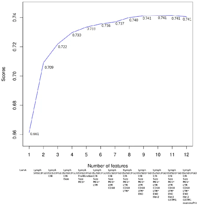
Figure 4.2 Scatter plot of the YAP1 and the SMAD6 proteins in the AML patients. ...70

Figure 4.3 Scores of the optimal combinations of different numbers of the features. ...74

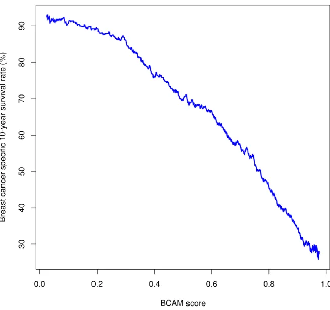
Figure 4.4 Estimated breast cancer-specific ten-year survival rate as a function of the BCAM score. ...76

Figure 4.5 Kaplan–Meier plots of (A) FGD3-SUSD3 and (B) ESR1 in breast cancer data sets. ..78

Figure 4.6 Frequency distributions of BCAM scores for subgroups of ER-negative breast cancer cases. ...82

Figure 5.1 Relationships of the exponent for metacell discovery and the number of discovered metacells in the annotated scRNA-seq data set GSE36552...90

Figure 5.2 t-SNE plot of the classification result of the samples from (A) melanoma patient CY79 and (B) melanoma patient CY84. ...93

Figure 5.3 Boxplots of the stem-like signatures by the type of cells in (A) the cells from patient CY79 and (B) the cells from patient CY84 of the melanoma data set. ...94

(6)

List of Tables

Table 3.1 List of the TCGA Data Sets Analyzed in This Study ...39

Table 3.2 List of Consensus-Attractor Signatures in the TCGA PanCanAtlas Data Sets ...41

Table 3.3 List of the scRNA-seq Data Sets Used in the Derivation of the Single-Cell Consensus Attractors ...54

Table 3.4 List of the Consensus Attractors in the scRNA-seq Data Sets ...54

Table 4.1 The Breast Cancer Data Sets Analyzed in this Study ...63

Table 4.2 The BCAM Model ...67

Table 4.3 List of the Concordance Index Scores of Each Prognostic Assay on the Breast Cancer Data Sets and the Subgroups of Cases ...79

Table 5.1 List of the Annotated scRNA-seq Data Sets Analyzed in this Study ...88

(7)

Acknowledgements

I thank my advisor, Prof. Dimitris Anastassiou, who was not only a wonderful mentor but also a great working partner. I wish to thank Wei-Yi Cheng and Kaiyi Zhu for their help and feedback on this work. I am also grateful to the collaborative partners who contributed to this work; in particular, Abdulkadir Elmas and Prof. Xiaodong Wang. I thank Wei-Yi Cheng, Tsai-Wei Chiu, and Kaiyi Zhu for their company during my pursuit of the degree. Finally, I would like to thank my parents, Hui-Ming Ou Yang and Ya-Jung Lee, and my sister Tai-Ya Ou Yang, for their continuing support and encouragement along the way.

(8)

(9)

Chapter 1 Introduction

1.1 Background

Cancer remains one of the major causes of death in the world [1] but lacks universally effective diagnostic and therapeutic regimens. Cancer consists of a group of diseases that may affect any body part, characterized by the abnormal growth of a group of cells that may invade adjacent tissues and metastasize to other organs. Despite the progress in the development of therapeutic regimens and diagnostic tools in the last two decades, knowledge of the details of the biological mechanisms in cancer to aid in developing diagnostic tools and therapeutic agents is still limited.

The lack of knowledge about biological mechanisms is partially due to the diversity of this family of diseases. Knowledge of how the cause of the disease aligns with changes in the genome [2] would make it possible to shed light on the biological mechanisms by analyzing alterations in the genome of a tumor cell. The characteristics of the family of diseases may differ from one organ of origin to another, from one patient to another, even in the same tissue, because of its evolutionary nature [3-9]. Many cell subpopulations and underlying biological process are involved in the interactional process of the formation of cancer, or oncogenesis, and the

progression of cancer [10, 11]. Such biological processes involve numerous molecular components.

Such complexity not only obstructs the development of precise tools for diagnosis and the discovery of the “universal cure” to the disease, but also hinders the reconstruction of the biological mechanism, because conventional research techniques of molecular cell biology are only suited for study of one component of the cell at a time, using a small batch of samples.

(10)

Furthermore, the assessment of the efficacy of a new regimen relies on extensive clinical studies and a trial-and-error methodology.

Recent breakthroughs of high-throughput cell biology technologies enable scientists to capture the molecular characteristics of components across the whole genome and many

pathologic tissues in tractable time and budget. This opportunity provides the ability to study the disease by simultaneously analyzing the association of all such molecular characteristics with clinical phenotypes and the association of all molecular components with each other, using a set of samples that is large enough to ensure sufficient statistical power for analysis. With such holistic information about the disease, biologists may be able to model the heterogeneity of the disease and reconstruct the underlying biological mechanisms, eventually developing an effective diagnosis and treatment regimen with high precision.

High-Throughput Cell Biology Technologies

In a biological system, the “central dogma” dictates transfer of genetic information from one type of biomolecule containing a biological sequence to another type of biomolecule [12-14]. Genetic information is stored in sequences of deoxyribonucleic acid (DNA), which are “transcribed” into the corresponding sequences of ribonucleic acid (RNA). The sequences of some RNAs are “translated” into the sequences of amino acids.

In the 1970s, researchers proposed many commercialized technologies for qualitative and quantitative characterization of specific biological sequences, some of which remain in wide use in cell-biology research. For qualitative methods, the southern blot [15] and the northern blot [16] detect specific DNA and RNA sequences in a biological sample. Because a single-stranded nucleic acid sequence binds to its complementary counterpart, these methods detect the presence of a target sequence using a labeled sequence that is complementary to the target, called the

(11)

hybridization probe. Later, researchers proposed quantitative reverse transcription PCR

(RT-qPCR) as a more sensitive alternative to the northern blot [17], suggesting the western blot [18] to detect specific protein sequences, exploiting the binding specificity of the antibody to the corresponding proteins. For qualitative analysis, Sanger et al. introduced the sequencing method, or the chain-termination method, to determine the DNA sequence [19]. The method incorporates a special type of labeled nucleotides that can temporarily cease the synthesis of a DNA sequence from a template, allowing observations of the order of the nucleotides of the sequence.

The drawback of these techniques is that they are suited only for interrogating one or a few targets in one experiment. Due to the large number of molecular components involved in the biological process, modeling the pathogenic process of a complicated disease such as cancer was unattainable at the time.

Researchers developed the multiplex automated versions of these methods in the 1990s and the concept of interrogating a large number of targets in one experiment became practical. By fixing various DNA hybridization probes onto many microscopic spots on a plane, the

microarrays massively quantified DNA [20] and later the RNA sequences by incorporating reverse transcription. Using bisulfite conversion, which is a procedure that converts the unmethylated cytosine residues in the DNA sequence to uracil, the microarrays can quantify DNA methylation levels across the entire genome [21]; by incorporating the chromatin immunoprecipitation (ChIP) techniques, scientists can use the microarrays to study the

interactions of the DNA sequence and proteins [22]. Thus, quantifying all DNA, the “genome,”

all RNA, or the transcriptome, and the DNA methylation levels of the genome, the methylome,

in a sample became practical for biomedical research, and the field of study using these objects is

(12)

The massive automation of Sanger sequencing was the cornerstone of the effort to map the human genome [23]. Modern high-throughput sequencing systems identify, for each person, the exact sequence of the whole human genome and its single nucleotide polymorphisms (SNPs) and copy number alterations (CNAs) by comparison with a reference genome. High-throughput sequencing methods allow the incorporation of techniques that transform information into DNA sequences. The method can be extended to quantify all RNAs by incorporating reverse

transcription, called RNA-seq [24], to profile DNA methylation levels by incorporating bisulfite conversion, called bisulfite sequencing [25], or to investigate DNA-protein interactions using ChIP techniques, called ChIP-seq [26]. Recently, high-throughput sequencing methods to

analyze the sequences in a single cell, such as scDNA-seq [3, 6, 27, 28], scRNA-seq [29-31], and scBS-seq [32], became available because the technical difficulty of sequencing using the low input of DNA and RNA was overcome. Biomolecular techniques used in single-cell sequencing methods were developed specifically for the particular circumstances required to study single cells with an extremely limited amount of input. Therefore, the properties of such data are different from those of their “bulk” counterparts.

For the study of many proteins in a sample, biologists proposed several methods such as the reverse-phase protein assay (RPPA) [33] and mass spectrometry (MS)-based methods [34, 35]. Because the availability of these high-throughput technologies has encouraged efforts on profiling and studying new biological samples of all species and health conditions, massive amounts of data have been generated. To help archive and share these data, scientists set up several database repositories for public access. For the omics data sets of all types of biological samples, such repositories are the Gene Expression Omnibus (GEO) [36], the Sequence Read Archive (SRA) [37], the database of Genotypes and Phenotypes (dbGaP) of the National Center

(13)

for Biotechnology Information [38], and ArrayExpress of the European Bioinformatics Institute of the European Molecular Biology Laboratory (EMBL-EBI) [39]. For the omics data sets of human cancer samples, The Cancer Genome Atlas (TCGA) [40-48], The International Cancer Genome Consortium (ICGC) [49], and the American Association of Cancer Research (AACR) Project Genomics, Evidence, Neoplasia, Information, Exchange (GENIE) [50] are projects dedicated to share data for all types of cancer.

The data sets generated using high-throughput technologies typically can be presented as a matrix, in which the rows and the columns conventionally represent the molecular components or the “features,” such as genes, and the samples (or cells) profiled in the study, or the

“observations,” respectively. The value of each element in the matrix represents the quantity or the presence of a molecular component in the particular sample and the distribution of values reflects the biological property of the samples. Thus, one can formulate the analysis of biological data into a machine-learning framework. In the context of cancer research, using unsupervised machine-learning techniques one can discover the features and samples that share similar

patterns in a data set, such as the functional modules of the biological components or subtypes of the disease. If the data set is annotated with the clinical phenotypes of patients, the association of biological components with the phenotypes can be clarified and modeled using supervised machine-learning techniques [51].

Distinct challenges accompany the analysis of these emerging large data sets, such as excessive computational complexity. Furthermore, the number of features is typically much larger than the number of samples, which affects the reliability of conventional statistical methods. The values in the matrix are noisy, due to the stochastic data-capturing nature of the technologies, and can be affected by variations, such as batch effects. Each type of data also has

(14)

its own distinct property. For example, the matrix of an RNA-seq data set is typically sparse and suffers from overdispersion, i.e., variance larger than expected [52]. These concerns need to be addressed during the analysis and to be considered during the development of new methods for high-throughput data analysis.

1.2 Prior Work on Cancer Signature Identification

Cancerous cells display several molecular traits that are different from those normal cells of the same type. Certain molecular measurements aligned with the pathogenic states of cancer, such as the level of a specific protein in blood and the activity of a set of genes in tumor samples. These measurements can be developed as indicators of the pathogenic process and predictors of the benefit of therapeutic treatments, called “biomarkers.” A type of cancer may be stratified into multiple subgroups based on the characteristics of the cells. These subgroups of types are called

subtypes, and may influence the response to a treatment and the prognosis of the patient. The

validity of a biomarker may be specific to a particular subtype of cancer.

Clinical practitioners have introduced biomarkers and subtyping systems to help evaluate the benefit of treatment for a patient. For example, for patients in the early stage of certain subtypes of breast cancer, some available and commercialized genomic tests are the OncotypeDX test [6], Prosigna assay (PAM50) [7], and the MammaPrint test [8].

Despite the diversity of pathological manifestations in various types and subtypes and the markers that indicate the pathogenic states for each of them, Douglas Hanahan and Robert Weinberg proposed that cancer has general unifying capabilities, or “cancer hallmarks” [6]. It is reasonable to hypothesize that: 1) some traits of the molecular components are represented by particular patterns detectable in biomolecular data sets containing measurements derived from

(15)

cancer samples; and 2) the molecular components with similar patterns of the traits are involved in the same biological process, which may also relate to the pathogenic process.

Therefore, a discovery path for such universal traits and toward the development of the corresponding multi-cancer biomarkers for diagnosis, prognosis, and treatment-response prediction can build on computational analysis of the large high-throughput data sets coming from biopsies of numerous patients and from many different cancer types.

Clustering Analysis

Clustering analysis is a family of unsupervised learning methods that organize the unlabeled items in a data set into multiple groups by a similarity metric. Among the clustering methods, hierarchical clustering and centroid-based clustering methods have been in wide use in the research on cancer signatures.

Hierarchical clustering algorithms may assign the items into clusters by successively

partitioning or merging them, according to a similarity measure, often in the development of heat maps, which are visualization tools for a matrix of biological data, with the potential to identify correlated features as biological signatures and groups of samples as subtypes. For single-cell data sets, researchers use such algorithms to identify the populations of cells [9, 53, 54]. The signatures found using hierarchical clustering analysis facilitated the development of

commercialized cancer biomarkers, such as MammaPrint [55]. Hierarchical clustering is an intuitive and deterministic method used in helping visualize high-throughput data for presenting the modules of correlated molecular components as signatures and similar samples as subtypes.

Centroid-based clustering methods assume a centroid of each cluster in the data and partition the items into these clusters by their similarity with centroids, and refine partitioning in an

(16)

that partitions the items into k clusters. In an iterative process, the algorithm assigns the items to the cluster with the nearest mean and updates the centroid of each cluster until it satisfies a

stopping criterion. A closely related method is called k-medoids, which uses data points instead

of the mean of the points as the centers and minimizes the sum of distances of the data points to their medoids by swapping a medoid with a non-medoid at each iteration. Researchers used a realization of the method, PAM, to identify a set of fifty genes that classify breast cancer tumors into four subtypes, called PAM50. Parker et al. used the gene set in PAM50 in a commercialized biomarker product to evaluate the risk of distant recurrence of breast cancer patients [57].

Researchers not only apply clustering analysis to gene expression data, but also to mutation data [58, 59], copy number variation (CNV) data [60], and DNA methylation data [61]. To address the properties of the emerging single-cell data sets, scientists have proposed multiple novel approaches, introduced in Chapter 5.

An obvious limitation of centroid-based methods is that they require a predefined set of initial points. A solution is to randomly select the initial points and repeat the algorithm multiple times, leading to a nondeterministic result. To cluster the items without selecting initial points, researchers proposed a variation of density-based clustering methods, called DBSCAN. The method clusters the items by their density in the space. It has been used to cluster the cell populations of the melanoma scRNA-seq data set [62]. A drawback of the method is that it is difficult to select an appropriate parameter and assumes similar densities around the groups in a data set, which may not always be the case in the biological data.

The possibilities of identifying coexpression signatures across multiple data sets was explored with clustering methods. A method called the cluster-of-clusters assignment (COCA) was applied to the data of six omics platforms of 3,527 samples from 12 cancer types of the

(17)

TCGA data sets [59] identifying a set of cross-tumor-type molecular signatures and classification of subtypes. To cluster the features and the samples across data sets, the COCA algorithm

incorporates the information of platform-specific clusters as a set of binary vectors so the method re-clusters them based on these vectors. The documented cancer signatures were then introduced to analyze the characteristics of subtypes. Although the method incorporated normalization steps, it does not address the distinctiveness of the tissues of origin. Therefore, the subtypes it found were approximately consistent with their tissues of origin. The result suggested that some known signatures can be found in the samples from different tissues of origin, but the method was not designed to identify novel universal signatures.

As a closely related effort, a clustering method, called CoINcIDE , clusters cancer samples across multiple data sets [63]. It evaluates the similarities of each pair of clusters found in each data set and assigns weighted edges between the pairs that are close; thus, it finds “metaclusters” as subtypes. As a different approach to analyze multiple data sets, researchers have proposed methods that model each data set using a mixture model and integrate the data sets using the other model for integrative clustering [64, 65]. Because these methods assume structural

similarity in the data sets [66], they are not applicable to data sets with dramatic differences, such as data sets from different types of cancer.

A different approach is to capture the characteristics of the data sets using mathematical models to perform cross-data-set clustering. For example, iCluster [64] uses a joint variable model to model multiple data sets and to perform integrative clustering across multiple data sets and data types. Multiple Dataset Integration (MDI) employs the Dirichlet-multinomial allocation (DMA) mixture model to model multiple data sets [65].

(18)

Dimensionality Reduction

Principal-component analysis (PCA) has been the most popular method to reduce the number of dimensions, visualizing the similarities of genes or samples in a data set, making the cancer signatures and subtypes observable. PCA projects values through linear transformation to the orthogonal planes that maximize the variance of the projection, “explaining” variations in the data [67]. A related method is independent-component analysis (ICA), which poses component analysis into a task of matrix factorization in which the data matrix is the product of a mixing matrix and a set of hidden variables that can be used to identify cancer signatures [68].

The t distributed stochastic-neighbor-embedding (t-SNE) method has been gaining popularity

to address problems of dimensionality reduction. t-SNE minimizes divergence between: 1) the original data in which the similarity of a pair of points is defined as a distribution in high-dimensional space; and 2) a low-high-dimensional space in which the similarity is defined as, for example, a t distribution [69]. t-SNE does not assume linearity in the relationship of data points, so it typically outperforms PCA on biological data. In contrast to PCA, t-SNE is not a

deterministic method and its computational complexity is far larger than that of PCA. Because it does not produce a transformation from the original data space to the projected plane, it cannot be easily used to process the incoming data. For the analysis of single-cell transcriptome data [62], t-SNE is applied on PCA-transformed data so the computational complexity is tractable, while including as many dimensions as possible in the analysis.

A closely related family of methods identifying sets of the similar genes and samples is matrix factorization, performed by decomposing a matrix into two or more matrices.

Nonnegative matrix factorization (NMF) is one of its most widely used variations. It decomposes a nonnegative data matrix into two nonnegative matrices that represent signatures as the

(19)

weighted sum of genes and the levels of signatures in the samples. Matric factorization is suitable for analyzing RNA-seq data, because the measurement is the count of molecules. NMF has been used in many studies identifying cancer signatures [70]. The drawback of NMF is that it is ill-posed, allowing nonunique solutions from the factorization. Furthermore, the values in the decomposed matrices do not necessarily represent the significance of the signature, so the decomposition cannot be immediately interpreted as cancer signatures [71].

Attractor Signatures

Modules of highly correlated genes, defining a co-expression signature, are assumed to represent a particular biological process. One of the most popular methods is weighted gene co-expression network analysis (WGCNA), which constructs the set of the correlated genes in a data set by connecting the genes using the weights based on a similarity function [72].

Researchers also have proposed several regulatory network reconstruction methods that leverage mutual information (MI) or the tree-based method to capture nonlinear interactions between genes [73-75]. Since single-cell sequencing technology has become available, researchers also have introduced methods that analyze biological network, using single-cell gene-expression data [76].

The co-expression signature identification methods mentioned above assume a set of mathematical constraints, such as mutual exclusivity or orthogonality, and ideal biological premises on input data. However, in actual biological systems, such assumptions may not represent reality, for example, matrix factorization methods may not accurately capture

co-expression events with biological significances. Thus, an algorithm without any constraints should be devised to identify the signatures as surrogates of the biological processes.

(20)

We proposed an unsupervised iterative algorithm that identifies signatures called “attractor metagenes” (more generally “attractor metafeatures”) [77] without using such assumptions on the input data. To understand such an algorithm, we can start with a hypothetical case. For example, we found a cluster of correlated genes in a gene expression data set. Thus, we would like to scrutinize them as a coexpression event and try to “sharpen” the coexpression to find out the gene at the “heart” (core) of the underlying co-expression.

Given that the phenotype is absent, we can repeatedly apply an unsupervised approach, described as follows: We can define a metagene from the average expression levels of all genes within the cluster of correlated genes, and rank all the individual genes of the data set in terms of their association with that metagene. Then we substitute an equal number of the top-ranked genes for genes from the cluster of correlated genes. Several of the original genes may stay at the top of the list and the rest will be replaced. This process “attracts” some other genes that are more strongly correlated with the cluster.

We can then define a new metagene by the average expression levels of the genes in the new cluster of correlated genes. Then we rank all the genes again in terms of their association with that new metagene, and so on. It is intuitive to expect that this iterative process will eventually converge to a cluster of correlated genes that contains precisely the genes that are most

associated with the metagene of this cluster. We can think of this particular cluster defined by the convergence of this iterative process as an “attractor.”

The above description demonstrates a simplified realization of the attractor derivation

method. Rather than the average of a particular number of gene expression values from a cluster, we define an attractor metagene as the weighted average of all genes where each individual gene has a nonnegative weight, i.e. the attractor derivation algorithm iterates a process that computes

(21)

the associations of a vector with all the features in the matrix, and uses a function of these associations as weights to update the vector as a weighted average of all the features of the matrix, called the “metafeature.” After a sufficient number of iterations, the process converges to a precise “attractor metafeature” to which we simply refer to as an “attractor.” A ranked set of genes specifies each attractor. Their “score,” which measures the strength of their membership in the underlying coexpression, ranks the genes. Therefore, the top-ranked genes of an attractor point to the core (“heart”) of coexpression in the corresponding signature, which is different from classifying features into mutually exclusive groups. This method finds multiple attractors that can be mapped to biomolecular events in a high-throughput data set. In multiple cancer data sets, from many different cancer types the method identified a set of attractors that are nearly identical in composition [77]. Using the data sets of the TCGA Pan-Cancer Project and the attractor method, we identified 18 attractors in very similar composition of the top-ranked features [78].

Many of our attractor metagenes were associated with clinical phenotypes, consistent with the hypothesis that they can be used as cancer signatures. For gene-expression-based attractors, we identified the mitotic chromosomal instability attractor (CIN) associated with the

proliferation of tumor, which is many caused by chromosomal instability in the tumor cells; the mesenchymal attractor (MES) indicating stromal infiltration and mesenchymal transition, associated with invasiveness; the leukocyte-related attractor (LYM), representing immune infiltration; and the endothelial attractor (END) representing endothelial cells in the sample. For the DNA-methylation-based attractors, we found the negatively associated M+ and M- attractors, highly correlated with LYM, consisting of sites over- and under-methylated in the infiltrating immune cells [78].

(22)

The attractor metagenes have been proven to be quantitative surrogates that measure multiple clinical characteristics of cancer, incorporated as features of the winning model for breast cancer survival which was developed by us. It outperformed all other models in the Sage

Bionetworks/DREAM Breast Cancer Prognosis Challenge [79, 80] aimed to evaluate the accuracy of computational models to predict breast cancer patients’ survival time using clinical information, a gene-expression profile, and a copy-number profile.

Given the knowledge of the existence of cancer attractors, we have interest in identifying universal multi-cancer attractor signatures from data sets consisting of multiple cancer types. However, the tissue of origin of tumors also affects gene-expression profiles. Simply

normalizing and concatenating multiple data sets into one large matrix, the pattern identifying algorithms may identify co-expression patterns that are irrelevant to the disease. We present a novel “consensus” attractor derivation algorithm that identifies attractors that represents the same co-expression event in multiple data sets without normalizing and concatenating the data sets in one instance.

1.3 Contributions of the Thesis

We present the development of several attractor derivation methods as powerful tools for identifying signatures with biological significance at the bulk and the single-cell level from different cancer types and data sets including the “consensus” version. With the understanding of the biological significance of the attractor signatures and the experience in the prognostic model development challenges, we developed predictive models for cancer using combinations of the attractor signatures, which demonstrate their clinical significance. Because we discovered that several attractors from single-cell data sets represent specific cell subpopulations, thus can serve

(23)

as the features for analyzing the heterogeneity of a sample, we developed a software platform for analyzing the cell populations using the single cell RNA-seq data.

In this study, we refined the attractor algorithm that we had previously co-developed, which were contributed to and analyzed in the collaborative efforts on The Cancer Genome Atlas Pan-Cancer analysis project [47, 59], and produced a method that systematically identifies attractor signatures across multiple data sets, robust to the bias formed by data-set-specific effects. One novelty of this consensus attractor algorithm is that it is designed to point accurately to few genes that are at the heart of the underlying biological mechanism, while filtering out tissue-specific signals. This method provides an opportunity for us to understand the biology and target potential driver genes, regardless of cancer types. The resulting multicancer signature is called the “consensus attractor.” In a collaborative project, we also proposed a genome-wide method to identify cotransmitted genomic variants, based on the attractor paradigm, called the “attractor metaSNP” [81]. We describe these methods in Chapter 2.

We identified multiple consensus-attractor signatures using the TCGA PanCanAtlas Data Freeze 1.3.1 data sets and statistically confirmed their existence in cancer-type-specific data sets. Other novel aspects of our work include the development of a method to analyze methylation data using 450K array probes, a new version of genomically colocalized attractors identifying amplicons, as well as other CNVs and locally coregulated attractors, pointing to the top-ranked genes in each case. In addition to the multicancer signatures previously identified in general form [77, 82], we also identified the corresponding biological processes and analyzed their clinical significance, such as the prognostic values of attractors discovered in this study. The immune-related consensus-attractor signatures were included in analysis of the TCGA PanCanAtlas

(24)

single-cell RNA-seq data sets, we discovered multiple novel attractors that represent specific tumor subclones and nontumor cells in the microenvironment. We present the results and discoveries in Chapter 3.

We distilled a linear model that predicts the prognosis of a breast cancer patient from a large breast cancer data set using a cross-validation-based feature selection and regression model-fitting approach, presented in Chapter 4. The model consists of the CIN, MES, and

LYM-attractor metagenes and the FGD3-SUSD3 metagene (which we had discovered as the most

protective feature during the challenge), dubbed the Breast Cancer Attractor Metagenes (BCAM) biomarker, validated using multiple independent breast cancer data sets, proven to be more accurate than other methods. Using these methodologies, we also identified a protein attractor signature associated with the response to therapy in the acute myeloid leukemia patients [84].

The attractors found using single-cell data may not only serve as markers for cell-type identification, but also clarify several mechanisms of tumor pathogenesis. Based on this, we developed a platform (“ASCOT”) to identify single-cell attractors and cell populations that can be used to process a new single-cell data set. In Chapter 5, we describe the derivation of the single-cell transcriptome attractor metafeatures and the development of the cell-classification platform to analyze the tumor and its microenvironment.

(25)

Chapter 2 Derivation of the Attractor Metafeatures

2.1 Introduction

The attractor-derivation algorithm is an unsupervised, iterative transformation process, used to identify attractor metafeatures such as the coexpression signatures in individual

high-throughput cancer data sets. Such signatures, in proper combination, had significant association with cancer phenotypes and were empirically observed as similar across data sets from multiple cancer types [77-79, 85].

However, it is difficult to tell if coexpression patterns in some cancer data sets genuinely form a “pancancer” signature, or even a pattern that exists only in certain cancer types, or a technical artifact without setting criteria for filtering results. The approaches that integrate multiple data sets assume that they are similar to each other, such that one computational model can be used to analyze multiple heterogeneous data sets. If the sizes of the data sets are diverse, a simple integration may result in bias in the signatures toward the patterns in the large data sets. In this chapter, we describe the attractor-derivation methods, including the consensus version, addressing such concerns.

2.2 Definitions

Each data set containing n features (expression or methylation values) in m samples is

presented as a real-numbered n×m matrix G with rows 𝐠₁, 𝐠₂, … 𝐠_𝑛 as the features of the data set.

If there are 𝑝 data sets with the same 𝑛 features involved in an experiment, the matrices are

denoted as 𝐆1, 𝐆2, …𝐆𝑝, and feature 𝑖 of data set 𝑗 is denoted as 𝐠_𝑗i.

We define a metafeature 𝐦 as the weighted average of the n features 𝐠1, 𝐠2, … 𝐠𝑛 using a 1×n

(26)

vector with 𝐠₁, 𝐠₂, … 𝐠_𝑛. To derive 𝐰, we used an association metric 𝐽(𝐱, 𝐲) based on MI for the least requirement on the assumption, defined as a function of two vectors whose domain is a

closed set in ℝ, and the range is a closed set in [0, 1]. In the context of high-throughput data

analysis, the two vectors 𝐱 and 𝐲 are rows of the matrix such that they are two real-valued 1×m

vectors. The association metric is the mutual information 𝐼 using the B-spline algorithm

proposed by Daub et al. (2004) [86]. The range is normalized to [0, 1] using the larger entropy of

the two input vectors. We require that if the Pearson correlation coefficient 𝜎 of 𝐱 and 𝐲 is

negative, the resulting value is 0, such that the algorithm will not recruit the features with an

opposite pattern to the metafeature; α is the exponent of I with a value > 1. We set α using the

criterion for the selection[77]:

𝐽(𝐱, 𝐲) = {𝐼(𝐱; 𝐲)

𝛼 _if_{𝜎(𝐱, 𝐲) ≥ 0}

0 if 𝜎(𝐱, 𝐲) < 0.

We define a function 𝑓(𝐱) that scales the elements in vector 𝐱 as follows, such that the sum of

the scaled vector is 1.

𝑓(𝐱_𝒊) = 𝐱𝒊 ∑ 𝐱_𝐾 _𝒌

To evaluate a measure of the difference of two vectors, we define a function 𝑑(𝐱, 𝐲) as the

maximum of the absolute differences between each of the highest 20 values.

Derivation of the Attractor Metafeatures Using a Single Data Set

Derivation of an attractor is an iterative process that starts from a “seed” metafeature, repeated until convergence. The process is outlined as follows and the pseudocode is Algorithm 2.1.

(27)

Starting with an arbitrary real-numbered 1×m vector 𝐦_s, which is typically a feature of the

data set, 𝐠_𝑖, the weight vector 𝐰 is computed as the association of 𝐦_swith all the features

𝐠1, 𝐠2, … 𝐠𝑛 that are normalized using function 𝑓(𝐱):

𝐰 = 𝑓(𝐽(𝐠₁, 𝐦_s), 𝐽(𝐠2, 𝐦s), … 𝐽(𝐠𝑛, 𝐦s)).

The metafeature is evaluated as a vector of the weighted sum of 𝐠₁, 𝐠₂, … 𝐠_𝑛 or the dot product

of 𝐰 and 𝐆.

𝐦 = 𝐰𝐆

Then each iteration updates metafeature 𝐦 using a new 𝐰, evaluated using the preceding 𝐦 and

repeated until the process converges; that is, the difference of two 𝐰 at consecutive iterations

monotonically approach 0.

𝐰 = 𝑓(𝐽(𝐠₁, 𝐦), 𝐽(𝐠₂, 𝐦), … 𝐽(𝐠_𝑛, 𝐦))

We define the condition of convergence to an attractor metafeature (referred to as “attractor”) as

the difference of the weights in two consecutive iterations 𝑑(𝐰′− 𝐰) < 10−7.

Each attractor metafeature can be represented by a ranked listing of the features having the highest normalized mutual information with the attractor metafeature. We refer to these values of

normalized mutual information 𝐽(𝐠𝑖, 𝐦) as the scores of individual features of metafeature 𝐦.

Compared with our previous version of attractor-derivation algorithm [77], the improved

algorithm allows any arbitrary real-numbered 1×m vector as seed 𝐦_𝑠, does not require a weight

vector as input, and the condition of convergence is defined using the top-ranked elements of the weight vectors of two consecutive iterations instead of using the metafeatures of two consecutive iterations so the range of the differences is independent of gene-expression levels.

(28)

Algorithm 2.1

Require: Data matrix 𝐆with feature vectors 𝐠1, 𝐠2, … 𝐠𝑛

Require: Feature vector of the seed vector 𝐦𝐬

Require: 𝜖: Threshold for convergence

Require: K: Maximum number of iteration

Require: 𝐽(𝐱, 𝐲): The function of the association metric

Require: 𝑓(𝐱): The function to normalize the associations

Require: 𝑑(𝐱, 𝐲): The function that evaluates the differences between two vectors 𝛿 ← ∞ 𝑘 ← 0 𝐰 ← 𝑓( [ 𝐽(𝐠1, 𝐦𝐬), 𝐽(𝐠2, 𝐦𝐬), … 𝐽(𝐠𝑛, 𝐦𝐬) ] ) 𝐦 ← 𝐰𝐆 while 𝛿 > 𝜖 and 𝑘 < K do 𝐰′ ← 𝑓( [ 𝐽(𝐠1, 𝐦), 𝐽(𝐠2, 𝐦), … 𝐽(𝐠𝑛, 𝐦) ] ) 𝛿 ← 𝑑(𝐰′_{, 𝐰)} 𝐰 ← 𝐰′ 𝐦 ← 𝐰𝐆 𝑘 ← 𝑘 + 1 end while if 𝑘 ≥ K then return NULL end if return 𝐰

Consensus-Attractor Derivation Algorithm

To identify attractors shared across multiple cancer types, we developed a one-pass

“consensus” algorithm that simultaneously considers the data matrices of all data sets involved in the experiment. This consensus method replaces the method we proposed in previous research projects [77] which were based on comparing results from individual data sets. We also empirically found that the simple method of applying the above-described algorithms by

concatenating all data matrices (each reflecting the qualities of a different tissue) into one matrix often misses or misrepresents important attractors, which is consistent with the need to develop a special algorithm.

(29)

The consensus-attractor algorithm is an iterative transformation of metafeatures, where each iteration defines a new metafeature in a similar manner. In each iteration, however, the

association measure of each feature with the immediately preceding metafeature is now

summarized as a consensus weight vector 𝐰_𝒄 from the corresponding weight vectors taken from

each individual data set using a consensus summarization function 𝑐(𝛀) where 𝐰₁, 𝐰₂… 𝐰_𝑝 ∈

𝛀, such that the associations of the metafeature with all features are evaluated using information

from all data sets. When the process converges, the consensus attractor can thus be identified without a post hoc analysis on the attractors found using the individual data sets.

The consensus algorithm is outlined as follows. Given 𝑝 data sets with the same set of

features 𝐆₁, 𝐆₂, …𝐆_𝑝 called set 𝚪, the process is started using the sth feature as seed metafeature

for each data set, such that the weight vector for each data setis evaluated using the association

metric and the normalization function. For data set 𝑗, the weight vector is computed as follows.

w_𝑗 = 𝑓([𝐽(g_𝑗₁, m_𝑗_s), 𝐽(g_𝑗₂, m_𝑗_s), … , 𝐽(g_𝑗_𝑛, m_𝑗_s)])

The 𝑝 weight vectors are summarized as a consensus weight vector 𝐰_𝒄 using function 𝑐, which

identifies the 50% weighted percentile of a set of values in which the weights are proportional to the number of samples included in the individual data sets. The metafeature of each data is then

evaluated using 𝐰_𝒄. For data set 𝑗, a metafeature is computed as follows.

m_𝑗 = w_𝑐G_𝑗

This iterative process is then repeated until the convergence condition is met, that is, the

(30)

Algorithm 2.2

Require: Data matrices 𝐆1, 𝐆2, …𝐆𝑝∈ 𝚪 with n rows

Require: Feature vector of the seed vector index 𝑠

Require: 𝜖: Threshold for convergence

Require: K: Maximum number of iterations

Require: 𝐽(𝐱, 𝐲): The function of the association metric

Require: 𝑓(𝐱): The function to normalize the associations

Require: 𝑑(𝐱, 𝐲): The function that evaluates the differences between the two vectors

Require: 𝑐(𝛀): The function to summarize weighted vectors 𝛿 ← ∞ 𝑘 ← 0 for each 𝐆𝑗∈ 𝚪 𝐦_𝑗s← 𝐠_𝑗s w𝑗← 𝑓 ([𝐽 (g_𝑗₁,m𝑗_s) , 𝐽 (g_𝑗₂,m𝑗_s) , … , 𝐽 (g_𝑗_𝑛,m𝑗_s)]) end for w𝑐← 𝑐(w1,w2, … ,w𝑝) for each 𝐆𝑗∈ 𝚪 m𝑗←w𝑐G𝑗 end for while 𝛿 > 𝜖 and 𝑘 < K do for each 𝐆𝑗∈ 𝚪 𝒘𝒋′← 𝑓 ([𝐽 (g𝑗1,m𝑗) , 𝐽 (g𝑗2,m𝑗) , … , 𝐽 (g𝑗𝑛,m𝑗)]) end for 𝒘𝒄′ ← 𝑐(𝒘𝟏′, 𝒘𝟐′, … , 𝒘𝒑′) 𝛿 ← 𝑑(𝒘𝒄′,w𝑐) w𝑐← 𝒘𝒄′ for each 𝐆𝑗∈ 𝚪 m𝑗←w𝑐G𝑗 end for 𝑘 ← 𝑘 + 1 end while if 𝑘 ≥ K then return NULL end if return 𝐰𝒄

Because the paradigm of the consensus algorithm is flexible, we similarly defined the consensus algorithm for the derivation of the specialized attractors as genomically localized attractors and methylation attractors, described in the next sections. In each case, for each

(31)

iteration we used as an association measure the weighted median of the individual association measures of all data sets, using the same parameters in each case.

Derivation of the Genomically Localized Attractors

To explore the amplicons [77, 87, 88] and other genomically localized coexpression events in the transcriptomic data, we developed a specialized attractor algorithm that considered the

genomic proximities of the genes. The procedure of the algorithm consists of two steps.

In the first step, the objective is to identify genomic regions with local coexpression events. For each gene included in the expression matrix, we refer to the set of its genomically

neighboring genes on its chromosome (up to 25 from each side) as the “neighborhood” of the gene; therefore, each neighborhood consists of no more than 51 genes. Using each gene as seed, we identified the corresponding attractor by considering only the genes in its neighborhood with

exponent 𝛼 = 2. We discarded from consideration neighborhoods that did not lead to an attractor

with the fifth score higher than 0.5. For each of the remaining neighborhoods, we refer to the (minimum of five) genes whose scores are higher than 0.5 as the “essential genes” of the

neighborhood. Any pair of neighborhoods sharing essential genes were merged, replaced with a newly defined neighborhood containing the union of their sets of essential genes. When the merging process is completed, the finally defined neighborhoods contain disjointed sets of essential genes, although it is possible that some neighborhoods will overlap genomically with

each other. In the second step, we applied the general-attractor-finding algorithm with 𝛼 = 2 to

each neighborhood without using any heuristics because the computational complexity is manageable. For each neighborhood, we retained only one attractor, the one with the highest fifth score.

(32)

Derivation of Attractors Using the Data Set with Surjectively Mapped Features

Due the nature of the biological traits, certain high-throughput platforms “surjectively” map multiple “probes” to one gene, which is at the level of our interest in the study. The Illumina HumanMethylation450 DNA methylation microarray is such a data set in the TCGA data sets. The original attractor-derivation method is not appropriate to these arrays, because each gene may have multiple measurements of levels at different methylation probes. These probes may highly correlate with each other, which leads to attractors that are biased to the probes of a single gene. Thus, we developed a “probe selection” attractor algorithm that addresses the issue when probes cannot be summarized to a gene using a known approach.

The probe-selection-attractor algorithm uses only one probe per gene for each metafeature. The algorithm computes the associations between a metafeature and all the probes; then discards, for each gene, all probes except the one with the highest weight, and only these weights are used for the evaluation of the metagene. It is possible, though rare, that the selected probe for a gene may be different from one from the previous iteration. We found that this algorithm has nice convergence properties and we defined the convergence criterion as the maximum of the absolute differences between each of the top 20 association values of the genes in two

consecutive iterations being less than 10−4_.

Because of the excessively high number of probes in the 450K array platform, we searched each data set using a two-step procedure comprising the scanning step and refinement step. In the scanning step, we applied the probe-selection-attractor-finding algorithm to the data sets that consist of the 37,179 probes, identified using the following rules: We first considered the set to be all probes located in a gene and existing in the HumanMethylation27 array and the

(33)

probes, then we augmented the set of probes, aiming to have each gene represented by at least two probes, if available. We did that by assigning new probes among those in the

HumanMethylation450 set, selecting those with the highest median of standard deviations across all data sets. We applied the probe-selection algorithm using the above-described probes as seeds and used the rank list of the resulting attractors as the input of the next step. The condition of

convergence was reduced to 10−3_{to alleviate complexity, as there is no need for extremely}

accurate final results at this stage because the refinement step will use more stringent criteria. In the refinement step, we ran the probe-selection-attractor-finding algorithm on the

HumanMethylation450 array data sets. We used as seed the sample-wise mean of the ten probes with the highest scores of each attractor identified in the scanning step. The condition of

convergence was set to 10−4_{as a compromise between accuracy and complexity. On the very}

rare occasions when this condition was not sufficiently stringent for full convergence, we

consider two attractors to be the same if the ranked lists of their top 20 probes were identical. We retained the converged attractors for which the tenth highest score was higher than 0.5 to

guarantee each attractor contained at least ten highly comethylated probes.

We observed that some attractors would result by the presence of very few (typically one) outlier samples, corresponding to measurements apparently in error. To filter out these attractors, we represented each attractor by the average of the methylation levels of its ten highest-scoring probes and eliminated the attractors when the value of absolute skewness of the distribution of those levels was higher than three. In the iterative evaluation of each metafeature, the probe-selection algorithm ignored probes not associated with genes and probes not top-ranked in each gene. After the algorithm converged, to identify any such additional high-ranked probes, we included all 450K probes in the final ranking.

(34)

Derivation of SNP Attractors

As a joint study with Dr. Abdulkadir Elmas and Prof. Xiaodong Wang, we explored the application of the attractor-derivation method on the analysis of the single-point variants in the whole genome. The resulting method is called the “attractor metaSNP” algorithm [81].

A set of the alleles at multiple genomic loci may align in a nonrandom manner, called linkage disequilibrium (LD). The presence of certain LD associates with particular diseases. Therefore, accurate and efficient discovery of LD patterns that represent the genomic diversity of a population is of importance for genome-wide association research. Due to the length of the human genome, the task of LD pattern and discovery is not trivial. Because an LD pattern of a population comprises multiple SNPs that carry similar information about the diversity, it is desirable to identify a representative SNP, or tag SNP, to locate these loci of genomic sites.

Unlike other platforms whose readouts are continuous values, a SNP profile is presented with a trilevel value at each SNP. Thus, the meta-SNP is defined as a weighted average of these trilevel values of SNPs. Although the meta-SNP cannot be regarded as a virtual SNP due to its continuous nature, it presents the high-LD haplotype block of a group of SNPs. Thus, an attractor meta-SNP can be a proxy that encodes the allelic variations in the region. A tag SNP can be selected from the top-ranked SNPs of the attractor using the association metric. Therefore, the SNP tagging task for a genomic region can be formulated into an attractor-derivation process, that is, using all the SNPs of this region as seeds, the attractor-derivation algorithm presented in previous section, Algorithm 2.1 finds a set of distinct attractor meta-SNPs that represent all the

blocks of the linked variations in that region. Here 𝛼 of the association metric 𝐽 is set as 5 [81].

For the genome-wide analysis, we developed a two-step method to balance the precision of SNP tagging and computational complexity. In the first step, we scanned all SNPs of the genome

(35)

as seeds by applying the attractor-derivation method on each of the sliding windows consisting of only 101 SNPs, which are the SNP at the center, and 50 SNPs on both sides of the seed SNP.

At this step, αof the association metric J was set as 2 to detect SNPs with a low degree of LD.

For each seed SNP, if the fifth largest weight of its converged attractor was larger than 0.5, the SNP was retained as the seed in the second step.

In the second step, we limited the computation of the associations and the weighted averages

in the 10,001-SNP genomic region of each seed identified in Step 1 using 𝛼 = 5 to identify

distinctive attractors. We selected the top-ranked SNP in weight of an attractor as the tag SNP. In the case that multiple SNPs shared an identical largest weight, we selected the SNP that was spatially closest to the median of SNPs. To rank the tag SNPs, we defined the strength of a tag SNP as the unnormalized mutual information of the tenth top-ranked SNP and the attractor meta-SNP. This method was applied on the human SNP data sets to derive the tag SNPs [81].

Selection of the Parameters

For the individual data sets, we empirically set 𝛼 as 5 to maximize the tenth largest score of

an attractor for the data sets generated using “bulk” technologies [77]. For the data sets generated

using single-cell technologies, we found that 𝛼 should be lowered to 4. We retained the

converged attractors for which the 𝑘-th highest score was higher than 0.5, setting 𝑘 = 10 for

gene-expression attractors and 𝑘 = 3 for miRNA attractors. This process guaranteed that each

gene-expression attractor contained at least ten highly co-expressed genes, and each miRNA attractor contained at least three highly co-expressed genes. We required the top-ranked gene for each valid attractor to be the same as the seed from which the attractor was generated. To limit the computational complexity of the search, we interrupted the attractor-finding process when the second highest score at the first iteration was less than 0.5, or when the score of the seed did

(36)

not remain highest ranked after the first 10 iterations. We also filtered out any attractors with more than five of the top ten features from chromosome X or chromosome Y as gender-related.

Using the conditions described above, a scan results in a set of 𝑞 converged attractors in

𝐰₁, 𝐰₂… 𝐰_𝑞 ∈ 𝛀.

To validate the selection of the consensus-attractor derivation method, we conducted an

experiment to examine the effect of the selection of exponent 𝛼. We performed ten

consensus-attractor derivation processes on 18 gene expression data sets from the TCGA PanCanAtlas data sets described in Chapter 3 (Table 3.1), using the ten genes associated with mitosis (Table 3.2),

changing the exponent 𝛼 from zero to ten in 40 steps. The mean duration for a

consensus-attractor derivation process using one seed to reach convergence was 3.56 minutes on a workstation equipped with an Intel i7-4790 3.60 GHz CPU and 32 GB memory.

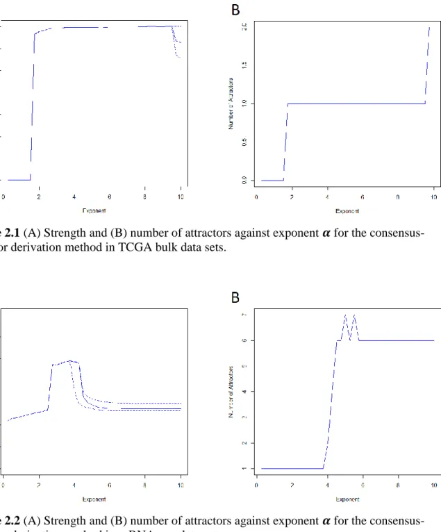
The results of this experiment suggest that the consensus-attractor derivation algorithm is

robust to the selection of exponent 𝛼. The strength of an attractor, defined as the tenth score of a

converged attractor [77] is stable in Figure 2.1A, where the ordinary curve is the median of the strengths of the ten attractors at the exponent and the dashed curves are the maximum and

minimum of the strengths. The number of distinct attractors remains 1 with regard to 𝛼 from 2 to

9 (Figure 2.1B), which presents that the consensus-attractor derivation method does not falsely divide the co-expressed genes associated with known biological processes into multiple sets

when 𝛼 is changed. Therefore, we set 𝛼 = 5 for consistency with the selection for the

(37)

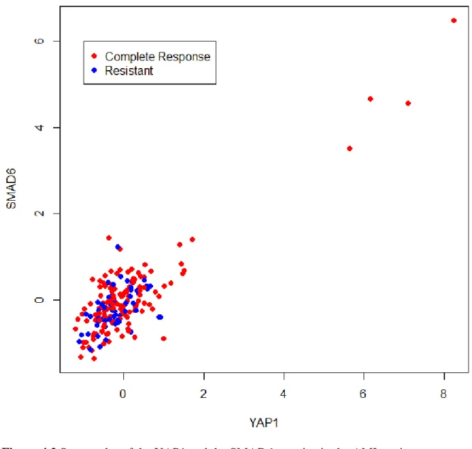
We conducted the same experiment that determines the parameter for the consensus method using single-cell gene-expression data sets which are described in Chapter 3 (Table 3.3) and mitosis genes from Table 3.4, were defined using scRNA-seq data sets, although they are almost identical to bulk mitosis genes. The mean duration for an attractor to achieve convergence is 2.06 minutes. The result of the experiment presents that the strength of an attractor, defined as the fifth largest score of the converged attractor for the weaker association in the scRNA-seq data,

decreases dramatically from 𝛼 = 4 (Figure 2.2A) and the number of distinct attractors increases

from 𝛼 = 4 (Figure 2.2B). Thus, for the scRNA-seq data, we set 𝛼 = 4 for the

(38)

Figure 2.1 (A) Strength and (B) number of attractors against exponent 𝜶 for the consensus-attractor derivation method in TCGA bulk data sets.

Figure 2.2 (A) Strength and (B) number of attractors against exponent 𝜶 for the

(39)

Summarization of the Derived Attractors

To perform a genome-wide study on transcriptomes in the data sets, we typically started the

attractor-derivation algorithm using all the 𝑛 features as seeds so the data set was “scanned” for

all possible attractors. As we discussed previously [77], initial attractors using different seeds

may converge at the same weight vector 𝐰, indicating a need for a procedure that identifies such

duplications. We propose a method that compares the top-ranked N features of the attractors by

the indices and decide if the two attractors can be categorized as one attractor. All attractors in 𝛀

are processed by the algorithm, and the resulting set of the attractors is 𝚲. If an incoming

attractor is different from all attractors that are in 𝚲, the new attractor is included as a new

member of 𝚲. The pseudocode of the algorithm is Algorithm 2.3. Compared with the previous

method [77], the method based only on the indices resolves the problem that when two attractors

converge to the same 𝐰 from different paths, the processes are stopped when their 𝐰 and 𝐦

remain different. In such cases, resulting attractors may not be considered the same using the previous method. For the experiment with multiple data sets, because the consensus-attractor derivation algorithm incorporates information from all data sets during the attractor-derivation process, it does not require a hierarchical clustering routine to create the “attractor clusters” from attractors with similar top-ranked genes from different data sets; thus, a virtual attractor can be inferred from the members of a cluster, which requires the assignment of arbitrary thresholds [77]. By contrast, consensus attractors are summarized using the same summarization algorithm as general attractors.

(40)

Algorithm 2.3

Require: Weights of the converged attractors 𝐰1, 𝐰2… 𝐰𝑞 ∈ 𝛀

Require: N: number of the features used in the evaluation

Require: 𝑠𝑜𝑟𝑡_𝑖𝑛𝑑𝑒𝑥(𝐰, N): The function that sorts 𝐰 in descending order and returns the indices of the top N

sorted elements. 𝚲 ← ∅ for each 𝐰i ∈ 𝛀 𝐯 ← sort_index(𝐰i, N) if 𝚲 ≠ ∅ and 𝐯 ∉ 𝚲 then 𝚲 ← 𝚲 ∪ 𝐯 else 𝚲 ← 𝐯 end if end for return 𝚲

Evaluation of the Significance of Multicancer Attractors in Individual Data Sets

Once consensus (multicancer) attractors were identified, we determined whether each was present in each of the individual cancer types by evaluating the corresponding statistical

significance. We used the hypergeometric test of the number of overlapped features with scores larger than 0.5 of the consensus attractor and the attractor in the individual data set. The size of the sampling population was the number of all features of the data set.

2.3 Implementation

Parallelization of the Algorithm

Because the number of features n is invariant for a particular data type, the bottleneck of the

algorithm is the evaluation of the associations, which is affected by the number of samples m,

and the upper bound of the complexity depends on the condition of convergence. Because the

scanning for all correlated patterns using a data set with 𝑛 features can be divided into 𝑛

attractor-derivation tasks, the process can be intuitively parallelized onto 𝑢 processing units,

(41)

executed on the clustered computing environment that is compatible with the Sun Grid system,

which automatically allocates 𝑛 tasks to the worker nodes of the cluster computer.

We deployed the program on the on-demand web service provided by Amazon called Amazon Elastic Compute Cloud (EC2) using a cluster-computing toolkit StarCluster

(http://web.mit.edu/stardev/cluster/). We launch the on-demand StarCluster using the Amazon Machine Image (AMI) with a preinstalled operating system and StarCluster (ami-3393a45a) on 20 m1.medium instances, such that multiple tasks with different running times are distributed on one working node to limit the number of idle nodes during the run.

We also implemented the algorithms for local workstations with multiple cores using the R

package doMC [89] to allocate tasks to the designated processors. Because doMC used the

fork-system call, the parallelized version of the implementation cannot be executed on Windows. The program was executed on Ubuntu 14.04 LTS on a Dell Precision T7610 workstation with Dual Intel Xeon Processor E5-2637 v2 (Four Core HT, 3.5 GHz) and 256 GB memory.

The attractor-derivation algorithms were mainly performed on the Amazon EC2 clusters. For scanning using the methylation data sets, we performed Step 2 locally due to the size of the data. The genomically localized algorithm is not parallelized because the complexity is much lower than other variations of attractor-derivation approaches.

2.4 Comparison with Previous Work

To validate the consensus algorithm, we compared the performance of the consensus-attractor derivation algorithm with the previous consensus-attractor method by applying algorithms on the 12 RNA-seq data sets of TCGA PanCan12 Data Freeze [47, 78] and analyzing the numbers of attractors discovered by the algorithms.

(42)

As presented in Table A.1, the consensus-attractor derivation method identified all seven gene-expression signatures that had been previously found using a combination of the attractor algorithm for an individual data set and hierarchical clustering, as in Table A.2, which is available under synapse ID syn1895985. In addition to known gene-expression attractors, the consensus-attractor derivation algorithm identified two novel attractors from the same data set.

For derivation of the WDR38 signature, because we eliminated gene WDR38 from data sets

COAD and READ, we applied the consensus-derivation algorithm on the ten TCGA data sets

with the gene. The top-ranked gene of the resulting attractor found using WDR38 as seed is

ZMYND10.

Comparison with Other Approaches

We compared the attractor-derivation method for individual data sets with K means, PCA, and hierarchical clustering quantitatively [77] and with ISA and ICA qualitatively [71]. For the clustering methods that accept multiple data sets as input, because CoCA [59], CoINcIDE [63], and iCluster [64] identify tumor subtypes across data sets, but the attractor-finding algorithm identifies co-expressed genes, they are not directly comparable. MDI [65] was developed to identify clusters of coregulated genes in multiple data sets, which is close to the aim of the consensus-attractor derivation algorithm, although inherently, the attractor-derivation method is not a clustering algorithm. Because MDI uses Gibbs sampling to estimate Dirichlet models, the output is not deterministic. However, the attractor-finding algorithm produces deterministic results. Because the output MDI and the consensus-attractor derivation algorithm relate qualitatively, we quantitatively compare their performances when capturing the coexpression events in the multiple data set.

(43)

Performances were assessed using six synthetic gene-expression data sets provided in the MDI software package. These data sets have 100 genes in seven patterns derived from the

time-series gene expression of the budding yeast S. cerevisiae. Because five of the six data sets were

derived from one of the six data sets, we compared the performances of the two methods using the similarity of clustering results withthat data set. We evaluated accuracy using the adjusted

Rand index (ARI) [90, 91] in the R package mclust [92, 93], which is an objective metric of the

similarity of two clustering results.

We applied the consensus-attractor method (Algorithm 2.2) on the six synthetic data sets

with 𝛼 = 5, 𝜖 = 10−5, and 𝑘 = 3. We sorted the consensus attractors using the third largest

score. From the attractor with the highest rank, we assigned the genes with scores > 0.5, > 0.4, > 0.3 to a cluster. Because the membership of attractors is not exclusive, a gene that is a member of two attractors was assigned to the cluster of the attractor with the higher rank. The attractor algorithm identified seven attractors, consistent with the design of the synthetic data sets. The resulting ARIs are 0.32, 0.36, and 0.33, respectively.

For the MDI approach, we performed MDI.m with the default 10,000 MCMC sampling

iterations and generated consensus clustering using GenerateClusteringPartition.m with one data

type and the fraction of samples from the beginning of the method’s sampling iterations that will be eliminated (“burn-in”) to reduce the dependence on the initial point = 0.3, 0.5, 0.7, 0.9. The resulting ARIs were 0.25, 0.25, 0.34, 0.34. For computational complexity, the consensus-attractor algorithm took 23.11 seconds to scan all 100 genes in the six data sets; MDI with 10,000 MCMC samplings took 14,171.58 seconds. The results suggested the consensus-attractor method and MDI achieve comparable accuracies when identifying patterns in multiple gene-expression data sets. However, the amount of computational complexity of the

(44)

consensus-attractor-finding algorithm is much lower than MDI, which is critical for an analysis using common human-gene-expression data sets, which typically have from 20,000 to 60,000 features. Therefore, the consensus-attractor algorithm performed equally well or better than MDI and outperformed MDI on complexity.