A New Fault Diagnosis Algorithm for Helical Gears Rotating at
Low Speed using an Optical encoder
Yimin Shao
1, Daizhong Su
2*, Amin Al-Habaibeh
3and Wennian Yu
11 State Key Laboratory of Mechanical Transmission, Chongqing University, Chongqing 400030,
People’s Republic of China
2 Advanced Design and Manufacturing Engineering Centre, School of Architecture, Design and the
Built Environment, Nottingham Trent University, UK
3 The Innovative and Sustainable Built Environment Technologies research group, School of
Architecture, Design and the Built Environment, Nottingham Trent University, UK
* Corresponding author, postal address: Professor Daizhong Su, Product Design, Nottingham Trent University, Burton Street, Nottingham, NG1 4BU, UK; E-mail address: [email protected];
Abstract
Helical gears are widely used in gearboxes due to its low noise and high load carrying capacity, but it is difficult to diagnose their early faults based on the signals produced by condition monitoring systems, particularly when the gears rotate at low speed. In this paper, a new concept of Root Mean Square (RMS) value calculation using angle domain signals within small angular ranges is proposed. With this concept, a new diagnosis algorithm based on the time pulses of an encoder is developed to overcome the difficulty of fault diagnosis for helical gears at low rotational speeds. In this proposed algorithm, both acceleration signals and encoder impulse signal are acquired at the same time. The sampling rate and data length in angular domain are determined based on the rotational speed and size of the gear. The vibration signals in angular domain are obtained by re-sampling the vibration signal of the gear in the time domain according to the encoder pulse signal. The fault features of the helical gear at low rotational speed are then obtained with reference to the RMS values in small angular ranges and the order tracking spectrum following the Angular Domain Synchronous Average processing (ADSA). The new algorithm is not only able to reduce the noise and improves the signal to noise ratio by the ADSA method, but also extracts the features of helical gear fault from the meshing position of the faulty gear teeth, hence overcoming the difficulty of fault diagnosis of helical gears rotating at low speed. The experimental results have shown that the new algorithm is more effective than traditional diagnosis methods. The paper concludes that the proposed helical gear fault diagnosis method based on time pulses of encoder algorithm provides a new means of helical gear fault detection and diagnosis.
Key Words: Machine condition monitoring; helical gear; low rotation speed gear; gear
fault diagnosis; encoder; angular domain synchronous averaging; RMS of angular domain
Journal title: Measurement, Publisher: Elsevier, DOI: 10.1016/j.measurement.2016.07.013, Available online: 5-JUL-2016, http://dx.doi.org/10.1016/j.measurement.2016.07.013
1 Introduction
Severalmethods exist in literature and in industry for gear fault diagnosis such as the time domain parameters method based on the variation of vibration amplitude (the RMS value, kurtosis, margin, etc.), the time domain synchronous averaging method based on the internal clock and the external clock, the modulation and demodulation analysis method based on the spectrum analysis, the adaptive-filtering method, the wavelet analysis method with transient nonlinear analysis, and the method of artificial intelligence.
Sajid et al.1 proposed an adaptive features extraction algorithm for real time gear fault
detection and integration of different techniques based on a combination of conventional one-dimensional and multi-dimensional search methods to detect faults in real time. Junsheng Cheng et al.2 put forward a gear fault diagnosis method based
on order tracking technique and local mean decomposition, which targeted the modulation feature of gear fault signal where fault characteristics found in gear fault signal were often related to the shaft’s revolution in the transient process. Ales Belsak and Joze Flasker 3 used a new family of bi-orthogonal wavelets to determine cracks in
gears, in which smoothness was controlled independently and discrete finite variation was used to optimise the synthesis bank. Roberto Ricci and Paolo Pennacchi4 studied
diagnostics of gear faults based on EMD and introduced a merit index that allowed the automatic selection of the intrinsic mode functions that should be used. F. Combet and L. Gelman5 applied the optimal de-noising filter based on the spectral kurtosis to
detect local tooth faults. Raja Hamzah6 studied the influence of operating condition on
acoustic emission (AE) generation during meshing of helical and spur gears.
The pattern classification is also found important in gear monitoring. Wilson Wang et al.7 developed an integrated classifier for gear system monitoring which was
performed by a neural fuzzy scheme. An online hybrid training technique was adopted based on recursive Levenberg-Marquet and least-squares estimate (LSE) algorithms to improve the classifier convergence and adaptive capability to accommodate different machinery conditions. H. Endo et al.8 presented a technique to differentially diagnose
two types of localized gear tooth faults, a spall and a crack in the gear, using a static analysis model to compare the changes in the kinematics of a meshing gear pair due to the two gear fault. N. Saravanan9 studied the use of discrete wavelets for feature
extraction and a Decision Tree for classification.
Monitoring of the evolution of fault severity is equally important. S. Loutridis10
presented a method for monitoring the evolution of gear faults based on the calculation of local energy density and the results showed that the local energy was a sensitive feature for assessing the fault magnitude and there was relationship between the energy content and the depth of the crack. S.J. Loutridis11 presented a method for
monitoring the evolution of gear faults based on empirical mode decomposition; and developed a theoretical model for a gear pair with a tooth root crack establishing an empirical law relating the energy content of the intrinsic modes to the crack magnitude. C.James Li and J.D. Limmer12 proposed a method that used linear dynamic modeling
to track the development of gear wear and tooth fatigue crack.
The existing methods, as outlined above, are not applicable to the fault diagnosis of low-speed helical gear, especially for the identification of early faults. There are two reasons: 1) the mesh impulse generated from the local fault on the gear is very small and the features are further difficult to be identified when coupled with the signals from shafts and bearings; 2) for the early stage of gear fault, local fault only occurs at one tooth or a few teeth, while other teeth are in normal meshing. In this case, differences can be only observed when the faulty teeth are in mesh action, and this tiny difference is easy to be covered by the noises generated from the normal vibration of the gear and bearing and other components making it difficult to be identified. Therefore, this work will address the way to accurately extract the feature signals of localized tooth faults, particularly the early fault characteristics of low-speed helical gear. In order to solve the problem, a new algorithm of angular domain sampling and feature extraction rules based on time impulses of encoder is proposed in this paper. Order tracking analysis based on the Angular Domain Asynchronous Averaging (ADSA) is introduced to detect the localized tooth faults in the very early stage for the low-speed helical gears, so that the maintenance can be readily performed before a catastrophic failure happens.
This paper consists of five parts: reviews of the research topics regarding the gear fault diagnosis where the motivation to form this paper is introduced. Then, the problem of helical gear fault diagnosis is formulated in the second section. The new algorithm of helical gear fault under the low rotation speed is introduced in section 3 and its experimental results and analysis results are outlined in section 4 which is followed by the conclusions in section 5.
2 Problem formulation
The currently used time series and angular domain sampling methods for determining fault features are all based on the analysis of the integral signal of gear mesh. In order to improve the diagnosis ratio of gear fault under a low rotation speed, the vibration mechanism of gear fault at different meshing positions must be investigated in detail. Figure 1 shows a schematic diagram of the normal and faulty mesh action of a helical gear pair. The meshing positions for the faulty tooth and normal tooth are represented by A and B respectively. It can be seen that, except for the faulty tooth, the other teeth of the large helical gear O1 will all be in normal meshing with their counterparts.
Figure 1: Schematic diagram of the normal and faulty mesh of pair of helical gears
Figure 2: Different positions for a faulty tooth in mesh
Figure 2 presents a detailed description of different positions when the faulty tooth is in mesh. Figure 3 shows the variation of the meshing stiffness. It is well known that there will be a localized reduction in the gear mesh stiffness Ks when the localized
faulty gear tooth (including tooth crack, pitting, spalls, etc.) comes into mesh, and this localized reduction in Ks leads to the changes of the dynamic response predicted by
the gear meshing dynamic model, as shown in Figure 4. The vibration characteristics are thus changes according to Eq. (1). If the changes of vibration arise from the normal meshing action, it is called regular vibration and is the main factor for gear vibration. If these changes of vibration are caused by the faulty teeth meshing, it is called abnormal gear vibration. The purpose of fault diagnosis is to identify this abnormal vibration. However, the associated vibration energy is very small and the vibration is always coupled with other motions, especially for a low-speed helical gear with large loading capacity.
To further understand the mesh and vibration characteristics of the faulty tooth, the generated impulse during the meshing process is studied using Figure 2. The local mesh positions for the faulty tooth in Figure 2 (a), (b) and (c) are represented by position 1, 2 and 3, respectively. It can be seen that the teeth are in single-edge contact for position 1 and 3, while are in double-edge contact for position 2. The mesh stiffness for position 1, 2 and 3 are also changes in the faulty area.
Figure 3: Variation of the gear mesh stiffness for a normal gear and a faulty gear
.Figure 4: Dynamic model of a pair of gears in mesh13
The governing equations of motion for the dynamic model shown in Figure 4 are:
{ 𝐽1𝜃̈1 + 𝑅𝑏1𝑐(𝑅𝑏1𝜃̇1− 𝑅𝑏2𝜃̇2− 𝑒̇) + 𝑅𝑏1𝑘𝑠(𝑅𝑏1𝜃1− 𝑅𝑏2𝜃2− 𝑒) = 𝑇1
𝐽2𝜃̈2− 𝑅𝑏2𝑐(𝑅𝑏1𝜃̇1− 𝑅𝑏2𝜃̇2− 𝑒̇) − 𝑅𝑏2𝑘𝑠(𝑅𝑏1𝜃1− 𝑅𝑏2𝜃2− 𝑒) = −𝑇2 (1) where J1 and J2 are the inertia moment of drive and driven gear respectively, Rb1 and
Rb2 are the base radius of drive and driven gear respectively, c is the damping ratio, θ1
and θ2 are the rotating angle of drive and driven gear respectively, Ks is the mesh
stiffness and e is the transmission error. The values of mesh stiffness Ks and
transmission error, e, change in the occurrence of gear fault.
From the above analysis, it can be seen that this is obviously different from the mechanism of abnormal vibration, which is induced only from faulty gear mesh. However, the existing time series sampling methods for determining fault features are all based on the analysis of the integral signal of gear mesh, hence this is one of the reasons for the difficult fault identification of low-speed helical gear. Although the angular sampling method can remove the nonlinearity of time series signal resulting from the variation of load and velocity, very little treatment of the relationship between sampling points in angular domain and faulty gear mesh is available. This is also the reason for the low performance of time scale and non-time scale angular
method in fault extraction.
3 A new fault diagnosis algorithm for helical gear rotating at
low speed
In this section, the calculation of the RMS values based on the physical structure of the gear using the encoder is introduced to improve the sensitivity in detecting faults in gears. Several other analyzing methods based on the angular-domain signal are intensively introduced.
3.1 Calculation of RMS values at small angular ranges in one revolution
The Root Mean Square (RMS), also known as virtual value, is a significant indicator to determine whether a mechanical system is working normally or not. It mainly reflects the energy of the signal, and has a high virtue of stability and repeatability. The formula of RMS is given as:
𝑋𝑅𝑀𝑆= √𝑁1∑𝑁𝑖=1𝑥𝑖2 (2)
where N is the total number of the sampling points for computation.
However the impulses caused by the gear’s fault would be thoroughly covered by the noise if N is much large, since there exists average process during the computation. As a result, the fault may not be correctly recognized in the RMS analysis.
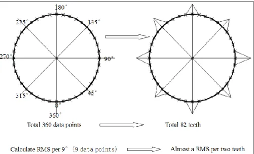
Figure 5: The specific process for calculating the RMS values
As we know, if the tooth pitting fault only occurs at only one tooth, the tooth pitting fault will lead to an impact per revolution, so if we calculate a RMS value per 360 degrees (i.e. 360 sampling points), the impact caused by tooth pitting may be concealed by the averaging process of RMS, which may lead to unobvious difference between normal and abnormal tooth. However if we calculate the RMS value at small angular ranges, then we may be able to find the impact caused by tooth pitting in a
revolution by focusing the analysis based on the physical structure of the gear. The number of point NRMS to perform averaging mainly depends on the angular-domain
sampling rate fa (S/r), the number of teeth for the faulty gear N2 (driven gear in this
study) and the desired number of points per teeth for RMS analysis Nteeth:
𝑁𝑅𝑀𝑆 = round(𝑁2∗𝑁𝑓𝑎
𝑡𝑒𝑒𝑡ℎ) (3)
where round() function rounds the value to the nearest integer. For example, if fa is
360S/r, N2 is 82, and Nteeth is 0.5 (meaning one point per two teeth), then the number
of point to perform RMS averaging analysis should be 9, which is about 9 degrees, as shown in Figure 5. The larger the Nteeth, the smaller the amount of angular range should
be chosen to perform the RMS analysis.
3.2 Refinement of the angular-domain signal based on pulse signal of an encoder
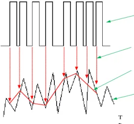
The angular-domain sampling is normally defined as the sampling that is directly triggered by the pulses produced by external devices. However, many useful information in the signal may be lost if the angular-domain sampling rate is too low, which may even cause a serious distortion of the signal. As a result, many factors should be considered in the setting of the angular-domain sampling rate based on the rotational speed. In order to satisfy the requirements, the angular domain sampling method is proposed based on pulses signal of an optical encoder. Firstly the aimed signals and the encoder’s signal are captured based on the internal clock. Secondly, the timing indexes (also called timing signal) of the rising edge for every impulse are calculated at the encoder’s signal following the original sampling. Finally, aimed signal is resample based on the timing signal so as to acquire the angular-domain signal. This method, as shown in Figure 6, is also called software sampling since the angular-domain signal is produced indirectly by internal re-sampling.
Figure 6: The angular-domain sampling
Generally, the angular-domain sampling rate (for resampling) is restricted by the
time-Encoder pulse signal Time-domain signal Angular-domain signal T Timing signal
domain sampling rate (for the original sampling) and the rotating speed of the shaft connected to the encoder, as shown below:
a t f n f 2 1 60 * (4)
where fa is the angular-domain sampling rate (S/r, Samples/revolution), n is the
rotating speed of the shaft connected with the encoder (rpm), and ft is the
time-domain sampling rate (S/s, Samples/second). The setting of the angular-time-domain sampling rate should satisfy inequality (4), or a comparatively large sampling error may exist during the resampling. In fact, this is achieved by interpolating the basic timing signal, which is acquired by calculating the timing indexes of the rising edge for every impulse in the encoder’s signal. For the software sampling, the angular-domain sampling rate could be flexibly adjusted and set.
3.3 ADSA method based on the angular domain re-sampling
The Angular Domain Asynchronous Averaging (ADSA), similar to the time synchronous averaging (TSA) algorithm, is an effective method for the extraction of periodic signal components from noisy signals. If there are deterministic periodic signals in the random signals, they can be picked up from the random, non-periodic signals or periodic signals with undesirable periods. This is achieved by superposition and averaging of the acquired signals whose length is determined by the angular displacement corresponding to a specified period Ф. The specified periodic component and its harmonics can be reserved by ADSA so as to improve the signal to noise ratio. The ADSA has also the advantage of being capable of performing the extraction even for the weak periodic signals in comparison to the traditional spectrum analysis methods.
Mathematically, assuming one signal, x(θ), consists of a periodic signal y(θ) and white noise signal n(θ), which reads:
𝑥(𝜃) = 𝑦(𝜃) + 𝑛(𝜃) (5)
Then the signal x(θ) is divided into N segments by the period of signal y(θ). And then superposition of these segments is carried out. Based on the irrelevance of the white noise, it can be described as:
𝑥(𝜃𝑖) = 𝑁𝑦(𝜃𝑖) + √𝑁𝑛(𝜃𝑖) (6)
Consequently, the output signal Y(θi) can be derived by averaging the signal x(θi) :
𝑌(𝜃𝑖) = 𝑦(𝜃𝑖) +𝑛(𝜃√𝑁𝑖) (7)
Therefore, the amplitude of the white noise in the output signal is reduced to √𝑁1 times of its original value, indicating that the ratio of the signal to its noise has been improved.
A huge merit for the ADSA method is that it can effectively reduce the noise contained in the signal and then improve the Signal to Noise Ratio (SNR). Therefore, because vibration signals normally contain significant noise, which can be considered as random signal which is generally normally distributed with mean of 0, in the averaging process, the influence of the noise could be reduced to 0 if only the number of the samples is relatively large. It should be noted that the ADSA method should be performed on the specified period Ф, meaning that if the faults are on the driving gear, then Ф should be the rotating period of the driving shaft so that any noise that is unrelated to the rotating frequency of driving shaft can be effectively removed. The proposed ADSA method can handle faults on any gear or on both gears as long as the corresponding encoder pulse signal is captured.
3.4 Order tracking analysis
For the angular-domain signal, the Nyquist sampling theory is as follows:
𝑂𝑆 < 2 ∗ 𝑂𝑚𝑎𝑥 (8)
where Os is the order sampling rate (same with fa, the angular-domain sampling rate),
and Omax is the maximum order of the signal.
For the angular-domain sampling, the order sampling rate Os is equal to the reciprocal
of the angular sampling interval, that is:
𝑂𝑆 = 𝛥1
𝜃 (9)
where Δθ is the angular interval of the angular sampling, and also the angular
resolution.
Similarly, the Discrete Fourier Transform (DFT) could also be applied in the conversion between angular-domain and order-domain. The formula of the DFT in the angular domain is same as the time domain, except that the meaning of the variable in the formula which is different, as shown below:
𝑋(𝑘) = ∑𝑁𝑛=1𝑥(𝑛)𝑒𝑗2𝜋𝑛𝑘𝑁 (10)
where x(n) is the nth sampling point in the angular-domain, X(k) is the kth point in the order-domain, and N is the number of points needed for the DFT.
In the order tracking spectrum analysis resulted from DFT, the largest order is Os/2,
and the number of points is N/2, hence the order resolution could be reflected as follows:
𝛥𝑂= 𝑅1 =𝑁∗Δ1
𝜃 (11)
Where ΔO is the order resolution in the order spectrum, R is the total revolutions for
the conversion, N is the number of points needs for the DFT, and Δθ is the angular
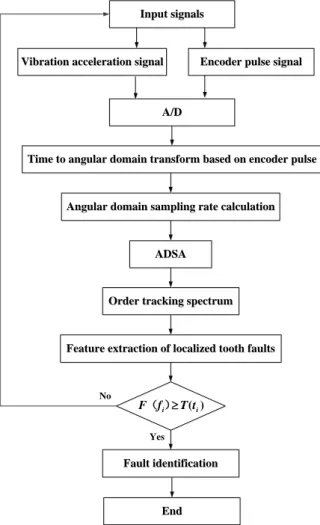
Figure 7 presents the complete flowchart of the proposed algorithm based on the angular-domain signal.
Input signals Input signals
Vibration acceleration signal
Vibration acceleration signal Encoder pulse signalEncoder pulse signal
A/D A/D
Time to angular domain transform based on encoder pulse Time to angular domain transform based on encoder pulse
Angular domain sampling rate calculation Angular domain sampling rate calculation
ADSA ADSA
Order tracking spectrum Order tracking spectrum
Feature extraction of localized tooth faults Feature extraction of localized tooth faults
) (i i Tt f F() Fault identification Fault identification End End Yes No
Figure 7: Flow chart of the proposed diagnostic algorithm
It should be noted that the proposed diagnostic method can be achieved only when a series of time-domain vibration signal and encoder pulse signal (i.e. N revolutions of the y(θ)) have been simultaneously collected so that the internal resampling (i.e. software sampling) can be conducted. This constitutes one of the major limitations of the proposed method. The larger the N, the more SNR can be achieved, and the more time are required to collect the time-domain signals before the analysis can be performed. However, it is possible that the proposed method can be run on the live data with a little time lag, which depends on N and the rotating speed ω of the faulty gear. For example, if N is 10 and the rotating speed of faulty helical gear is 750 rpm, then the time lag will be 0.8s.
4 Experimental results and discussions
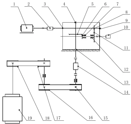
4.1 Experimental setupFigure 8: Diagram of test rig including the Encoder
Figure 8 presents the test rig with the encoder, which includes two stage gears and speed-increasing device by pulley structure. Component (1) is the driving motor, (2) is the speed and torque sensor, (3) is the tapered roller bearing, (4) is tapered roller bearing, (5,6) are spiral bevel gears, (7) is the tapered roller bearing, (8,11) are helical gears, (9) is the tapered roller bearing, (10) is the encoder, (12) is tapered roller bearing, (13) is tapered roller bearing, (14) is speed and torque sensor, (15,16) is the level 1 pulley of lifting speed, (17, 18) are the level 2 pulley of lifting speed and (18) is the loading motor.
Two acceleration sensors are installed on the housing of bearing at the position 3 and 9 in Figure 8, and an encoder 10 has been assembled on the test rig to achieve the angular-domain sampling.
Figure 9: The data acquisition system
1 2 3 4 5 6 7 8 9 10 11 12 13 14 15 16 17 18 19 Accelerometer 1 Accelerometer 2 Accelerometer 3 Power Supply Coupler Kistler 5134B DAQ NI USB-6259 Cumputer
The data acquisition system is shown in Figure 9. The data acquisition is conducted using National Instrument NI USB-6259 with LabVIEW software.
There are total six conditions of tooth surface in the helical gear 11 to be investigated: one healthy condition and five faulty conditions. The faulty conditions are based on the area ratio of pitting on the surface of the helical for 0%, 25%, 50%, 75% and 90%. Another faulty condition is tooth broken. The different pitting sizes of gear’s tooth surface and the tooth broken are shown in Figures 10. In the test, the rotating speeds of the faulty helical gear are set to 28 rpm, 210 rpm, 350 rpm, 500 rpm and 750 rpm respectively, the load torques are set to 2 N.m, 4 N.m, 6 N.m and 8 N.m respectively.
(a) 25%-pitting area (b) 50%-pitting area
(e) Broken tooth (c) 75%-pitting area (d) 90%-pitting area
Figure 10: The investigated pitting faults of the helical gear and broken tooth
4.2 Fault features of helical gear
In order to investigate the fault features of the helical gear under different sampling rates of angular-domain signal, the typical fault signal of broken tooth is implemented. The picture of tooth broken is shown in Figure 10(e). The test is conducted under the input rotational speed of 210 rpm and load torque of 8 Nm. The time-domain sampling rate is set to 25600Hz, and the angular-domain sampling frequency is set to 360, 1800 and 3600 (r/s) respectively.
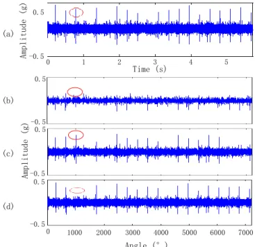
Figure 11 (a) presents an example of an original faulty signal of the helical gear in time-domain. The impulse from the meshing of the faulty gear in time-domain is obvious. In order to investigate the effectiveness of the angular-domain sampling rate for fault waveform features of angular domain, the original fault signal of helical gear in time-domain is transferred into the angular-time-domain by resampling the signal based on time pulses of the encoder. Figures 11 (b), (c) and (d) show the angular-domain waveforms with sampling rate of 360, 1800 and 3600 S/r respectively. Notice that the angular-domain waveform gets closer to the original time-angular-domain waveform with the increase
of the angular-domain rate. For example, the impulse at about 1000° is completely missed in Figure 11 (b) because of the low angular-domain sampling rate. However, Figures 11 (c) and (d) clearly show this impulse.
Figure 11: The comparison of the waveforms
(a) Time-domain waveform (b) Angular-domain waveform at 360 S/r (c) Angular-domain waveform at 1800 S/r (d) Angular-domain waveform at 3600 S/r
Figure 12: The comparison of the refined waveforms
(a) Time-domain waveform (b) Angular-domain waveform at 360 S/r (c) Angular-domain waveform at 1800 S/r (d) Angular-domain waveform at 3600 S/r
Figures 12 (a) – (d) are zoomed waveforms of Figures 11 (a) – (d), which reflect the impulse features in detail when the broken tooth ran into and out of the mesh zone. These abrupt impulses results from the sudden localized decrease of the gear mesh
0 1 2 3 4 5 -0.5 0.5 -0.5 0.5 -0.5 0.5 -0.5 0.5 Time (s) 0 1000 2000 3000 4000 5000 Angle (°) 6000 7000 A m p l i t u d e ( g ) A m p l i t u d e ( g ) (a) (b) (c) (d) 5.078 -0.4 0.4 -0.4 0.4 -0.4 0.4 -0.4 0.4 Time (s) 6400 Angle (°) 6410 A m p l i t u d e ( g ) A m p l i t u d e ( g ) (a) (b) (c) (d) 5.085
stiffness when the broken tooth ran into the mesh zone. The results are the same as the analyzed results in section 2. As a result, with the load constant, the vibration would abruptly increase so much to form an impulse, and return to normal when the broken tooth runs out of the mesh zone. Figures 12 (c) and (d) reflect this whole phenomenon in great detail, which shows the refined angular-domain waveforms get closer to the shape of refined time-domain waveform. Hence, the lost information decreases with the increase of the angular-domain sampling rate.
4.3 Fault feature identification of helical gear
4.3.1 Order tracking spectrum based on the ADSA method
Figures 13, 14 and 15 are the order tracking spectrum based on the ADSA method for every revolution (N=1) from normal condition, 25%-pitting area and 90%-pitting area when the rotating speed is 210 rpm and load torque is 2 Nm. Figure 13 and 14 show, especially for the 90%-pitting area, that the vibration energy is mainly concentrated on 82th order and 1/2 time order and 2 time order for the pitting damage, which is precisely the number of the tooth of the faulty gear.
As to normal condition, no such phenomenon happens in Figure 15. Since the same features exist in Figures 13 and 14, which have higher resolution, the order tracking analysis based on the ADSA method is almost perfect in distinguishing between the 90%-pitting damage and the normal condition. For the 25%-pitting damage, the differentiation is not that clear.
Figure 13: Order tracking spectrum of 25% pitting fault using the ADSA
0.12 0 Order (n) Am pl it ud e (g ) 20 40 60 80 100 120 140 160 180 0.1 0 0.02 0.04 0.06 0.08
Figure 14: Order tracking spectrum of 90% pitting fault using the ADSA
Figure 15: Order tracking spectrum of normal gear condition using the ADSA
0.14 0 Order (n) A m p l i t u d e ( g ) 20 40 60 80 100 120 140 160 180 0.1 0 0.02 0.04 0.06 0.08 0.12 0.10 0 Order (n) A m p l i t u d e ( g ) 20 40 60 80 100 120 140 160 180 0 0.04 0.06 0.08 0.02
4.3.2 RMS value in small angular ranges
Figure 16: The RMS curves under different angular ranges
(a) 180 degrees (b) 72 degrees (c) 9 degrees
Figure 16 is the RMS curves in different angular ranges (180, 72 and 9 degrees) under the tooth broken fault. When in 180 degrees, no obvious impulse exists in the curves. For every revolution, there exists only one impulse, which is easily recognized that the impulses are just caused by the breakage in the tooth. Therefore, the RMS curves become clearer as the decrease of angular ranges. The result has shown that the analysis method of RMS values of small angular ranges is effective for the identification of helical gear fault under low rotational speed.
(a) (b)
Figure 17: The RMS values of small angular ranges for pitting fault of helical gear
0 1 2 3 4 5 0.01 0.05 0.05 0.1 0.01 0 0 5 10 Rotation (r) A m p l i t u d e ( g ) A m p l i t u d e ( g ) (a) (b) (c) 15 20 A m p l i t u d e ( g ) 0 Angle (°) A m p l i t u d e ( g ) 1000 2000 3000 6000 2 4000 5000 4 6 8 10 0 Normal 25%-pitting 0 Angle (°) A m p l i t u d e ( g ) 1000 2000 3000 6000 2 4000 5000 4 6 8 10 0 Normal 90%-pitting
Figure 17 shows that the RMS values of small angular ranges (45 degrees) in one revolution for pitting fault of the helical gear under the rotation speed of 56 rpm. The RMS values of 25% and 90% pitting fault are higher that of the normal condition, and the RMS values of 90% are higher than the values of 25% pitting fault. The results have shown that RMS value of small angular range is effective statistical parameter for the identification of helical gear fault under low rotational speed.
4.4 Comparison with traditional method
4.4.1 Improve the Signal to Noise Ratio
Figure 18 shows the angular domain waveforms of 90% pitting fault in the helical gear when the rotating speed is 210 rpm and the load is 4 Nm. The impulse waveform cannot be found in this case (i.e. when the ADSA method is not used to process the data). Figure 19 shows the angular domain waveforms of 90% pitting fault in the helical gear after using ADSA when the rotating speed is 210 rpm and load is 4 Nm. The impulse can be seen clearly, which means the impulses are precisely caused by the abrupt change of the mesh stiffness when fault tooth ran into the mesh zone. The cyclic impulses duo to the fault are not significantly clear in this case, as in waveform without using ADSA, which means its Signal to Noise Ratio (SNR) is much lower. Therefore, the ADSA has improved the Signal to Noise Ratio under the heavy environment noise, and it is effective to improve the success ratio of helical gear fault.
Figure 18: The waveform of angular domain sampling without ADSA
Figure 19: The waveform of angular domain sampling using ADSA
4.4.2 Improve the success ratio of helical gear fault diagnosis
Figure 20 shows the order tracking spectrum of 25% pitting fault without using the
0 Angle (°) A m p l i t u d e ( g ) 100 200 0 -0.02 300 400 500 600 700 0.02 0.04 0 Angle (°) A m p l i t u d e ( g ) 100 200 0 -0.02 300 400 500 600 700 0.04 0.02 0.06
ADSA, when the rotating speed is 210 rpm and load torque is 2 Nm (same as Figure 13). There are many peaks in Figure 20 which makes it difficult to identify the fault. This is because the vibration energy is not mainly concentrated at 82th order and 1/2 time order and 2 time order for the pitting damage. Therefore, the ADSA method makes the vibration energy more concentrated at some specific orders.
Figure 20: Order tracking spectrum of 25% pitting fault without using the ADSA
4.4.3 Envelop analysis based on the Hilbert Transform
The envelop analysis based on the Hilbert Transform can demodulate the gear vibration signal and reveal the information of the amplitude modulation that may exist in the signal; it is basic analysis method for gear fault diagnosis.
Figure 21: Time domain waveform when the helical gear fault is 90% pitting fault under rotational speed of 210 rpm and 2 Nm load
Figure 21 is the time domain waveform when the helical gear fault is 90% pitting fault under rotational speed of 210 rpm and 2 Nm load (same as Figure 14). Figure 22 is the envelop spectrum of Figure 21. Although meshing frequency (287Hz) of gear exists, the side band frequencies are not clear in Figure 22 and the amplitude of meshing frequency is also small in Figure 22. Comparing with the results in Figure 14, it can be concluded that Order tracking spectrum based on ADSA is much more powerful in identifying the fault of the helical gear than the envelop analysis based on the Hilbert Transform 0 Order (n) A m p l i t u d e ( g ) 20 40 0 80 100 140 160 180 0.04 0.02 0.14 60 120 0.12 0.10 0.08 0.06 0 Time (s) A m p l i t u d e ( g ) 0.5 1 -0.5 2 0.5 0 1.5 1
Figure 22: Envelop spectrum of Figure when the helical gear fault is 90% pitting fault under rotational speed 210rpm and load of 2Nm
4.4.4 RMS value under different angular ranges
Figure 23 presents a comparison between the RMS values under different angular ranges with pitting area of 50%, rotational speed of 210 rpm and toque of 2Nm. The meshing impact due to the fault of the gear can be found when the RMS calculation use the data of per-angular-45o (per 45 degrees angular range), but the meshing
impact due to the fault of the gear is not clear if the data of per-angular-360o is used.
The result has shown that the RMS value calculation method of small angular ranges at one revolution is more effective than traditional RMS calculation methods.
Figure 23: Comparison between the RMS values under different angular ranges
0 Frequency (Hz) A m p l i t u d e ( g ) 100 200 0 600 500 300 400 1 2 3 4 5 ×10³ 0.08 Revolution (r) Am pl it ud e ( g) 0 0.02 0.04 0.06 0 1 2 3 RMS per 45° RMS per 360°
5 Conclusions
Helical gear box generates vibration signals with strong noise and non-stationary characteristics in the time domain. This causes difficulties when attempting to diagnose helical gear tooth initial faults features (e.g. tooth crack, pitting, spalls etc.) using vibration signals, especially when the gears are running at the low speed
To cope with these difficulties, a new diagnostic algorithm based on the Order tracking analysis and the ADSA method, as well as the new concept of RMS value calculation in small angular ranges, is introduced to detect the localized tooth faults in the very early stage for the low-speed helical gears. Compared with the traditional method, the proposed method has been found to effectively improve the ability and success rate of the helical gear fault diagnosis based on the experimental work provided in this study.
One limitation of the proposed diagnostic algorithm is that there will be a time lag before it is performed on the live data, especially when the gears are running at a low speed range. Another limitation is that the proposed algorithm is not fully capable to differentiate different types of localized tooth faults. However, the order tracking spectrum may provide some insights about it, which will be the focus of the future research.
The proposed diagnostic system (as shown in Figure 9 ) can be used in many industrial applications, such as the end of line test for a gear manufacture, condition monitoring for the gearbox inside the agitators, wind turbines, automobiles etc.
Acknowledgement
The authors are grateful for the financial support provided by the European Commission under the FP7 Marie Curie International Incoming Fellowship programme, FP7-PEOPLE-2009-IIF (Marie Curie) project No. 253403, and the financial support provided by the National Natural Science Key Foundation of China (grant number 51035008).
References
1. Hussain S and Gabbar HA. A novel method for real time gear fault detection based on pulse shape analysis, Mechanical Systems and Signal Processing 25 (2011): 1287–1298
2. Junsheng Cheng, Kang Zhang and Yu Yang. An order tracking technique for the gear fault diagnosis using local mean decomposition method,Mechanism and Machine Theory 55 (2012): 67–76
3. Belsak A and Flasker J. Determining cracks in gears using adaptive wavelet transform approach,Engineering Failure Analysis 17 (2010): 664–671
4. Ricci Rand Pennacchi P. Diagnostics of gear faults based on EMD and automatic selection of intrinsic mode functions,Mechanical Systems and Signal Processing 25 (2011): 821–838
5. Combet F and Gelman L. Optimal filtering of gear signals for early damage detection based on the spectral kurtosis, Mechanical Systems and Signal Processing 23 (2009): 652–668
6. Raja Hamzah RI and Mba D. The influence of operating condition on acoustic emission (AE) generation during meshing of helical and spur gear, Tribology International 42 (2009): 3– 14
7. Wang W and Kanneg D. An integrated classifier for gear system monitoring, Mechanical Systems and Signal Processing 23 (2009): 1298–1312
8. Endo H, Randall RB and Gosselin C. Differential diagnosis of spall vs. cracks in the gear tooth fillet region: Experimental validation,Mechanical Systems and Signal Processing 23 (2009): 636–651
9. Saravanan N and Ramachandran KI. Fault diagnosis of spur bevel gear box using discrete wavelet features and Decision Tree classification, Expert Systems with Applications 36 (2009): 9564–9573
10.Loutridis S. A local energy density methodology for monitoring the evolution of gear faults, NDT & E International 37 (2004): 447–453
11.Loutridis SJ. Damage detection in gear systems using empirical mode decomposition,Engineering Structures 26 (2004): 1833–1841
12.Li CJ and Limmer JD. Model-based condition index for tracking gear wear and fatigue damage, Wear 241 2000: 26–32
13.Kahraman A and Singh R. Non-linear dynamics of a spur gear pair, J. Sound and Vibration, 142(1) (1990): 49-75.