Mining Mid-level Features for Image Classification
Basura Fernando, Elisa Fromont, Tinne Tuytelaars
To cite this version:
Basura Fernando, Elisa Fromont, Tinne Tuytelaars. Mining Mid-level Features for Image
Clas-sification. International Journal of Computer Vision, Springer Verlag, 2014, 108 (3), pp.186-203.
<
10.1007/s11263-014-0700-1
>
.
<
hal-00968299
>
HAL Id: hal-00968299
https://hal.archives-ouvertes.fr/hal-00968299
Submitted on 31 Mar 2014
HAL
is a multi-disciplinary open access
archive for the deposit and dissemination of
sci-entific research documents, whether they are
pub-lished or not.
The documents may come from
teaching and research institutions in France or
abroad, or from public or private research centers.
L’archive ouverte pluridisciplinaire
HAL, est
destin´
ee au d´
epˆ
ot et `
a la diffusion de documents
scientifiques de niveau recherche, publi´
es ou non,
´
emanant des ´
etablissements d’enseignement et de
recherche fran¸cais ou ´
etrangers, des laboratoires
publics ou priv´
es.
(will be inserted by the editor)
Mining Mid-level Features for Image Classification
Basura Fernando · Elisa Fromont ·Tinne Tuytelaars
Received: date / Accepted: date
Abstract Mid-level or semi-local features learnt using class-level information are potentially more distinctive than the traditional low-level local features constructed in a purely bottom-up fashion. At the same time they preserve some of the robustness properties with respect to occlusions and image clutter. In this paper we propose a new and effective scheme for extracting mid-level features for image classification, based on relevant pattern mining. In par-ticular, we mine relevant patterns of local compositions of densely sampled low-level features. We refer to the new set of obtained patterns as Frequent Local Histograms or FLHs. During this process, we pay special attention to keeping all the local histogram information and to selecting the most relevant reduced set of FLH patterns for classification. The careful choice of the visual primitives and an extension to exploit both local and global spatial information allow us to build powerful bag-of-FLH-based image representations. We show that thesebag-of-FLHs are more discriminative than traditional bag-of-words and yield state-of-the-art results on various image classification benchmarks, including Pascal VOC.
Keywords Frequent itemset mining· Image classification · Discriminative patterns·Mid-level features.
1 Introduction
Vector quantized local features, be it densely sampled or extracted from inter-est points, have a proven track record in vision. They are the default image representation for a wide variety of applications ranging from image retrieval
B. Fernando, T. Tuytelaars
KU Leuven, ESAT-PSI, iMinds Belgium E. Fromont
Universit´e de Lyon, Universit´e de St-Etienne F-42000, UMR CNRS 5516, Laboratoire Hubert-Curien, France
to image classification. Although early papers presented them as a kind of au-tomatically discovered object parts (e.g. wheels of airplanes) [42], they have, in practice, only limited semantic meaning in spite of what the name visual words suggests.
Based on this observation, some recent works [6, 14, 22, 26, 39, 41] have looked into the construction of more distinctive,mid-level features(sometimes also re-ferred to assemi-local featuresorparts). Some of them operate in a strongly su-pervised setting (e.g. poselets [5]), while others use only weak supervision (i.e. no annotations at the parts-level, only at class-level), e.g. hyperfeatures [1], discriminative patches [41] or blocks that shout [22]. Here we focus on the weakly supervised case (which, by the way, has been shown to outperform the strongly supervised case [22]).
A first set of methods (e.g. [6, 14, 22]) starts from the same description that proved its value for local features, building on robust gradient-based represen-tations such as HoG [13]. The main difference lies in the fact that for mid-level features, typically larger (or actually, more detailed) patches are used com-pared to those used traditionally for local features. This makes them more in-formative, so potentially more distinctive. However, this also makes them more sensitive to misalignments, deformations, occlusions, parts not falling entirely on a single surface or object, etc. Simply clustering such larger patches, as done for local features, does not work very well under these circumstances. Besides, existing iterative clustering approaches are not guaranteed to converge to the global optimum and depend on the initial seeds. If the deformations are big, it is not clear that the resulting patches in the clusters are indeed uniform in appearance (as we also observed in our experiments). Instead, typical vari-ations in appearance of the mid-level features need to be learned, e.g. using exemplar SVMs as done in [22, 41]. However, these methods also start with an initial clustering or nearest neighbour search, which again limits them to cases with not too big deformations. Object parts close to an object boundary, (self-)occlusion or orientation discontinuity are not likely to be found with these methods.
Moreover, HoG patches are rigid. For small patches (local features), this is often a reasonable approximation, as shown by the success of SIFT [29]. However, with the patches becoming larger, the rigidity of HoG makes the features very specific. They seem to lack the necessary flexibility needed to cope with the observed deformations, be it due to viewpoint changes or due to within-class variability.
A second set of methods (e.g. [1, 40]) builds on more robust representations typically used for global object or scene descriptions, such as bag-of-words [12] or Fisher Vectors [33]. Representing a mid-level feature based on the distribu-tion of the local features it contains, brings the necessary flexibility to cope with deformations. In the work of Agarwal and Triggs [1], mid-level features are represented with local bag-of-words, which are then clustered to obtain a set of mid-level vector-quantized features. Simonyan et al. [40] do the same for Fisher Vectors, and further add a global discriminative dimensionality re-duction step. In both cases, the link between the mid-level feature and the
low-level features composing it, is lost in the final representation. Moreover, for neither of these methods the construction of mid-level features is selective: if some low-level features inside the mid-level patch fall on the background or turn out to be unstable, they cannot be ignored, adding noise to the overall process.
Finally, some methods (e.g. [27, 28, 10, 37, 49, 51]) have looked at construct-ing mid-level features by combinconstruct-ing multiple low-level features. However, this quickly brings combinatorial problems, and seemed not that successful in prac-tice. Moreover, combinations have been limited to relatively few elements (usu-ally pairs or triplets).
In this paper, we propose a new method to extract mid-level features, build-ing on the extensive pattern minbuild-ing literature and expertise. Mid-level features are constructed from local bag-of-words (LBOW, as e.g. used in [1, 35, 43, 53]) representing the distribution of local features in a semi-local neighbourhood. However, we do not keep the full bag-of-words, but select subsets of low-level features, that are optimal in terms of discriminativity, representativity, and non-redundancy. We refer to the resulting mid-level features asFrequent Local Histogramsor FLHs. Each FLH is composed of a set of low-level visual words that are spatially close. Compositions are not restricted to pairs or triplets, as in [10, 27, 28, 37], but can easily contain ten or more elements. Since we focus only on the number of these elements within a local image area, ignoring their spatial configuration, the resulting representation is very flexible and can cope well with various types of image deformations, occlusions and image clutter. Moreover, being constructed from standard low-level features (visual words), they can be indexed efficiently, as we show in [19]. From all sets of visual words that co-occur frequently, we select the final set of FLHs based on their discriminativity for the classification task at hand, their non-redundancy as well as their representativity. While the data mining techniques we apply are rather standard, we adapt them to our specific setting aiming at mid-level visual features that yield good results on various image classification tasks.
Even though frequent itemset mining techniques and variants thereof are well-established in the data-mining community [3, 45], they are, to date, not commonly used in state-of-the-art image classification methods. This is sur-prising, since it has been shown that these mining methods allow the con-struction of high-level sets of compound features which can, in many cases, capture more discriminative information [9]. Nevertheless, most attempts so far applying pattern mining to image classification [31, 50, 35, 53] were not able to demonstrate competitive results on standard datasets. Here, we propose an effective scheme for applying pattern mining to image classification by adapt-ing the generic pattern minadapt-ing tools to the specific context of visual features extracted from images. We provide an extensive analysis of parameter selec-tion and relevant pattern mining. We compare several spatial pyramid schemes which capture both local and global spatial information with and without data mining, and we highlight some advantages of mining-based approaches that capture local spatial information compared to non-mining methods.
Fig. 1: FLH mining and image representation process. First dense SIFT de-scriptors are extracted. Each descriptor is assigned to a visual word (hard assignment). For each dense descriptor, its K spatial nearest neighbors are selected (in practice, we use all local descriptors within a squaren×n neigh-bourhood). From these descriptors a local bag-of-words (LBOW) representa-tion is created for each dense point. Then we mine for the most frequent local histograms from the entire dataset. These frequent local histograms are known as FLH patterns or just FLHs. Afterwards, using a post processing step, we select the most suitable set of FLHs for image classification. We encode the LBOWs in an image using these relevant FLH patterns (but note that some of the LBOWs won’t be captured by any of the selected FLH patterns). Finally by counting how many times each FLH pattern is used to encode an image, we create a bag-of-FLHs representation.
The composition of the following three aspects makes our method differ-ent from earlier approaches that apply pattern mining to bag-of-visual-words (noted BOW in the rest of the paper): i) we start from local BOW (LBOW) to capture local information, ii) we take particular care in loosing as few informa-tion as possible during the conversion step necessary to transform a histogram (LBOW) into a suitable input for a mining algorithm (known as atransaction) and iii) we carefully but automatically select the relevant and non redundant patterns that will be used in our classification step. Thebag-of-FLHs creation process is shown and explained in the caption of Fig. 1.
This paper extends our earlier work [18] with more details about our mo-tivations and related works as well as more extensive experimental validation. In particular, we added experiments comparing our approach to non-mining ones and combining FLH and Fisher vectors, which led to very good results.
The rest of the paper is organized as follows. First, we review related work in section 2. Section 3 provides details on the construction of relevant FLHs and shows how they can be used for image classification. In Section 4 we show how local and global spatial information can be combined. Section 5 describes the experimental validation, demonstrating the power of our method for challenging image classification problems. In Section 6 we compare FLH with state-of-the-art methods. Section 7 concludes the paper.
2 Related work
Frequent pattern mining techniques have been used to tackle a variety of computer vision problems, including image classification [23, 31, 53, 54], action recognition [20, 34], scene understanding [50], object recognition and object-part detection [35]. Aobject-part from the application, these methods mostly differ in the image representation used, the way they convert the original image representation into a transactional description suitable for pattern mining techniques and the way they select relevant or discriminative patterns. We therefore organize our discussion on related works along these three axes. We end with a discussion of other methods for extracting mid-level features.
Image representations: A standard image representation nowadays is the bag-of-visual words [12]. The BOW can be computed either globally or locally in a neighborhood around an interest point (LBOW). In the context of pat-tern mining-based image classification, local bag-of-words are usually preferred (e.g. in [23, 34, 35, 43, 53]), since they result in sparse representations, a better signal-to-noise ratio, an increased robustness to image clutter and some low level spatial information (proximity). Spatial configuration mining based on LBOW was first shown by Quacket al. [35], although they did not use these configurations for classification. Perhaps, the distinctive feature configurations mined in their work were too specific, making them less suited for image clas-sification. Secondly, they only relied on interest points to create object specific transactions. In contrast, FLH uses dense sampling (which captures a larger amount of statistics) and relevant pattern mining to find not just frequent but rather discriminative image representations. More structured patterns such as sequences and graphs capturing the spatial distribution of visual words have been used by [31], while [52] uses boosting on top of binary sets of visual words discovered by pattern mining. Gilbertet al. [20] have applied itemset mining to action recognition using rather primitive features like corners, while in [54] high level features such as attributes [16] are successfully used with mining techniques. In [50], Yaoet al.present a structured image representation called
group-lets. To find discriminative group-lets, they mine for class-based associa-tion rules. Associaassocia-tion rule learning [2] is used for discovering relaassocia-tions between variables using different measures of interestingness. Class-based association rules are used to find relations between itemsets and class variables. Itemsets that are highly associated with class variables are selected as patterns.
However, none of the above representations took a particular care both in designing a suitable encoding to effectively use pattern mining for image classification and, in designing a dedicated post-processing step to obtain state-of-the-art classification results on standard image classification datasets.
Transforming bags to transactions: Most existing mining methods simply use individual visual words as items in a transaction. Transactions are created in such a way that if a visual word is present in the histogram, then it is also present in the transaction (i.e. itemset). Information on the exact frequency, i.e. how often the visual word occurred in the LBOW, is lost in this process. In [23], Kimet al.use a new representation called Bag-to-set (B2S) to trans-form a histogram into a transactional trans-form without losing intrans-formation. In this approach, each bin of the histogram is converted into a sequence of binary digits. The length of this sequence is given by the largest value that a specific bin can take. For example, if the maximum value for the first bin of a set of histograms is 5 and in a particular histogram, this first bin has the value 3, its B2S representation will be [11100] (the length of the sequence is 5 and only the 3 first values are “true”). Afterwards, B2S concatenates all the sequences (from all the bins in the histogram), transforming the histogram into a binary se-quence that can be regarded as a “transaction” by a traditional pattern miner. The B2S representation is, to our knowledge, the only unsupervised effort to explicitly avoid information loss in the conversion to transactions. However the mining phase might generate artificial visual patterns (ghost patterns) that do not exist in the image database (see Fig. 2 for an example of such ghost pat-terns). For example, this encoding implies that when a histogram bit has some particular valuex, all the values lower thanxare also true at the same time in the binary encoding. This could result in wrong possible matching as shown for pattern c(1) in Fig. 2. Besides, a pattern could incorporate parts of a bin description (for example the first and last ”1” without the middle ones) that would have no ”real” meaning according to the original encoding. These ghost patterns hinder the performance of the patterns constructed using the B2S method.
Alternatively, one could give each visual word a weight depending on how many times it appears in the histogram and apply weighted itemset min-ing [55]. However, this method only postpones the loss of information as it then simply sums all the itemset weights to discover patterns. FLH, as pro-posed in this paper, avoids information loss without generating unexisting patterns, as the number of occurrences of a visual word must match exactly.
Mining relevant patterns: Frequent patterns can be more discriminative than individual features (e.g. visual words), since a pattern is a combination of
sev-W1 W2 W3 W4 W5 0 0,5 1 1,5 2 W1 W2 W3 W4 W5 0 0,5 1 1,5 2 W1 W2 W3 W4 W5 0 0,5 1 1,5 2 W1 W2 W3 W4 W5 0 0,5 1 1,5 2 W1 W2 W3 W4 W5 0 0,5 1 1,5 2 W1 W2 W3 W4 W5 0 0,5 1 1,5 2 W1 W2 W3 W4 W5 0 0,5 1 1,5 2 W1 W2 W3 W4 W5 0 0,5 1 1,5 2 W1 W2 W3 W4 W5 0 0,5 1 1,5 2
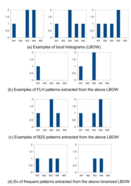
(a) Examples of local histograms (LBOW).
(b) Examples of FLH patterns extracted from the above LBOW
(c) Examples of B2S patterns extracted from the above LBOW
(d) Ex of frequent patterns extracted from the above binarized LBOW
Fig. 2: Three different transaction creation methods and resulting patterns. For all the figures, the X axis shows the different visual words and the Y axis gives the value of the histogram bin for each visual words. (a) represents some local histograms. (b) shows some resulting FLH patterns extracted from the histograms in (a). (c) shows some patterns extracted using the B2S approach. (d) shows some patterns extracted from binarized histograms. Both FLH and B2S do not lose any information during the transaction construction stage. However, B2S generates some patterns that would be mapped to non existing data which we call ghost patterns. For example, (c1), the first B2S pattern (Fig. (c) first pattern) would be mapped to the first and second local histograms ((a1) and (a2)). Nevertheless, (a1) should not be mapped to (c1) as the word frequencies of W4 do not match.
eral primitives and therefore likely to capture more distinctive information. However, when using local bag-of-words to create transactions as we plan to do, each source (image) generates multiple transactions and a pattern that is found only in a relatively small number of images can still be frequent if it appears in really high numbers within this small set of images. Applying stan-dard relevant pattern discovery methods under these circumstances, as done in [20, 35, 50, 53], may not be the best strategy. Most of the methods that use pattern mining in the context of image classification are restricted to stan-dard class-based association rules [2], stanstan-dard discriminative pattern mining approaches [20, 25, 35, 50, 53] or other supervised methods such as boosting to find interesting patterns [31, 52]. In [53], Yuanet al.present a visual pattern mining algorithm based on a likelihood ratio test to find relevant patterns in an unsupervised manner. None of these works considers the issue of repet-itive structures in images, causing frequent yet not representative patterns. Therefore, for a pattern to be useful it should be both discriminative and representative.
Mid-level feature extraction: As mentioned already in the introduction, other methods have been proposed to extract mid-level features using compositions of low-level features. However, most of them are limited to the use of pairs or triplets of features [10, 27, 28, 37]. Only a few have used higher-order statis-tics (co-occurrence of visual words), albeit on a single image [49] or pairs of images [51] only. Unlike pattern mining, they do not exploit database-wide statistics.
Early work on extracting mid-level features are the hyper-features of Agar-wal and Triggs [1]. Like us, they start from local-bag-of-words butclusterthem recursively (in a hierarchical fashion) to find a new set of spatial features called hyper-features. Then they represent each image as a bag-of-hyper-features. In our work, FLH patterns are constructed from local histograms in which sub-histograms are mined as patterns instead of clustering entire local sub-histograms. While the approach of [1] also captures larger patterns, it does not have the same flexibility in local geometry as our scheme.
Boureau et al. [6] have proposed to construct macro-features by jointly encoding a small neighbourhood of SIFT descriptors from a 2×2 or 3×3 square. As in the case of hyper-features, this method cannot selectively add a patch (SIFT descriptor) to the macro-feature. In contrast, in our FLH approach, each patch in the local neighborhood is selected to be included in a pattern only if it satisfies certain criteria (such as frequency, discriminativity, redundancy etc.). As a result, and in contrast to [6], FLH patterns are robust to spatial deformations, occlusions and image clutter.
In [41], Singhet al.start with HoG templates and try to find discriminative and representative patches using a clustering and a support vector machine-based approach. Unfortunately, there is no guarantee on the cluster purity or the class-based representativeness of the clusters. Nevertheless, empirically this method manages to converge to a set of reasonable clusters. In a similar spirit, Junejaet al. [22] learn parts incrementally, starting from a single part
occurrence with an exemplar SVM and gradually adding more examples after an alignment step. As mentioned earlier, we believe that starting from a rigid HoG representation does not allow sufficient flexibility and makes the parts too specific. We take a different approach and build more general (in the sense of more flexible) mid-level features as compositions of several local rigid SIFT features. It turns out the tradeoff between rigidity at a local scale and flexibility at a level scale) is an important parameter when building mid-level features (e.g. by changing the size of the local SIFT features).
Our approach exploits thelocalstatistics of an image while methods such as Fisher vector-based approaches [21] exploit zero, first and second orderglobal
statistics of an image [33, 8]. Consequently, as shown in the experiments, our method is complementary to Fisher vector encoding. Recently, Simonyan et al. [40] have proposed Deep Fisher Networks, that apply the Fisher vector encoding at a semi-local scale. Integrating Fisher vectors in our framework in a similar fashion, is an interesting research direction we plan to investigate in the near future.
3 FLH-based Image Representation and Classification
After introducing some notations, we explain how we mine frequent local his-tograms (FLHs) (section 3.1). We then show how we select the most relevant set of FLHs for image classification (section 3.2) and present a suitable kernel for relevant pattern-based image classification (section 3.3).
Each image Iis described by a set of features{fi|i= 1. . . nI} and a class
labelc,c∈ {1. . . C}. We assume that all the descriptors have been clustered to obtain a set of so-called visual words. Then, each key pointfi is given a label
wi ∈ W known as the visual word index. |W| is the visual word dictionary
size. In our approach, for each feature fi we compute alocal histogram (also
called a local bag-of-words LBOW), xi ∈ N|W| using the K spatial nearest
neighbours offi (based on the distance between image coordinates and also
including fi itself as a neighbour). In practice, we use all features within a
local square neighbourhood of sizen×naround the feature. The set of all the local histogramsxi created from all images is denoted byΩ.
3.1 Frequent local histogram mining
Items, Transactions and Frequencies: In order to avoid loss of information during the transaction creation process without generating ghost patterns, we propose the following new definition of anitem. An item is defined as a pair (w, s),w∈W ands∈N, with sbeing the frequency of the visual wordw in
the local histogram. Note that 0< s ≤K and for a given image there is at most one item per histogram bin.
Next, we create the set oftransactions Xfrom the set of local histogramsΩ. For eachx∈Ωthere is one transactionx(i.e. a set of items). This transaction
xcontains all the items (wj, sj) such that the bin corresponding towj inxhas
the nonzero valuesj. Alocal histogram pattern is an itemsett⊆Γ, whereΓ
represents the set of all possible items. For any local histogram patternt, we define the set of transactions that include the patternt,X(t) ={x∈X|t⊆x}. The frequency of t is |X(t)|, also known as the support of the pattern t or
supp(t).
Frequent Local Histogram: For a given constantT, also known as the minimum support threshold, a local histogram pattern t is frequent if supp(t)≥ T. A patternt is said to beclosed if there exists no patternt0 such thatt⊂t0 and
supp(t)=supp(t’).
The set of frequent closed patterns is a compact representation of the frequent patterns (i.e we can derive all the frequent patterns from the closed frequent ones). In this work we refer to a frequent and closed local histogram pattern as aFrequent Local Histogram orFLH.Υ is the set of all FLHs.
FLH Mining: Given the set of transactionsX, we can use any existing frequent mining algorithm to find the set of FLHsΥ. What is specific to our method is that i) the input of our algorithm is a set of local histogramsΩ, and ii) a preprocessing step is performed building the set of transactions X from the local histogramsxi as described above. Items (wk, sk) in a transaction x∈X
can then be regarded as standard items in itemset mining.
The problems of finding these frequent itemsets are fundamental in data mining, and depending on the applications, fast implementations for solv-ing the problems are needed. In our work, we use the optimised LCM al-gorithm [45]. LCM uses a prefix preserving closure extension to completely enumerate closed itemsets. This allows counting the support of an itemset efficiently during the mining process.
The LCM algorithm [45] supports database reduction, so that it can handle dense traditional datasets in short time and computes frequencies in linear time. It includes a strong pruning method to further reduce the computation time when the number of large frequent itemsets is small. It also generates closed itemsets with no duplication. For all these reasons, LCM is preferred over the well-known APRIORI algorithm [3]. Note though that the outcome does not depend on the choice of mining algorithm.
Encoding a new image with FLHs: Given a new image, we extract features by dense sampling and assign them to visual words. For each feature, we compute a LBOW around it, considering its K spatial nearest neighbours. Given this LBOW x, we convert it into a transactionxand check for each FLH pattern
t ∈ Υ whether t ⊆ x. If t ⊆ x is true, then x is an instance of the FLH pattern t. The frequency of a pattern t in a given image Ij (i.e., the number
of instances oftin Ij) is denoted asF(t|Ij). We again refer to figure 1 for an
3.2 Finding the best FLHs for image classification
We want to use the FLH setΥas a new set of mid-level features to represent an image. To this end, we first need to select the most useful FLH patterns from
Υ because i) the number of generated FLH patterns is huge (several millions) and ii) not all discovered FLH patterns are equally relevant for the image classification task. Usually, relevant pattern mining methods select patterns that are discriminative and not redundant. On top of that, we introduce a new selection criterion, representativity, that takes into account that, when using LBOW, a single image generates multiple transactions. As a result, some patterns may be frequent and considered discriminative but they may occur in very few images (e.g. due to repetitive structures). We believe that such features are not representative and therefore not the best choice for image classification. A good FLH pattern should be at the same time discriminative, representative and non-redundant. In this section we discuss how we select such patterns.
Relevance criterion: We use two criteria for pattern relevance: a discrimina-tivity scoreD(t) [9] and a newrepresentativity scoreO(t).
The overall relevance of a patterntis denoted by S(t) defined as:
S(t) =D(t)×O(t) (1)
We claim that if a patternthas a high relevance scoreS(t), it is likely to be discriminative and repeatable across images, hence suitable for classification.
Discriminativity score: To find discriminative patterns, we follow the entropy-based approach of [9], where a discriminativity scoreD(t) (0≤D(t)≤1) for a patterntis defined as:
D(t) = 1 +
P
cp(c|t)·logp(c|t)
logC , (2)
with p(c|t) the probability of class c given the pattern t, computed as follows: p(c|t) = PN j=1F(t|Ij)·p(c|Ij) PN j=1F(t|Ij) . (3)
Here,Ijis thejthimage andN is the total number of images in the dataset.
p(c|I) = 1 if the class label ofIj is c and 0 otherwise. A high value of D(t)
implies that the patterntoccurs only in very few classes. Note that in Eq. 2, the term logC is used to make sure that 0≤D(t)≤1.
Representativity score: The second factor for the relevance S(t) is the repre-sentativityO(t). To compute it, we compare the distribution of the patterns over all the images with the optimal distribution with respect to a classc. A pattern having an optimal distribution is called an optimal pattern and de-noted by t∗
c for class c. This optimal distribution is such that i) the pattern
occurs only in images of classc, i.e.p(c|t∗
c) = 1 (giving also a discriminativity
score of 1), and ii) the pattern instances are equally distributed among all the images of classc, i.e.∀Ij, Ik in classc,p(Ij|t∗c) =p(Ik|t∗c) = (1/Nc) whereNc
is the number of images of classc.
To find patterns with distributions close to the optimal one, we define the
representativity scoreof a patterntdenoted byO(t). It considers the divergence between the optimal distribution for class c p(I|t∗c) and the distribution for patterntp(I|t), and then takes the best match over all classes:
O(t) = max
c (exp{−[DKL(p(I|t
∗
c)||p(I|t))]}) (4)
whereDKL(.||.) is the Kullback-Leibler divergence between two distributions.
The quantity p(I|t) is computed empirically from the frequencies F(t|Ij) of
the pattern t:
p(I|t) = PF(t|I)
jF(t|Ij)
(5)
Redundant patterns: We propose to remove redundant patterns in order to obtain a compact representative set of FLHs. We take a similar approach as in [48] to find affinity between patterns. Two patternstands∈Υ are redundant if they follow similar document distributions, i.e ifp(I|t)≈p(I|s)≈p(I|{t, s}) wherep(I|{t, s}) gives the document distribution given both patterns{t, s}.
p(I|{t, s}) =PF(t|I) +F(s|I)
jF(t|Ij) +F(s|Ij)
(6)
We define the redundancyR(s, t) between two patternss, tas follows:
R(s, t) = exp{−[p(t)·DKL(p(I|t)||p(I|{t, s}))+p(s)·DKL(p(I|s)||p(I|{t, s}))]}
(7) where p(t) is the probability of pattern t:
p(t) = P IjF(t|Ij) P tj∈Υ P IjF(tj|Ij) (8)
Note that 0 ≤R(s, t)≤1 and R(s, t) = R(t, s). For redundant patterns,
DKL(p(I|t)||p(I|t, s))≈ DKL(p(I|s)||p(I|t, s))≈ 0 which increases the value
Finding the most suitable patterns for classification: We are interested in find-ing the most suitable pattern subsetχ where χ⊂Υ for classification. To do this we define the gain of a patternt denoted byG(t) s.t.t /∈χ andt∈Υ as follows:
G(t) =S(t)−maxs∈χ{R(s, t)·min(S(t), S(s))} (9)
In Eq. 9, a pattern t has a higher gain G(t) if it has a higher relevance
S(t) (i.e. it is discriminative and representative) and if the pattern t is non redundant with any patternsin setχ(i.e. R(s,t) is small). To find the bestk
patterns we use the following greedy process. First we add the most relevant pattern to the relevant pattern setχ. Then we search for the pattern with the highest gain (non redundant but relevant) and add this pattern into the setχ
untilk patterns are added (or until no more relevant patterns can be found).
3.3 Kernel function for effective pattern classification
After computing the k most relevant and non-redundant FLHs, we can rep-resent each image using a new reprep-resentation calledbag-of-FLHs by counting the occurrences of such FLHs in the image. LetLbe such a bag-of-FLHs for the imageIL andM be thebag-of-FLHs for the imageIM. We propose to use
the kernel function
K(L, M) =X
i
min(pL(i),pM(i)) (10) to find the similarities between thebag-of-FLHs ofL andM. HereL(i) is the frequency of theithselected pattern in histogramL. This kernel provides
good classification accuracies for our frequent pattern-based image representa-tion. It is a standard histogram intersection kernel but with non-linear weight-ing. This reduces the importance of highly frequent patterns and is necessary since there is a large variability in pattern frequencies. Similar power-low nor-malization methods are used in improved Fisher Vector-based methods [33, 11].
4 GRID-FLH: Incorporating global spatial information to FLH
Finally, we propose a variant of bag-of-FLHs that incorporates both global and local spatial information. We build on the spatial pyramid idea [24] and apply it in our FLH mining framework. First we create LBOW for all features in the image. Then we discover grid-specific relevant FLH patterns by employing the process described in Section 3.2. For each image, we concatenate these grid-specificbag-of-FLH representations to create a new representation called
GRID-FLH. TheGRID-FLH is a more structured local-global representation with more flexibility than traditional spatial pyramids [24]. Note that we mine FLHs specific to a grid cell from all the images and then create a bag-of-FLHs
in a grid specific way. As a result each grid-cell uses a different set of FLH patterns.
5 Experimental Setup and Evaluations
First, we introduce the datasets used to evaluate ourF LH-based method in section 5.1. Then, we compare our method with the most relevant baselines in section 5.2 using some default parameters (standard SIFT descriptors with a dictionary size of 200 visual words and transactions created using 5 spatial neighbours). In section 5.3, we analyze our parameters and design choices. In section 5.4, we demonstrate on the importance of the selection of the most relevant patterns and the use of an appropriate kernel. In section 5.5 we per-form some experiments to evaluate the effect of our choices (in particular of our chosen parameters) for standard BOW-based methods. In section 5.6 we evaluate the effect of our parameters on the mining step. Finally, in section 5.7 we evaluate the GRID-FLH extension.
5.1 Datasets and evaluation criteria
We evaluate the newbag-of-FLH (hereafter denoted by just FLH) approach on several challenging natural image datasets:GRAZ-01 [32],Oxford-Flowers17[30],
15-Scenes [24],Land-Use [49] and thePASCAL-VOC2007 dataset [15]. The GRAZ-01 dataset consists of two object classes (bike and person) and a complex yet representative background class. For each object class (bike or person) we randomly sample 100 negative images (50 from the background class and 50 from the other object class) and 100 positive images, as done in [24]. The Oxford-Flowers dataset contains 17 flower categories where each category contains 80 images. We randomly select 60 images from each category for training and 20 images for testing as in [30]. The 15-Scenes dataset contains 15 scene categories. This dataset is useful for evaluating scene classification. From each scene category, 100 randomly selected images are used for training and the rest are used for testing as in [24]. The Pascal-VOC-2007 dataset consists of 20 object classes and 9,963 images. This dataset is one of the most interesting image classification benchmarks. The data has been split into 50% for training/validation and 50% for testing. Land-Use [49] is a new dataset consisting of 2100 images of area imagery of various urban areas. There are 21 classes including various spatial structures and homogeneous textures. For this dataset, we also keep 50% of the images for training and 50% for testing. We use classification accuracy to evaluate our results on the Oxford-Flower and Land-Use datasets and the mean classification accuracy computed over per-class-based classification accuracies for the 15-scenes dataset as done in the literature (and for comparison purpose). For the GRAZ-01 dataset we report ROC equal error rate. For the Pascal-VOC-2007 dataset, we report the mean average precision or mAP. Because of the size of the Pascal-VOC-2007 and Land-Use datasets, we did not perform any baseline comparisons nor
parameter optimizations for them, we simply report the results obtained with the parameters optimized for the other datasets.
For the initial baseline experiments (and for all datasets), we start from SIFT descriptors [29] densely sampled over the image with patches of size 16×16 pixels and a grid spacing of 8 pixels.
We use the K-means algorithm to create the visual dictionaries and LIB-SVM [7]1 to train an SVM. We use the square root intersection kernel for
FLH-based methods as presented in Section 3.3.
5.2 Initial comparison with baseline methods
We compare ourFLH-based method using some default settings (spatial neigh-borhood size K=5, standard SIFT, dictionary size of 200) with BOW-based image classification, spatial pyramid matching(SPM)[24], visual word-based standard frequent itemset mining with binarized local bag-of-words (denoted byFIM) and with the B2S [23] representation. For all baseline methods, we use the same LCM algorithm for pattern mining and an intersection kernel for SVM. We use a maximum of 10.000 patterns for all mining methods. We also report results for the mining-based method combined with BOW using an average Kernel (denoted by BOW+Mining-Method). The results are shown in Table 1.
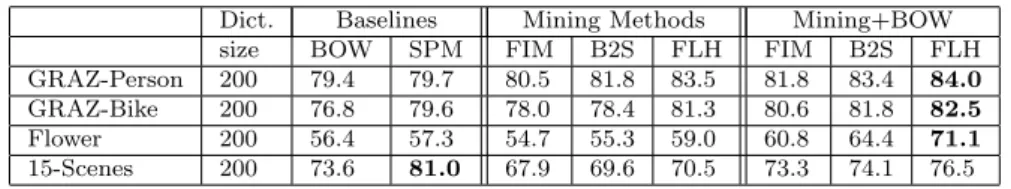
Table 1: Comparison with baseline methods. Classification accuracies are re-ported for GRAZ-01, Oxford-Flower17 and 15-Scenes datasets with a local neighborhood size of K=5.
Dict. Baselines Mining Methods Mining+BOW
size BOW SPM FIM B2S FLH FIM B2S FLH
GRAZ-Person 200 79.4 79.7 80.5 81.8 83.5 81.8 83.4 84.0 GRAZ-Bike 200 76.8 79.6 78.0 78.4 81.3 80.6 81.8 82.5 Flower 200 56.4 57.3 54.7 55.3 59.0 60.8 64.4 71.1 15-Scenes 200 73.6 81.0 67.9 69.6 70.5 73.3 74.1 76.5
FIM is comparable with SPM (except for 15-Scenes) while B2S (which is an alternative lossless histogram transformation approach as explained in Sec-tion 2) slightly outperforms FIM. TheFLH-based method outperforms all the baseline methods as well as all the other mining-based methods, except in the 15-Scenes dataset. This result shows the importance of not losing information during the transaction creation time. We believe that our FLH-based method improves the results over B2S because it does not generate artificial visual patterns (i.e. patterns not actually present in the data set) while B2S does. The combination ofBOWs andbag-of-FLHs gives better results compared to all other methods and is an indication of the complementary nature of both
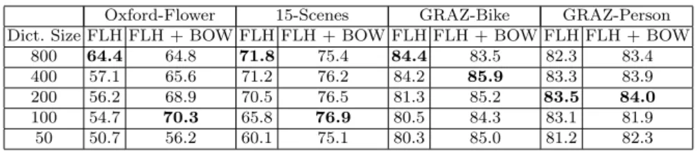
Table 2: The effect of dictionary size on FLH-based methods using SIFT-128. Classification accuracy on training data using cross-validation.
Oxford-Flower 15-Scenes GRAZ-Bike GRAZ-Person Dict. Size FLH FLH + BOW FLH FLH + BOW FLH FLH + BOW FLH FLH + BOW
800 64.4 64.8 71.8 75.4 84.4 83.5 82.3 83.4
400 57.1 65.6 71.2 76.2 84.2 85.9 83.3 83.9
200 56.2 68.9 70.5 76.5 81.3 85.2 83.5 84.0
100 54.7 70.3 65.8 76.9 80.5 84.3 83.1 81.9
50 50.7 56.2 60.1 75.1 80.3 85.0 81.2 82.3
representations. Especially the improvement for the Flowers dataset is remark-able. FLH outperforms other baselines for GRAZ-01 dataset as well. For the 15-Scenes dataset (with the default parameters) spatial pyramids and even just BOW outperform the other methods. These initial experiments, without parameter optimization, already clearly hint at the power of our new image representation.
5.3 Parameter selection and optimization
In this set of experiments we analyze the effect of several parameters of our method: dictionary size, SIFT feature size, and local neighborhood size. We use a three-fold cross-validation on training data to optimize our parameters using Oxford-Flower, 15-Scenes and GRAZ-01 datasets.
In the remaining experiments (sections 5.4, 5.5, 5.6 and 6), we then use the found optimal parameters to test our FLH-based methods on the test sets.
Dictionary size: We are interested in exploiting local spatial information us-ing minus-ing methods. Larger visual dictionaries may restrict the possibility of exploiting co-occurring local statistics. To evaluate this phenomenon we eval-uate the effect of the dictionary size on our FLH-based method. We report results for FLH and FLH+BOW with different dictionary sizes (Table 2). Note that when combiningFLH andBOW we do not reduce the dictionary size for BOW, but always use a dictionary size of 800, as large dictionaries have proven to perform better for BOW. Results decrease when the dictio-nary size is reduced. However, the results improve with reduced dictionaries for FLH+BOW, up to some level. This indicates that with a smaller dictio-nary size (up to some level)FLHscomplementarity withBOW representation increases.
Smaller dictionaries reduce the discriminativity of the visual primitives. However, this does not seem to affect the discriminativity of the FLH patterns, which may even become more robust and stable when combined with BOW. Therefore, smaller dictionaries created using even less discriminative features might be better suited forFLH. This is tested in the next experiment.
70 80 90 100 110 120 130 70 80 90 100 110 120 130 70 80 90 100 110 120 130 70 80 90 100 110 120 130
Fig. 3: Spatial bining of SIFT32 (left) vs SIFT128 (right)
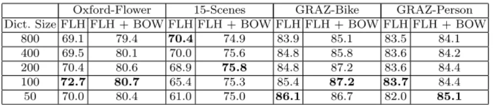
Table 3: Effect of SIFT-32 features on FLH. Classification accuracy on training data using cross-validation.
Oxford-Flower 15-Scenes GRAZ-Bike GRAZ-Person Dict. Size FLH FLH + BOW FLH FLH + BOW FLH FLH + BOW FLH FLH + BOW
800 69.1 79.4 70.4 74.9 83.9 85.1 83.5 84.1
400 69.5 80.1 70.0 75.6 84.8 85.8 83.6 84.2
200 70.4 80.6 68.9 75.8 84.8 87.2 83.6 84.4
100 72.7 80.7 65.4 75.3 85.4 87.2 83.7 84.4
50 70.0 80.4 61.0 75.0 86.1 86.7 82.0 85.1
Less discriminative features: We evaluate the effect of less discriminative fea-tures onFLH using the same four datasets and local neighborhood size of 5 (Table 3). For this we useSIF T32 features that are extracted like the stan-dard SIFT (referred to asSIF T128) but performing spatial binning of (2×2) instead of (4×4) (See Fig.3). Results are shown in Table 3, for FLH with SIFT32 by itself, as well as when combined withBOW (using SIFT128 and a 800 dimensional vocabulary for the BOW). For most of the settings, we obtain better results on all datasets except 15-Scenes, when compared to the case of SIFT-128.
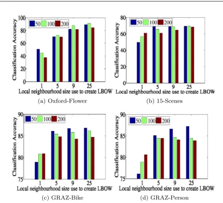
Larger local neighborhoods: The use of smaller dictionaries and less discrim-inative SIFT features allows the FLH-based method to exploit larger neigh-borhoods. To evaluate this relation, we run some further experiments on the same datasets – see Fig. 4. The best results are obtained when reducing both SIFT feature size and dictionary size while increasing the neighborhood size of the local spatial histograms. For Oxford-flower, the best classification accu-racy obtained with SIFT features is 91.0% for a dictionary size of 100 words,
SIF T32 features and a neighborhood size of 25. A similar trend is observed for 15-Scenes dataset and the GRAZ dataset. Note that this is a larger neigh-borhood size (covering up to 48×48 pixels) than what is typically used in the literature [53, 20].
We can conclude that theFLH-based method obtains its best results when exploiting larger patterns with smaller dictionaries and less discriminative primitive features.
From now on, for allFLH-based experiments we use the SIFT32 descriptor and a neighborhood size of 25 neighbors. On average best performance is
(a) Oxford-Flower (b) 15-Scenes
(c) GRAZ-Bike (d) GRAZ-Person
Fig. 4: Effect of neighborhood size (K, horizontal axis), dictionary size (color coded) and SIFT-32 on classification accuracy for the (a) Oxford-Flower (b)15-Scenes (c) GRAZ-Bike (d) GRAZ-Person on training data using cross-validation.
obtained around 100 visual words or less for most of the datasets. As a result hereafter we use a visual dictionary size of 100 words.
5.4 Effect of relevant pattern mining and of the kernel functions
FLH mining algorithms can generate a large number of FLH patterns (in our case, 1-20 million) before the relevant pattern mining step. Therefore, we select the most relevant-non-redundant ones, as described in Section 3.2. Here we evaluate the importance of this pattern selection step by compar-ing different criteria: the most frequent (Frq.), the most representative-non-redundant (Rps.)(eq. 4), the most discriminative-non-representative-non-redundant (Disc.)(eq.2) and the most relevant-non-redundant (Rel.) (i.e. representative, discriminative and non-redundant) patterns (see Table 4). We always select the top 10.000 patterns for each criterion which we believe is sufficient to obtain good results. These results clearly show that only selecting the top-k most frequent patterns (as often done in computer vision literature, e.g. [31]) is not a good choice for classification. Both representativity and discriminativity criteria alone also do
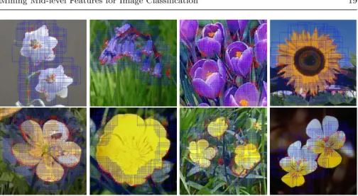
Fig. 5: FLH patterns using SIFT32 where each red dot represents the central location and the blue square represents the size of the FLH pattern. Each pattern is generated from a 48×48 pixel image patch. In this region there are 25 features each covering a 16×16 pixel patch and overlapping 50% with their neighbors. Note how the relevant non-redundant patterns seem to capture most of the relevant shape information in the images.
not provide the best results. It’s the relevant non-redundant FLH patterns that are the most suitable for classification.
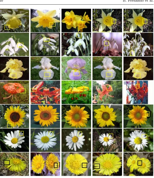
Some of these relevant and non-redundant FLH patterns are shown in Fig. 5. These selected most relevant FLH patterns seem to capture most of the relevant shape information in an image. In Fig. 6 we show the most rel-evant pattern for seven different flower categories. Note how each relrel-evant pattern captures several local feature configurations. All these configurations seem visually similar, even though they show quite some variability as well, especially when compared to the mid-level features obtained by methods that start from a rigid HoG-based representation.
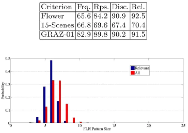
As can be seen from Fig. 5, these FLH patterns cover relatively large regions. Fig. 7 shows the distribution of pattern size. Most of the pattern sizes are between length 5 to 8. This implies that most of the local histogram patterns consist of 5-8 non-zero components. Very large patterns and very small patterns have very low probability. The relevant-non redundant patterns contain slightly less items.
In Table 5, we evaluate the effect of the square root intersection kernel using relevant non-redundantFLH patterns onOxford-Flower,GRAZ-01 and
15-Scenes datasets. The proposed square-root weighting increases the classi-fication accuracy for all datasets, both when using the linear kernel and the non-linear intersection kernel.
The square-root intersection kernel combines an intersection kernel and a power kernel with power 0.5. Both kernels decrease the impact of very
fre-Fig. 6: Each row represents the most relevant FLH pattern for a given flower category. Note the flexibility of our representation. While it’s always the same FLH pattern, the appearance of the corresponding patches varies a lot.
quent patterns. As shown by experiments, this kernel is better than either kernel separately (see Table 5). This shows that the intersection kernel and power kernel with power 0.5 do not reduce sufficiently the influence of frequent patterns. An alternative would be to use a smaller power than 0.5, (e.g. 0.25). The main advantage of this is that the power kernel can be implemented as a simple normalization of the features. Efficient linear classifiers can be used subsequently as opposed to costly non-linear classifiers. We plan to investigate this effect in our future work.
Table 4: Effect of relevant pattern mining on classification performance using FLH
Criterion Frq. Rps. Disc. Rel. Flower 65.6 84.2 90.9 92.5 15-Scenes 66.8 69.6 67.4 70.4 GRAZ-01 82.9 89.8 90.2 91.5
Fig. 7: The distribution of the pattern size
Table 5: Effect of the kernel on classification performance using FLH
K(x,y) =x·yt √x·√ytP imin(xi,yi)Pimin( √ xi, √ yi) Flower 89.5 92.0 91.2 92.5 15-Scenes 68.0 68.9 69.0 70.4 GRAZ-01 88.5 89.5 89.8 91.5
Table 6: Effect of larger patches (48×48) and dictionary size on BOW/SPM based image classification.
Oxford-Flower 15-Scenes GRAZ-Bike GRAZ-Person Dict. Size BOW SPM BOW SPM BOW SPM BOW SPM
100 55.0 60.8 66.5 73.7 79.5 83.0 79.5 80.0 1000 62.9 66.5 72.1 76.4 80.0 80.0 83.0 83.0 4000 65.5 67.4 72.9 76.2 79.0 80.5 83.0 82.5
5.5 Effect of larger patches and dictionary size on BOW based image classification
One might argue that the FLH-based method with the optimized parameters described in the previous section outperforms the BOW baseline because of the use of larger patches and much simpler features. To evaluate this hypoth-esis, we perform another experiment using BOW with SIFT-32 descriptors extracted from large patches of size 48×48 pixels. By varying the dictionary size we evaluate the performance of the BOW and SPM methods. The results are shown in Table 6. They show that just increasing the patch size of SIFT de-scriptors is not sufficient to increase the classification accuracy for BOW-based methods. For example forOxford-Flower dataset the best performance using SPM is 67.4% while FLH reported 92.5%. For 15-Scenes datasetF LH+BOW
5.6 Effect of larger spatial neighborhoods and smaller dictionary size on frequent pattern based image classification
To evaluate the effect of larger spatial neighborhoods and smaller visual dic-tionaries on all pattern-based methods (i.e. FIM, B2S and FLH) we perform another experiment using SIFT-32 descriptors. Transactions are created us-ing a spatial neighborhood size of 25 neighbors. Results are shown in Fig. 8. We report results using both histogram intersection kernel (Ints.) and square root histogram intersection kernel (Sqrt. Ints.). For all three methods (FIM, B2S and FLH), the traditional top-k most frequent pattern selection method performs poorly. All methods benefit from the relevant pattern selection but the FLH-based method benefits the most (the top-k most frequent pattern results are improved by 27% while it is 19% for B2S and 17% for FIM for Oxford-Flower). A similar trend can be observed for the other datasets too. It is clear from this experiment that smaller visual dictionaries that are con-structed from less discriminative SIFT are only helpful if we use the relevant pattern selection step. Since the binary histogram transformation used in the FIM method loses some valuable information, this method does not benefit that much from the relevant pattern selection step nor from the reduction of the dictionary size, SIFT dimension and the increase of the spatial neighbor-hood. We believe that the significant 10% improvement (on Oxford-Flower) of FLH over B2S when using the same parameters is due to two reasons; (1) FLH local representation is more expressive and explicit compared to B2S, (2) FLH does not generate artificial patterns (ghost patterns).
5.7 Effect of GRID-FLH vs Spatial pyramids
In this section we compare the extension of bag-of-FLHs called GRID-FLH introduced in section 4. We compare GRID-FLH with FLH and spatial pyra-mids [24] with BOW BOW) and spatial pyrapyra-mids with FLH (SPM-FLH). SPM-BOW is the standard spatial pyramids applied over BOW while in SPM-FLH spatial pyramids are computed over bag-of-FLHs. Results are reported in Table 7. GRID-FLH consistently improves over FLH and spatial pyramid variants (both SPM-BOW and SPM-FLH). Especially in scene clas-sification the improvement obtained by GRID-FLH is significant.
Table 7: Effect of GRID-FLH vs Spatial pyramids
Method FLH SPM-BOW SPM-FLH GRID-FLH Flower 92.5 57.3 92.6 92.9 15-Scenes 70.4 81.0 82.8 86.2 GRAZ-01 91.6 84.3 92.4 93.8
Top−K Frq. Ints. Rel. Ints. Rel. (Sqrt. Ints.) 50 60 70 80 90 FIM B2S FLH (a) Oxford-Flower
Top−K Frq. Ints. Rel. Ints. Rel. (Sqrt. Ints.) 60 65 70 75 80 FIM B2S FLH (b) 15-Scenes
Top−K Frq. Ints. Rel. Ints. Rel. (Sqrt. Ints.) 70 75 80 85 90 95 FIM B2S FLH (c) GRAZ-01
Fig. 8: Effect of larger spatial neighborhoods (25), smaller dictionary size (100) and SIFT-32 descriptor on frequent pattern-based image classification.
6 Comparison to state-of-the-art methods
6.1 Comparison with non-mining methods
In this section we compare FLH with non-mining methods that exploit local structural statistics. Specifically we compare our method with the spatial pyra-mid co-occurrence method (SPCK) of Yanget al.in [49] and the
unbounded-order spatial features method of Chen and Zhang [51]. We also compare our method with the mid-level feature construction method of Boureau et al. in [6] and the PDK method [27] which uses proximity distribution kernels based on geometric context for category recognition. Results are reported in Table 8. GRID-FLH outperforms all other non-mining methods for both GRAZ-01 and 15-Scenes datasets. Note that for these methods, no results were reported for the Oxford-flower dataset.
The mid-level features method of [6] using macro-features seems to work quite well on 15-Scenes. This method also uses dense SIFT features but a visual dictionary of 2048. In this method the sparsity and supervision is enforced during the feature construction. The Bag-of-FLH representation, on the other hand, is quite sparse after the relevant pattern mining step. For example, in the case of Oxford-Flower dataset, there were 17.6% non-zero bins before the relevant pattern mining step and 5.13% non-zeros bins after. One of the key differences between the macro-features and FLH is that macro-features capture very small neighborhood of 2×2 while FLHs capture comparatively larger neighborhoods of 5×5. Secondly for macro-features larger discriminative and supervised dictionaries seem to work well. For an unsupervised smaller dictionary of size 1048 macro-features reported only 83.6%.
Neither the spatial pyramid co-occurrence method of Yang et al. in [49] nor the unbounded-order spatial features method of Chen and Zhang [51] work as good as our GRID-FLH method. This could be due to the fact that none of these methods capture database wide spatial statistics.
Table 8: Comparison with non-mining methods
Dataset GRAZ-Bike GRAZ-Person 15-Scenes
GRID-FLH 95.8 91.4 86.2
FLH+BOW 95.0 90.1 83.0
FLH 94.0 89.2 70.4
SPCK [49] 91.0 87.2 82.5
PDK [27] 95.0 88.0
-Higher Order Features [51] 94.0 84.0
-Mid-Level Features [6] - - 85.6
6.2 Comparison with state-of-the-art methods
In this section we compare FLH using the parameters optimized as above with, to the best of our knowledge, the best results reported in the literature.
GRAZ-01: The results reported in Table 9 show that on average all FLH -based methods outperform the state-of-the-art. TheGRID−F LH represen-tation, combining local and global spatial information, yields the best results.
For the “Bike” class, the higher order features [51] seem the best. But on av-erage FLH outperforms the higher order features [51] and the co-occurrence spatial features [49].
Table 9: Equal Error Rate (over 20 runs) for categorization on GRAZ-01 dataset
Method Person Bike Average
SP CK+ [49] 87.2 91.0 89.1
NBNN [4] 87.0 90.0 88.5
Higher Order Features [51] 84.0 94.0 89.0
FLH 94.0 89.2 91.6
FLH + BOW 95.0 90.1 92.6
GRID-FLH 95.8 91.4 93.8
Oxford-Flower: The results are reported in Table 10. Note that only using SIFT features we get a classification accuracy of 92.9%, reaching the state-of-the-art. GRID-FLH only gives an insignificant improvement of 0.4% com-pared to FLH. Note that we use only SIFT features for classification. Most of the other works such as [30, 38, 47, 17] use multiple features such as Hue and ColorName descriptors [46]. To the best of our knowledge the best results on Oxford-Flower17 using a single feature is reported by Rematas et al. [36], 85.3%. We should mention that when we combine SIFT with color information (using the ColorName descriptor [46]) we obtain a classification accuracy of 94.0%outperforming the state-of-the-art.
Table 10: Classification accuracy (over 20 runs) on the Flower dataset
Method Accuracy Nilsback [30] 88.3 CA [38] 89.0 L1−BRD[47] 89.0 LRFF [17] 93.0 Pooled NBNN Kernel [36] 85.3 FLH 92.5 FLH + BOW 92.7 GRID-FLH 92.9
15-Scenes: Results are shown in Table 11. This dataset is strongly aligned.
FLH does not exploit this and therefore by itself cannot obtain state-of-the-art results. However, theGRID-FLH method described in section 4 does take the global spatial information into account and achieves close to state-of-the-art results (86.2%). This is only outperformed by [54] who report 87.8% using CENTRIST and SIFT features along with LLC coding. In our defense, our
method uses only SIFT features. As far as we know the previous best classifi-cation accuracy using SIFT features was reported by Tuytelaarset al.in [44] combining a NBNN kernel and a SPM method.
Table 11: Results on 15-Scenes dataset
Method Accuracy SPM 80.9 SP CK+ + [49] 82.5 NBNN Kernel+SPM [44] 85.0 (AND/OR) [54] 87.8 FLH 70.4 FLH+BOW 83.0 GRID-FLH 86.2
Land-Use: Yang and Newsam proposed a spatial pyramid co-occurrence method called SPCK [49] to classify Land-Use images. Most of these images are texture dominant. They use two types of spatial predicates: the proximity predicate and the orientation predicate, to define the SPCK method. We obtain a best result of 79.2% for this dataset, again outperforming best results reported in [49]. The results for Land-Use dataset are shown in Table 12.
Table 12: Results on recent Land-Use dataset
Method Accuracy BOW 71.9 SPM 74.0 SP CKSP1[49] 72.6 SP CKSP3+[49] 76.1 FLH 76.8 FLH+BOW 77.2 GRID-FLH 79.2
Pascal-VOC2007: Results are reported in Table 13. For this dataset Fisher Vector [33, 8] is the best performing method so far and the authors report a mAP of 61.7. The FLH-based method alone gives a mAP of 60.4. In combina-tion with BOW of SIFT-128 and 5000 visual word vocabulary (with a weighted average kernel with weights learned using train/validation set), we obtain a state-of-the-art mAP of 62.8. Note that the score for each individual class of-ten varies a lot between the FLH+BOW and the Fisher Vector [33] method. Our method does especially well on what are known to be ’hard’ classes such as bottle (+34% improvement), dining table (+11%), potted plant (+16%), or tv monitor (+23%). This suggests that both methods are complementary. To evaluate this claim we also performed another experiment in which we av-erage the output score of Fisher vector method [33, 8] with the output scores
of (FLH+BOW) method. This yields a mean average precision of 72.2. This approach clearly outperforms the state-of-the art by a significant margin. Not only this confirms the complementary nature of FLH and Fisher vectors but the improvement is consistent over every PASCAL-VOC class.
Table 13: Results on PASCAL-VOC 2007 (Mean average precision)
Class Fisher Vectors(FV) 78.8 67.4 51.9 70.9 30.8 72.2 79.9 61.4 56.0 49.6 FLH 67.9 70.6 41.0 54.6 64.9 60.9 85.8 56.6 59.6 40.0 FLH+BOW 69.2 73.0 42.7 56.3 64.9 60.9 86.6 58.9 63.3 41.8 FLH+FV 78.6 76.3 55.7 75.0 74.9 75.6 87.4 66.2 65.7 50.6 FLH+BOW+FV 80.0 78.0 55.9 76.2 75.5 75.6 88.1 67.0 67.3 51.8 Class m.AP Fisher Vectors(FV) 58.4 44.8 78.8 70.8 85.0 31.7 51.0 56.4 80.2 57.5 61.7 FLH 64.7 47.3 56.6 65.7 80.7 46.3 41.8 54.6 71.0 77.6 60.4 FLH+BOW 74.3 48.4 61.8 68.4 81.2 48.5 41.8 60.4 72.1 80.8 62.8 FLH+FV 75.7 52.4 78.7 77.0 88.8 53.9 51.7 68.7 83.6 82.0 70.9 FLH+BOW+FV 80.9 51.9 78.9 77.3 89.8 58.5 51.8 72.0 83.9 84.5 72.2 7 Conclusion
In this paper we show an effective method for using itemset mining to discover a new set of mid-level features calledFrequent Local Histograms. Extensive ex-periments have proved that the proposed bag-of-FLH representation, the pro-posed relevant pattern mining method and the chosen kernel all improve the classification results on various datasets. We have also experimentally shown that the best results for FLH methods are obtained when exploiting a large local neighborhood with a small visual vocabulary and less discriminative de-scriptors. Finally, we have shown that extending a local approach such as FLH to exploit global spatial information allows us to obtain state-of-the-art results on many datasets. The experiments have also put in light the complementary nature of FLH and Fisher vectors, the combination of which can significantly increase the classification accuracies on difficult classification problems.
FLH uses dense sampling only at a single scale. This is a limitation of our approach even though we were able to obtain good results on many datasets with a single scale. Note that moving to interest points instead of densely sampled points would not resolve this issue.
As future work we propose to investigate how to push the relevant and non redundant constraints directly into the local histogram mining process to make it particularly efficient. Besides, as itemset mining is performed on the local histograms, the spatial information that can be captured in the patterns may be limited in some applications. Using graph mining methods on the grid of visual words could be an interesting alternative method to the one proposed in this paper to build bigger mid-level features.
We also plan to further investigate pattern mining methods in image clas-sification, image/video retrieval and multiple query image retrieval settings. Integration of Fisher Vectors into our framework may lead to further per-formance gains. Furthermore, we would like to further explore unsupervised relevant pattern mining techniques and how to extend FLH using Gaussian mixture-based visual word representations and probabilistic mining.
Acknowledgements The authors acknowledge the support of the iMinds Impact project Beeldcanon, the FP7 ERC Starting Grant 240530 COGNIMUND and PASCAL 2 Network of Excellence.
References
1. Agarwal, A., Triggs, B.: Multilevel image coding with hyperfeatures. Int. J. Comput. Vision 78, 15–27 (2008). DOI 10.1007/s11263-007-0072-x. URL http://dl.acm.org/citation.cfm?id=1349659.1349668
2. Agrawal, R., Imieli´nski, T., Swami, A.: Mining association rules between sets of items in large databases. SIGMOD Rec. pp. 207–216 (1993)
3. Agrawal, R., Srikant, R.: Fast algorithms for mining association rules in large databases. In: VLDB, pp. 487–499 (1994). URL http://portal.acm.org/citation.cfm?id=645920.672836
4. Boiman, O., Shechtman, E., Irani, M.: In defense of nearest-neighbor based image clas-sification. In: CVPR (2008)
5. Bourdev, L., Malik, J.: Poselets: Body part detectors trained using 3d human pose annotations. In: International Conference on Computer Vision (ICCV) (2009). URL http://www.eecs.berkeley.edu/ lbourdev/poselets
6. Boureau, Y.L., Bach, F., LeCun, Y., Ponce, J.: Learning mid-level features for recogni-tion. In: CVPR (2010)
7. Chang, C.C., Lin, C.J.: Libsvm: A library for support vector machines. ACM Transac-tions on Intelligent Systems and Technology2, 27:1–27:27 (2011)
8. Chatfield, K., Lempitsky, V., Vedaldi, A., Zisserman, A.: The devil is in the details: an evaluation of recent feature encoding methods. In: BMVC (2011)
9. Cheng, H., Yan, X., Han, J., Hsu, C.W.: Discriminative frequent pattern analysis for effective classification. In: ICDE, pp. 716 –725 (2007). DOI 10.1109/ICDE.2007.367917 10. Chum, O., Perdoch, M., Matas, J.: Geometric min-hashing: Finding a (thick) needle in
a haystack. In: CVPR (2009). DOI 10.1109/CVPR.2009.5206531
11. Cinbis, R.G., Verbeek, J., Schmid, C.: Image categorization using fisher kernels of non-iid image models. In: CVPR (2012)
12. Csurka, G., Dance, C.R., Fan, L., Willamowski, J., Bray, C.: Visual categorization with bags of keypoints. In: Work. on Statistical Learning in CV, pp. 1–22 (2004)
13. Dalal, N., Triggs, B.: Histograms of oriented gradients for human detection. In: IEEE Conference on Computer Vision and Patternn Recognition (CVPR) (2005)
14. Endres, I., Shih, K.J., Jiaa, J., Hoiem, D.: Learning collections of part models for object recognition. In: The IEEE Conference on Computer Vision and Pattern Recognition (CVPR) (2013)
15. Everingham, M., Van Gool, L., Williams, C.K.I., Winn, J., Zisserman, A.: The PAS-CAL Visual Object Classes Challenge 2007 Results. http://www.pascal-network.org/ challenges/VOC/ voc2007/workshop/ index.html (2007)
16. Farhadi, A., Endres, I., Hoiem, D., Forsyth, D.: Describing objects by their attributes. In: CVPR, pp. 1778 –1785 (2009). DOI 10.1109/CVPR.2009.5206772
17. Fernando, B., Fromont, E., Muselet, D., Sebban, M.: Discriminative feature fusion for image classification. In: CVPR (2012)
18. Fernando, B., Fromont, ´E., Tuytelaars, T.: Effective use of frequent itemset mining for image classification. In: ECCV, Lecture Notes in Computer Science, vol. 7572, pp. 214–227. Springer (2012)
19. Fernando, B., Tuytelaars, T.: Mining multiple queries for image retrieval: On-the-fly learning of an object-specific mid-level representation. In: ICCV (2013)
20. Gilbert, A., Illingworth, J., Bowden, R.: Fast realistic multi-action recognition us-ing mined dense spatio-temporal features. In: ICCV, pp. 925 –931 (2009). DOI 10.1109/ICCV.2009.5459335
21. Jaakkola, T., Haussler, D.: Exploiting generative models in discriminative classifiers. In: NIPS, pp. 487–493 (1998)
22. Juneja, M., Vedaldi, A., Jawahar, C.V., Zisserman, A.: Blocks that shout: Distinctive parts for scene classification. In: CVPR (2013)
23. Kim, S., Jin, X., Han, J.: Disiclass: discriminative frequent pattern-based image classification. In: Tenth Int. Workshop on Multimedia Data Min-ing (2010). DOI http://doi.acm.org/10.1145/1814245.1814252. URL http://doi.acm.org/10.1145/1814245.1814252
24. Lazebnik, S., Schmid, C., Ponce, J.: Beyond bags of features: Spatial pyramid matching for recognizing natural scene categories. In: CVPR, pp. 2169–2178 (2006)
25. Lee, A.J., Liu, Y.H., Tsai, H.M., Lin, H.H., Wu, H.W.: Mining frequent pat-terns in image databases with 9d-spa representation. Journal of Systems and Software 82(4), 603 – 618 (2009). DOI DOI: 10.1016/j.jss.2008.08.028. URL http://www.sciencedirect.com/science/article/pii/S0164121208002069. Special Issue: Selected papers from the 2008 IEEE Conference on Software Engineering Education and Training (CSEET08)
26. Lee, Y.J., Efros, A.A., Hebert, M.: Style-aware mid-level representation for discovering visual connections in space and time. In: International Conference on Computer Vision (2013)
27. Ling, H., Soatto, S.: Proximity distribution kernels for geometric context in category recognition. In: ICCV (2007)
28. Liu, D., Hua, G., Viola, P., Chen, T.: Integrated feature selection and higher-order spatial feature extraction for object categorization. In: CVPR (2008)
29. Lowe, D.G.: Object recognition from local scale-invariant features. In: ICCV, pp. 1150– 1157 (1999)
30. Nilsback, M.E., Zisserman, A.: Automated flower classification over a large number of classes. In: ICVGIP, pp. 722 –729 (2008). DOI 10.1109/ICVGIP.2008.47
31. Nowozin, S., Tsuda, K., Uno, T., Kudo, T., Bakir, G.: Weighted substructure min-ing for image analysis. In: CVPR (2007). DOI 10.1109/CVPR.2007.383171. URL http://www.nowozin.net/sebastian/gboost/
32. Opelt, A., Fussenegger, M., Pinz, A., Auer, P.: Weak hypotheses and boosting for generic object detection and recognition. In: ECCV, pp. 71–84 (2004)
33. Perronnin, F., S´anchez, J., Mensink, T.: Improving the fisher kernel for large-scale image classification. In: ECCV, pp. 143–156 (2010). URL http://dl.acm.org/citation.cfm?id=1888089.1888101
34. Quack, T., Ferrari, V., Gool, L.V.: Video mining with frequent itemset configurations. In: CIVR, pp. 360–369 (2006)
35. Quack, T., Ferrari, V., Leibe, B., Van Gool, L.: Efficient mining of frequent and distinc-tive feature configurations. In: ICCV (2007)
36. Rematas, K., Fritz, M., Tuytelaars, T.: The pooled nbnn kernel: Beyond image-to-class and image-to-image. In: ACCV, vol. 7724, pp. 176–189 (2012)
37. Savarese, S., Winn, J., Criminisi, A.: Discriminative object class models of appearance and shape by correlatons. In: CVPR (2006)
38. Shahbaz Khan, F., van de Weijer, J., Vanrell, M.: Top-down color attention for object recognition. In: ICCV, pp. 979 –986 (2009)
39. Sharma, G., Jurie, F., Schmid, C.: Expanded parts model for human attribute and action recognition in still images. In: CVPR (2013)
40. Simonyan, K., Vedaldi, A., Zisserman, A.: Deep fisher networks for large-scale image classification. In: Advances in Neural Information Processing Systems (2013)
41. Singh, S., Gupta, A., Efros, A.: Unsupervised discovery of mid-level discriminative patches. In: ECCV (2012)
42. Sivic, J., Zisserman, A.: Video Google: A text retrieval approach to object matching in videos. In: ICCV, vol. 2, pp. 1470–1477 (2003)
43. Sivic, J., Zisserman, A.: Video data mining using configurations of viewpoint invariant regions. In: CVPR (2004). DOI 10.1109/CVPR.2004.1315071
44. Tuytelaars, T., Fritz, M., Saenko, K., Darrell, T.: The nbnn kernel. In: ICCV, pp. 1824–1831 (2011)
45. Uno, T., Asai, T., Uchida, Y., Arimura, H.: Lcm: An efficient algorithm for enumerating frequent closed item sets. In: FIMI (2003). URL http://fimi.ua.ac.be/src/
46. van de Weijer, J., Schmid, C.: Applying color names to image description. In: ICIP, pp. 493–496 (2007)
47. Xie, N., Ling, H., Hu, W., Zhang, X.: Use bin-ratio information for category and scene classification. In: CVPR, pp. 2313 –2319 (2010). DOI 10.1109/CVPR.2010.5539917 48. Yan, X., Cheng, H., Han, J., Xin, D.: Summarizing itemset patterns: a profile-based
approach. In: ACM SIGKDD (2005)
49. Yang, Y., Newsam, S.: Spatial pyramid co-occurrence for image classification. In: ICCV (2011)
50. Yao, B., Fei-Fei, L.: Grouplet: A structured image representation for recognizing human and object interactions. In: CVPR (2010)
51. Yimeng Zhang, T.C.: Efficient kernels for identifying unbounded-order spatial features. In: CVPR (2009)
52. Yuan, J., Luo, J., Wu, Y.: Mining compositional features for boosting. In: CVPR (2008). DOI 10.1109/CVPR.2008.4587347
53. Yuan, J., Wu, Y., Yang, M.: Discovery of collocation patterns: from visual words to visual phrases. In: CVPR (2007). DOI 10.1109/CVPR.2007.383222
54. Yuan, J., Yang, M., Wu, Y.: Mining discriminative co-occurrence patterns for visual recognition. In: CVPR, pp. 2777 –2784 (2011). DOI 10.1109/CVPR.2011.5995476 55. Yun, U., Leggett, J.J.: Wfim: Weighted frequent itemset mining with a weight range