ISSN 1750-4171
DEPARTMENT OF ECONOMICS
DISCUSSION PAPER SERIES
Resuscitating the ad hoc loss function for
monetary policy analysis
Juan Paez-Farrell
WP 2012 - 06
Department of Economics
School of Business and Economics Loughborough University
Loughborough
LE11 3TU United Kingdom Tel: + 44 (0) 1509 222701 Fax: + 44 (0) 1509 223910
Resuscitating the ad hoc loss function for monetary policy analysis
Juan Paez-Farrell∗ Loughborough University
February 2012
Abstract
Working with micro-founded loss functions to derive and analyse optimal policy ensures consistency with the model used and overcomes the misleading prescriptions that result from using exogenous ad hoc loss functions. However, when allowance is made for the fact that different theories of inflation persistence can result in the same, observationally equivalent, hybrid New Keynesian Phillips curve such conclusions may no longer hold. Each theory implies its own loss function and will therefore result in different policy prescriptions. In this paper I analyse the welfare consequences of using ad hoc loss functions versus the micro-founded, but potentially incorrect, targeting rules.
Keywords: Optimal monetary policy; targeting rules; loss function; robustness
JEL Classification: E52; E58
∗Department of Economics, Loughborough University, Loughborough, Leicestershire, LE11 3TU, UK. E-mail
address: [email protected]. I am grateful to Bennett McCallum, Patrick Minford and seminar participants at the University of Sheffield and at the 2nd Conference on Recent Developments in Macroeconomics held at ZEW, University of Mannheim, for comments.
1
Introduction
In this paper I consider whether it really is preferable to use the micro-founded loss function rather than a standard quadratic objective, to derive optimal monetary policy given model uncertainty. Within the confines of the New Keynesian (NK) model, alternative assumptions about the causes of intrinsic inflation persistence can give rise to observationally equivalent hybrid New Keynesian Phillips curves (NKPC), but with different structural loss functions. In this case, an ad hoc loss function may yield more robust outcomes than the optimal policy derived from the wrong, but observationally equivalent, model. Indeed, I find that this is the case when considering two models of intrinsic inflation persistence that have been widely employed in much recent research. Consequently, using a standard quadratic loss function to derive optimal monetary policy may not be as pernicious as has hitherto been regarded.
The use of ad hoc objective functions harks back to at least the work of Tinbergen (1952) and Theil (1958), among others, during the development of the theory of economic policy. Such an approach to policy, still widely used,1 evaluates the effects of alternative policies in terms of quadratic – or ad hoc – loss functions, whereby the policy maker aims to minimise the deviations of particular variables from their target values. However, one limitation with analysing policy in this manner is that optimal policies will be model dependent, as they were derived using a particular model. Therefore, it is not always clear whether particular policy prescriptions can be generalised.
To overcome this problem, in a series of papers McCallum (1988, 1991, 1996) has argued that monetary policy rules should in part be assessed according to their robustness. That is, the candi-date rule should perform relatively well across a variety of models. This is a particularly desirable criterion considering the general lack of consensus on which models best describe economic be-haviour.
Nevertheless, there are clear shortcomings from using ad hoc objectives to assess policy. Most current research develops models from microeconomic foundations in order to overcome the Lucas
critique. It would then be possible to consider policy using an approximation to the representative agent’s welfare function. The work of Woodford (2003) has shown how, under certain conditions, the standard loss function could be interpreted as a quadratic approximation to the welfare of the representative agent,2 with the variables and coefficients in such a loss function being endogenous. Clearly then, standard loss functions will deliver the correct policy prescriptions only under very specific circumstances. Modifying the assumptions about pricing behaviour will result in different structural loss functions, breaking the link with the ad hoc loss function.
McCallum’s suggestion of comparing the robustness of alternative policy rules across different models therefore becomes more complicated, as each model will be associated with a different ob-jective function. Walsh (2005) considers optimal policy in view of this with a simple New Keynesian model, finding that the use of a standard – and exogenous – loss function leads to misleading con-clusions for optimal policy. In a model with intrinsic inflation persistence caused by indexation to past inflation, social loss from following the optimal targeting rule is independent of the degree of indexation. However, a policy maker trying to minimise a standard ad hoc objective function will feel that losses increase with inflation persistence and will therefore react more aggressively to inflation the more persistent it is.
In the case where the policy maker attaches a very high value to output gap stabilisation (much higher than the one consistent with the representative agent’s loss function), she will conclude, wrongly, that higher inflation inertia results in a sharp deterioration in welfare. Walsh’s result therefore highlights how important it is to use the model-consistent loss function and the wrong conclusions one can infer when the policy maker aims to minimise other objectives. The latter is clearly relevant in the case of inflation targeting, whereby the monetary authority, whilst maintain-ing operational independence, is typically given the task of stabilismaintain-ing inflation (around a target) and the output gap.3
But even if there is agreement on the desirability of using the structural loss function to assess
2Henceforth the structural loss function.
3Using a standard quadratic loss function for the policy maker to model inflation targeting is widely used in
the performance of alternative policy proposals, this requires that the policy maker know the true model. In this regard, there is little consensus on the best way to characterise the supply side of the economy, especially with respect to the degree of intrinsic inflation persistence. Pivetta and Reis (2007) find that the persistence of US inflation is not only high, but has remained largely unchanged since 1965. By contrast, Levin and Piger (2004) conclude that there is little intrinsic inflation persistence in most industrialised economies; rather, it is affected by monetary policy. Consistent with this, Bidder et al. (2009) show in a model with learning how, even when inflation is not persistent, the monetary authority’s beliefs about inflation persistence can become self-confirming. An alternative way of discussing the same issue is to consider to what extent inflation is forward rather than backward looking, as is done by Gali and Gertler (1999), and Roberts (2005). From these papers it is clear that there is little consensus on the extent to which inflation persistence is inherent or structural, rather than caused by policy.
Any serious discussion of policy choices by a central bank therefore needs to be conducted with models where the policy rules chosen and implemented by the policy maker are consistent with the information they have and the constraints they face. Therefore this paper considers the policy maker’s uncertainty about the true data-generating model in terms of the extent and sources of inflation persistence, and the consequences for policy robustness, some of which is discussed by Levin and Moessner (2005).
Crucially, there several models that yield observationally equivalent hybrid NKPCs, which can be written in the general form:
πt=δ1Etπt+1+δ2πt−1+δ3xt+ut (1)
where x and u denote the output gap and a cost-push shock, respectively. In other words, the policy maker may observe that the Phillips curve possesses both forward and backward looking elements, but she does not know which model is generating it.
mon-etary policy. If alternative theories give rise to the same Phillips curve but with different loss functions, should the policy maker try to maximise the loss function it believes is consistent with such a Phillips curve, or just a standard ad hoc loss function? In the case of the former, each perceived model will result in a distinct policy, whereas for the latter policy will depend on (1), regardless of its underlying microeconomic foundations. There is also another interpretation to this question. Inflation targeting (IT) can often be characterised as assuming that the central bank min-imises a standard quadratic loss function. To what extent then is IT suboptimal when compared to a policy maker who minimises the perceived, possibly true, micro-founded loss function? This paper will use two alternative models of inflation persistence to tackle this question: one based on indexation to past inflation (Woodford, 2003, Ch.6 and 7) and the other where some price setters are assumed to follow a rule of thumb (RoT), following Amato and Laubach (2003).
The literature on policy evaluation under model uncertainty is vast and still growing. The approach adopted by Edge et al. (2010) and Levin et al. (2006) is related to the one used in this paper. However, in those studies the policy maker has imprecise estimates of the structural param-eters and therefore of the weights in the structural loss function, but the form of the latter is known because there is no uncertainty about the model structure. Moreover, Levin et al. (2006) do not consider a micro-founded loss function. A more closely related study is that by Levin and Williams (2003), but with two crucial differences. Two of the three models they used were not micro-founded so that in all cases models were assessed using a common, ad hoc, objective function, and hence their results were subject to the critique in Walsh (2005). Secondly, in order to consider alternative degrees of inflation persistence they analysed three separate models. In this paper inflation persis-tence is varied by modifying the same model, making the use of the micro-founded loss function appropriate.
2
The models
2.1 A simple New Keynesian model with indexation to past inflation
The model presented in this section follows closely the ones discussed in Benigno and Woodford (2005), Walsh (2005) and elsewhere, so that its discussion here will be quite brief.4 The (log-linear)
model features a distorted steady state, with the flexible price level of output differing from its first best level. Assuming that the monetary policy instrument is the output gap, only the Phillips curve and the loss function are necessary for policy analysis. The Phillips curve is of the general New Keynesian type, built on the premise of Calvo pricing. However, this is extended to allow a fraction γ of those firms unable to re-set their prices to update them by indexing their prices to the previous period’s inflation rate. Supply-side shocks have different effects on the flex-price and the natural level of output, so that these can be represented as shocks to the Phillips curve. The resulting hybrid New Keynesian Phillips curve is given by:
(πt−γπt−1) =βEt(πt+1−γπt) +κxt+ut (2)
Where xt is the output gap, the difference between output and its first best level, yt−yet. π
denotes the inflation rate andu=κ(ye−yn) can be interpreted as a cost shock, withyn being the
flex-price, or natural, level of output. The coefficientκ is a function of the discount factor,β and of the fraction of firms unable to re-set prices in any given period, α. It is also worth noting that (2) reverts back to the standard NKPC whenγ = 0.
The resulting quadratic approximation around the distorted steady state to the representative agent’s loss function depends on the degree of price dispersion arising from nominal rigidities and the output gap (Woodford, 2003, pp. 402-403). Ignoring terms independent of policy and transitory predetermined components, Benigno and Woodford (2005) show that the loss function can be written as
Lindt = 1 2E0 ∞ X t=0 βth(πt−γπt−1) 2 +λxx2ti (3)
Where ind is used to denote indexation. In this model the policy maker’s objective is to minimise the extent of price dispersion, measured by the quasi-differenced inflation rateπt−γπt−1,
and the output gap. Moreover, as Walsh (2005) points out, the parameter λx, which represents
the relative importance attached to output gap stabilisation, is endogenous. For the current model
λx = κ/(w1θ), where w1 ≥ 1 is related to the steady state distortions in the economy,5 and θ
denotes the elasticity of substitution across goods.
Optimal policy is then obtained by minimising (3) subject to the constraint (2), noting that one can use the output gap as the monetary policy instrument without loss of generality. In line with much recent research on optimal monetary policy, this paper will adopt the timeless perspective (TP) approach, as proposed by Woodford (1999). The TP can be understood as the policy derived from the optimal commitment plan under the assumption that the policy began to be implemented in the distant past. Such an approach to optimal policy is widely used as it overcomes the initial period problem.6
Combining the first order conditions for inflation and the output gap yields the following optimal targeting rule:
πt−γπt−1 =−
1
w1θ
(xt−xt−1) (4)
Therefore, the optimal targeting rule calls for using the growth in the output gap to offset movements in the quasi-differenced inflation rate. The equilibrium behaviour of output and inflation is then obtained by jointly solving (2) and (4), which is subsequently used to calculate the resulting welfare loss in (3).
5In the case where the efficient and flexible price levels of output are the same,w 1= 1.
6The TP is not without its critics, however. See Jensen and McCallum (2002), Dennis (2010) and Paez-Farrell
2.2 A New Keynesian model with rule of thumb price setters
This second model, a variant of Amato and Laubach (2003), provides an alternative to the one presented above. The model is identical to the one presented earlier - including the distorted steady state - with the only modification being the pricing assumptions. As in the earlier model, each period a fractionαof firms are unable to reset their prices. However, now the remaining 1−α
firms will be able to re-optimise with probability λ, and with probability 1−λthey will follow a rule of thumb: prt =P∗ t−1 Pt−1 Pt−2 (5) where P∗
t−1 is the aggregate level of prices newly chosen in period t−1. Amato and Laubach
(2003) show that the resulting model is then given by the following Phillips curve:
πt=γfEtπt+1+γbπt−1+ ˜κxt+ut (6)
Where ˜κ, γf and γb depend on the model’s structural parameters, and as with the previous model, (6) becomes the NKPC when there is no rule of thumb behaviour (λ= 1).7 The shocku is
defined as ˜κ(yte−ynt). The second order approximation of the utility-based social welfare function can be written as the following loss function:
Lrott = 1 2E0 ∞ X t=0 βthπt2+λxx2t+λ∆∆π2t i (7)
In this model, the monetary authority aims to stabilise not only the level of inflation, but also its difference, with the latter’s relative weight given byλ∆= (1−λ)/(αλ). The reason for this lies
in the assumed pricing structure, as there are now three kinds of firms. For those that are unable
7˜
κis equal to αλ
to reset their prices there is a distortion in the form of the inflation rate. But in addition to this, there is the further distortion between the optimal price and that set by the rule of thumb price setters, with this magnitude captured by λ∆. Also, as with γ = 0 in the New Keynesian model
with indexation, one obtains the standard loss function when λ= 1. It is also worth noting that the weight attached to output gap stabilisation,λx, is the same in both models as they only differ
in the price setting assumption.
An important feature of this model, that will also help understand the results that follow concerns the importance attached to inflation stabilisation as λfalls, in other words, as inflation persistence increases. In this case, as Amato and Laubach (2003) point out, the effect ofλ∆ in the
loss function is to increase the weight attached to inflation stabilisation, and moreover, this occurs in a non-linear manner. The result will then be that as the persistence of inflation increases, the monetary authority will place a greater emphasis on stabilising it, in stark contrast to the previous model.8
Combining the first order conditions from minimising (7) subject (6) results in the following optimal targeting rule under the timeless perspective:
[1 + (1 +β)λ∆]πt−λ∆πt−1−βλ∆Etπt+1=− λx ˜ κ h xt−βγbEtxt+1−β−1γfxt−1 i (8)
Whilst this targeting rule is much more complicated than the one associated with the previous model, both (4) and (8) confirm one of the key results in Casares (2006), that targeting rules should counterbalance private sector dynamics. Hence, the more backward looking the Phillips curve (driven by a higher degree of indexation or prevalence of rule of thumb behaviour) the more forward looking the targeting rule must be.
The RoT model differs from the previous one in one crucial aspect. Whereas the degree of indexation to past inflation has no effect on welfare, just on the variable that the monetary authority
8In addition to this, more RoT behaviour implies a lower ˜κ, which reduces the costs of inflation stabilisation. This
responds to, in the current model this is not the case. A higher degree of rule of thumb behaviour results in larger price distortions when there are changes to the inflation rate, with the resulting welfare losses. In this regard the use of a standard loss function more closely resembles this model, as the central bank will react more aggressively to inflation the more persistent it is.
2.3 The optimal targeting rule with a standard loss function
Much of the traditional approach to optimal policy has been to assume a standard quadratic loss function where the policy maker aims to minimise the deviations of a small set of variables from their target values. Whilst such a loss function is similar to (3) and (7) above, there are two crucial differences. First, the relative weights on each of the target variables are exogenously imposed, rather than being dependent on the model’s structural parameters. Secondly, the standard quadratic loss function generally assigns a high degree of importance to stabilising inflation around a target value. This is in marked contrast to the structural loss functions discussed above, where the differenced or quasi-differenced inflation rates were the variables that mattered. Although stabilising the level of inflation can be an easily understood policy goal and is in fact the approach adopted by inflation targeting countries, the models discussed earlier show that this objective will rarely be the one to target when minimising social welfare.
The standard quadratic loss function can be written as:
Lqt = 1 2E0 ∞ X t=0 βthπ2t +λyx2t i (9)
The parameterλy is exogenous and need not equal theλxfrom the previous models. This issue
will be considered in greater detail when the models’ performances are compared. The optimal targeting rule, derived from minimising (9) subject to the Phillips curve given by (1) and combining the first order conditions, can be written as:
πt=−λy δ3 h xt−β−1 δ1xt−1−βδ2Etxt+1 i (10)
Such a targeting rule corresponds to the one analysed by McCallum and Nelson (2004) and Clarida et al. (1999). Henceforth, the optimal targeting rule derived using the quadratic loss func-tion will be denoted QL. In the case where the true model is described by (2), one can substitute for the values of δ1,δ2 and δ3 to re-write the optimal targeting rule under QL as:
πt 1 +βγ =− λy κ xt− 1 1 +βγxt−1− βγ 1 +βγEtxt+1 (11)
Whereas if the actual Phillips curve is (6), the monetary authority’s rule is:
πt=− λy ˜ κ h xt−β−1γfxt−1−βγ bE txt+1 i (12)
From the policy maker’s point of view these two targeting rules (henceforth QL) are identical as her objectives are independent of the data generating model. But from the representative agent’s perspective there is a clear contrast between rules (4) and (11), in the case of indexation, and (8) and (12) for the RoT model. With indexation to past inflation, an increasing γ induces a more persistent process for inflation on part of the monetary authority, whereas the QL central bank conducts a more forward looking policy. Solving for πt in (11) shows that the relative weights attached to current and expected future output gaps increase with γ.
Whilst the use of the QL policy is therefore contrary to the one derived endogenously under indexation, with RoT price setting more inflation inertia results in a higher value ofλ∆, so that the
relative weight attached to stabilising inflation (via its difference) increases. In other words, this model shares some features with the ad hoc objective function. It remains to be seen then whether the QL targeting rule is therefore more robust than any of the rules derived using the structural models above.
3
Comparing the performance of alternative targeting rules
Given the targeting rules described above, each one derived using a different loss function, this section considers their relative performance across models, as proposed by McCallum (1988). In order to compare the two rules (4) and (8) under alternative values for inflation persistence consis-tently, this paper will focus on the coefficient on expected future inflation, δ1 in (1). Although the
monetary authority is able to observe the value of this coefficient, it is unable to determine whether it comes about from equation (2) or (6), i.e. whether it is caused by indexation or RoT pricing. Hence, regardless of which model is generating the Phillips curve, the relationship betweenλ and
γ is given by:
γ = (1−λ) (1−α(1−β))
αβ (13)
Having derived the link between the two structural models, their performance relative to using the standard loss function is assessed in the following manner. Treating one of the structural loss functions as correct, we modify the degree of intrinsic inflation persistence (γ orλ) and calculate losses under the three policies. Given that the policy maker does not know whether it is optimising the correct model, it is not clear that attempting to maximise perceived social welfare instead of a simple, but ad hoc, loss function, will be superior.
4
Calibration
Before assessing each model’s performance, a brief mention should be made of the calibration process. The appendix discusses the structural parameter values in greater detail, from which the values in Table 1 are derived. These values follow from Rotemberg and Woodford (1998) and Walsh (2005).
Table 1: Calibrated Values
κ w1 β θ
0.024 1.022 0.99 7.88
This paper will consider the range λy ∈ [0.8λx,1.15λx], so that it includes λx. Consequently, all three models are equivalent when there is no inflation persistence. In this case, the QL policy will be inferior only whenλy differs fromλx. Lastly, as this paper is concerned with the effects of varying the degree of inflation persistence the models will be solved forλ∈[0.345,1] andγ ∈[0,1].9 Such an approach is consistent with the general level of disagreement regarding the degree of inflation persistence found int the data.
5
Results
To determine whether it is really undesirable to use the ad hoc loss function for policy and welfare analysis, it remains to consider its performance (relative to the true loss function) across different models. This is done in the following two sections. In all cases, policies are evaluated according to the unconditional expectations of the loss functions - the true losses - (3) and (7). Although the use of the unconditional loss function has been the subject of recent criticism,10 it has been a widely used metric and our results can therefore be compared to previous research.11
5.1 Inflation persistence as a result of indexation
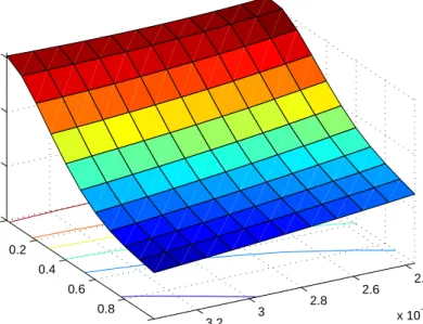
The results when the true model is the one determined by (2) are shown in Figure 1. In both this and the following section,γ andλare linked according to equation (13). The figure shows the ratio
9The lowest value ofλis chosen to ensure thatγ does not exceed unity. 10See Dennis (2010).
2.4 2.6 2.8 3 3.2 x 10 −3 0 0.2 0.4 0.6 0.8 1 0.85 0.9 0.95 1 λy
Relative losses when true model is characterised by indexation
γ
welfare losses
Figure 1: Ratio of losses from the QL policy relative to the optimal policy with perceived rule of thumb pricing.
of losses from the quadratic preferences model to losses under the rule of thumb policy.12
Several results arise. If the ad hoc policy maker sets λy = λx, then losses are always lower under the QL than under the RoT policy for all values of γ except γ = 1, when all models are identical so they possess the same targeting rules. The reason for this is that the true model calls for accommodating inflation persistence, and although the QL policy maker aims to stabilise the level of inflation, there is greater over-reaction under the RoT policy, where persistent inflation is more costly.
As Figure 1 shows, the results are robust to the value ofλy chosen, as long as it is in the vicinity of λx. The crucial parameter is the degree of indexation, and clearly, the RoT policy leads to a
marked reduction in welfare when compared to the QL targeting rule (11).
Given than in this paper the assumption is that the monetary authority can observe the Phillips
12As mentioned above, in the model with indexation to past inflation, losses under the correct policy do not vary
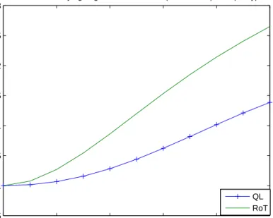
0 0.2 0.4 0.6 0.8 1 0.95 1 1.05 1.1 1.15 1.2 1.25 1.3
Losses for varying degrees of indexation (relative to optimal policy)
γ
Loss
QL RoT
Figure 2: Losses under the QL and RoT policies when true model is indexation, scaled by the optimal targeting rule
curve but not what its structural cause is, it can determine the value ofλx, as it is the same in both
micro-founded models. In this case the QL policy is superior and more robust than that derived from the RoT policy maker. This can be seen in Figure 2, where the losses for each model are shown under the assumption that λx = λy and the results are proportional to losses under the true policy (which is independent of γ). The figure emphasises the fact that whilst using the ad hoc loss function to derive the optimal targeting rule results in misleading policy prescriptions, its performance may be better than the available alternatives.
It still remains to be seen whether the QL targeting rule is also capable of delivering a relatively good performance in other micro-founded models, which will be considered in the next section.
5.2 Inflation persistence as a result of rule of thumb behaviour
Now the true model is characterised by rule of thumb behaviour but again, as the policy maker cannot determine this she may incorrectly infer that the true model is the one where inflation
2.4 2.6 2.8 3 3.2 x 10⁻³ 0.4 0.6 0.8 1 0.2 0.4 0.6 0.8 1 λy
Relative losses when true model is characterised by RoT pricing
λ
welfare losses
Figure 3: Ratio of losses from QL relative to the optimal policy with perceived indexation to past inflation
persistence is caused by indexation. In this context a decrease in λrepresents a higher degree of rule of thumb behaviour and consequently, greater inflation persistence.
The results of using the wrong micro-founded model are even more dramatic than in the previous section. As the degree of RoT rises it becomes increasingly important to stabilise inflation (this is captured by the additional presence of ∆π in the loss function), which is partly fulfilled by the QL policy. But if the policy maker believes that persistence is caused by indexation then it should accommodate it by stabilising the quasi-differenced inflation rate, with disastrous consequences. As the results shown in Figure 3 highlight, the QL policy maker delivers a much better economic performance than the optimal policy under perceived indexation, with the only exception being when there is no rule of thumb behaviour (λ= 1). Similarly to the previous model, allowing the QL policy maker to optimise with a value of λy in the vicinity of λx has only minor effects on the
results.
Both figures 1 and 3, especially the latter one, highlight an important feature of using targeting rules derived from a particular model of pricing behaviour: they can be highly model specific
0.4 0.5 0.6 0.7 0.8 0.9 1 1 1.5 2 2.5 λ
Losses for varying degrees of rule of thumb price setting (relative to optimal policy)
Loss
Indexation QL
Figure 4: Losses under the QL and indexation policies when the true model is RoT. Results are scaled by the losses under the correct policy
and yield conclusions that may be at odds with one another. Higher inflation persistence calls for greater accommodation in one model but greater stabilisation in the other. This calls into question the desirability of following policy prescriptions arising from models that deliver rather specific conclusions. Such a conclusion is most evident when using the policy that results from the indexation model in other contexts. Figure 4 shows the losses under the QL and indexation policies when the true model is RoT, scaled by the losses from the correct policy. The losses resulting from using the ad hoc objective function are dwarfed by those arising with the optimal targeting rule under indexation.
5.3 Expected losses from using the structural loss function
The previous analysis considered the consequences of using the wrong micro-founded loss function and the results clearly highlighted the relatively superior performance of the QL policy. But what is the expected loss of using these models when they may possibly be correct? One can tackle this issue by assuming that both the indexation and RoT models are equally likely. Then the expected
losses of each policy will take into account that the model may in fact be correct. Thus the expected loss function is given by:
EL=χLindt + (1−χ)Lrott (14)
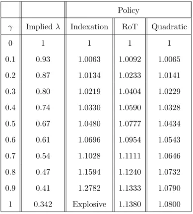
The results can be seen in Table 2 for χ, the probability of the indexation model being true, set to 0.5. The first two columns show the relationship between the values of γ and λacross the two models, indexation and RoT, respectively. The remaining three columns show the losses that are incurred under each policy when both indexation and RoT have a probability of 0.5, with the results scaled by losses when γ = 0 (λ= 1), as in that case both indexation and RoT behaviour revert back to the standard New Keynesian model. For example, the third column (’Indexation’) shows the losses from operating policy (4), but as the true model is unknown, reported losses (again, as mentioned before, scaled) are the average that arise from (3) and (7).
The table highlights the robustness across models of the QL policy. Although the RoT policy is inferior, the indexation policy can result in an explosive solution - and hence infinite losses - in the special case where it is trying to stabilise the differenced inflation rate. Clearly, ad hoc policies are inferior to the true optimal targeting rule when the model is known, but in the presence of observationally equivalent models it does possess the property of robustness that McCallum has so often advocated. These conclusions are rather different from those that obtain when using non-nested models and a common, ad hoc, objective function as in Levin and Williams (2003). There the worst case scenario arises when one uses the optimal policy from a more flexible and forward looking model when the true model exhibits greater rigidities. This is fairly intuitive as such models, being harder to control, require greater and more gradual stabilisation. The reverse is not true; using the policy derived from a more backward-looking model when the economy is in fact forward looking won’t generate an equivalent deterioration in welfare. One can think of this as the stabilising features of such an economy despite the policy maker’s best, but misguided efforts.
Policy
γ Implied λ Indexation RoT Quadratic
0 1 1 1 1 0.1 0.93 1.0063 1.0092 1.0065 0.2 0.87 1.0134 1.0233 1.0141 0.3 0.80 1.0219 1.0404 1.0229 0.4 0.74 1.0330 1.0590 1.0328 0.5 0.67 1.0480 1.0777 1.0434 0.6 0.61 1.0696 1.0954 1.0543 0.7 0.54 1.1028 1.1111 1.0646 0.8 0.47 1.1594 1.1240 1.0732 0.9 0.41 1.2782 1.1333 1.0790 1 0.342 Explosive 1.1380 1.0800
Table 2: Expected losses across both models under alternative policies (normalised to the no infla-tion persistence case). The probability of each model being true is 0.5.
but rather, that when the true model is unknown – or as here – when both models are equally likely, using the quadratic loss function to determine policy may be less misleading than using a micro-founded loss function. Of course, when the probability of one particular model being true is very high this result does not always hold, but it would be hard to argue that of the two models considered in this paper there is a general consensus that one is closer to the true data generating process. The appendix shows the expected losses for two additional value ofχ.
6
Conclusion
Walsh (2005) has criticised the use of exogenously specified policy objectives to analyse monetary policy, especially when assessing the robustness of alternative policy rules. Indeed, much current research has used an approximation to the representative agent’s loss function to derive optimal policies. Any policy that is derived in this manner possesses one key desirable feature: it is consistent with the model being used. Therefore, the use of ad hoc objectives will result in a deterioration in economic performance.
Nevertheless, the use of endogenous objectives will be successful only to the extent that the true model is known. This will be especially the case when alternative models give rise to observationally equivalent Phillips curves, the focus of this paper. Then the issue will be not that objectives are endogenous, but which objectives? Moreover, it may then be the case that the policy derived using exogenous objectives will result on outcomes that are, from the point of view of robustness, superior to those that are optimal in a model that is perceived to be correct by the policy maker. The reason such a result arises is that although micro-founded models may yield the same, or very similar, reduced form equation, the welfare objectives that are consistent with such models can be vastly different.
The analysis of this paper suggests that using ad hock loss functions for policy analysis - where the policy maker’s objective is to minimise a quadratic loss function in inflation and the output gap - whilst not optimal, performs reasonably well when compared to targeting rules derived from
structural, but incorrect, models. Put differently, application of the micro-founded loss function can be even more misleading than the ad hoc objective if the wrong model is being used.
The aim of this paper is not to argue that using the ad hoc loss function is always more robust than using the social loss function from a particular model. Clearly, there may exist models for which this is the case. Rather, the main result is somewhat akin to the popularity of the Taylor rule: it is simple, easy to communicate, and performs reasonably well in a variety of models
Lastly, a further interpretation of the results in this paper is that in the presence of model – and hence objective – uncertainty, it is more robust to assume no inflation persistence when operating under commitment as the resulting objective reverts back to the ad hoc loss function considered here.
References
Adolfson, Malin, Stefan Laseen, Jesper Linde, and Lars E.O. Svensson, “Optimal Mon-etary Policy in an Operational Medium-Sized DSGE Model,” NBER Working Papers 14092, National Bureau of Economic Research, Inc June 2008.
Amato, Jeffery D. and Thomas Laubach, “Rule-of-thumb behaviour and monetary policy,”
European Economic Review, October 2003, 47 (5), 791–831.
Angeloni, Ignazio, Gunter Coenen, and Frank Smets, “Persistence, The Transmission Mech-anism And Robust Monetary Policy,”Scottish Journal of Political Economy, November 2003,50
(5), 527–549.
Benigno, Pierpaolo and Michael Woodford, “Inflation Stabilization And Welfare: The Case Of A Distorted Steady State,” Journal of the European Economic Association, December 2005,
3 (6), 1185–1236.
Bidder, Rhys, Kalin Nikolov, and Tony Yates, “Self-fulfilling inflation persistence,” Technical Report, mimeo 2009.
Casares, Miguel, “A close look at model-dependent monetary policy design,” Federal Reserve
Bank of St. Louis Review, 2006, (Sep), 451–470.
Clarida, Richard, Jordi Gali, and Mark Gertler, “The Science of Monetary Policy: A New Keynesian Perspective,” Journal of Economic Literature, December 1999, 37(4), 1661–1707.
Dennis, Richard, “When is discretion superior to timeless perspective policymaking?,” Journal
of Monetary Economics, April 2010,57(3), 266–277.
Edge, Rochelle M., Thomas Laubach, and John C. Williams, “Welfare-maximizing mon-etary policy under parameter uncertainty,”Journal of Applied Econometrics, 2010,25(1), 129– 143.
Gali, Jordi and Mark Gertler, “Inflation dynamics: A structural econometric analysis,”Journal
of Monetary Economics, October 1999, 44(2), 195–222.
Jensen, Christian and Bennett T. McCallum, “The non-optimality of proposed monetary policy rules under timeless perspective commitment,” Economics Letters, October 2002,77 (2), 163–168.
Levin, Andrew T., Alexei Onatski, John Williams, and Noah M. Williams, “Monetary Policy Under Uncertainty in Micro-Founded Macroeconometric Models,” in “NBER Macroeco-nomics Annual 2005, Volume 20” NBER Chapters, National Bureau of Economic Research, Inc, May 2006, pp. 229–312.
and Jeremy M. Piger, “Is inflation persistence intrinsic in industrial economies?,” Working Paper Series 334, European Central Bank April 2004.
and John C. Williams, “Robust monetary policy with competing reference models,” Journal
of Monetary Economics, July 2003, 50(5), 945–975.
and Richhild Moessner, “Inflation persistence and monetary policy design - an overview,” Working Paper Series 539, European Central Bank November 2005.
McCallum, Bennett T., “Robustness properties of a rule for monetary policy,”
, “Targets, Indicators, and Instruments of Monetary Policy,” NBER Working Papers 3047, Na-tional Bureau of Economic Research, Inc March 1991.
, “Monetary Policy Rules and Financial Stability,” NBER Working Papers 4692, National Bureau of Economic Research, Inc April 1996.
and Edward Nelson, “Timeless perspective vs. discretionary monetary policy in forward-looking models,”Federal Reserve Bank of St. Louis Review, 2004, (Mar), 43–56.
Paez-Farrell, Juan, “Monetary policy rules in theory and in practice: evidence from the UK and the US,” Applied Economics, 2009, 41(16), 2037–2046.
Pivetta, Frederic and Ricardo Reis, “The persistence of inflation in the United States,”Journal
of Economic Dynamics and Control, April 2007,31(4), 1326–1358.
Roberts, John, “How Well Does the New Keynesian Sticky-Price Model Fit the Data?,”
Contri-butions to Macroeconomics, 2005, 5 (1), 1206–1206.
Rotemberg, Julio J. and Michael Woodford, “An Optimization-Based Econometric Frame-work for the Evaluation of Monetary Policy: Expanded Version,” NBER Technical Working Papers 0233, National Bureau of Economic Research, Inc May 1998.
Svensson, Lars E O, “Transparency under Flexible Inflation Targeting: Experiences and Chal-lenges,” CEPR Discussion Papers 7213, C.E.P.R. Discussion Papers March 2009.
Theil, Henri,Economic Forecasts and Policy, Amsterdam: North Holland, 1958.
Tinbergen, Jan,On the Theory of Economic Policy, Amsterdam: Elsevier University Press, 1952.
Walsh, Carl E.,Monetary Theory and Policy, 2nd Edition, Vol. 1 ofMIT Press Books, The MIT Press, January 2003.
, “Endogenous objectives and the evaluation of targeting rules for monetary policy,” Journal of
Monetary Economics, July 2005, 52(5), 889–911.
Woodford, Michael, “Commentary : how should monetary policy be conducted in an era of price stability?,” Proceedings, 1999, pp. 277–316.
, Interest and Prices: Foundations of a Theory of Monetary Policy, Princeton University Press, 2003.
A
Equations underlying the models
A.1 Building blocks
The models used in this paper are variants of the standard New Keynesian framework widely studied in the literature and the details can be found in Woodford (2003), Benigno and Woodford (2005) and Amato and Laubach (2003). The analysis assumes complete markets and that households insure themselves against idiosyncratic risks.
In the absence of an output or employment subsidy, the model is characterised by a distorted steady state. As a result, the flex-price level of output (ynt) will differ from its efficient level,yte, in its response to shocks. The former is given by:
yn
t = [σGt+φ(1 +ν)at−[τ /(1−τ)]τt]/(ω+σ)
Whereas the first-best level of output is described by
ye
t =ω1ynt −ω2Gt+ω3τt
Here, Grepresents government consumption – in log deviation from steady state – andais an aggregate productivity shock. τt denotes an income tax shock, whose steady state value is given
ω1=q−y1[(ω+σ) + Φ(1−σ)] ω2= Φs −1 c σ (ω+σ)2+Φ[(1−σ)(ω+σ)−(s−c1−1)σ] ω3= τ /(1 −τ) (ω+σ)+Φ[(1−σ)−(sc−1−1)σ(ω+σ)−1] with qy ≡ω+σ+ Φ(1−σ)−Φσ(s −1 c −1) ω+σ
The parameter sc represents the steady-state ratio of consumption to output, withσ being the
representative agent’s coefficient of relative risk aversion divided bysc. The elasticity of firm output
with respect to its labour input is given byφ, whilstω=φ(1 +ν)−1 denotes the inverse elasticity of the firm’s marginal cost with respect to its own output. Lastly, Φ measures the inefficiency of steady state output, Y:
Φ = 1−(θ−θ1)(1−τ)
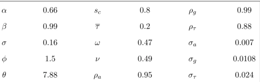
The three shocks, G,aand τ are assumed to be AR processes with values shown in Table 3.
A.2 Structural parameters
The calibration of the structural parameters are chosen to equal those estimated or calibrated by Rotemberg and Woodford (1998) and are shown in Table 3.13 The parameter α, which represents the frequency of price adjustment, is set at 0.66, so that prices are fixed on average for three quarters. The discount factor β is chosen so thatβ−1
−1 equals the long-run average real interest rate, and the value ofθimplies a markup of 15%. Given the latter the value ofφis then calibrated to be consistent with the observed share of labour income in national income. Lastly, ω is equal to
φ(1 +ν)−1, whereν measures the curvature of the disutility of labour function.
Table 3: Structural parameters α 0.66 sc 0.8 ρg 0.99 β 0.99 τ 0.2 ρτ 0.88 σ 0.16 ω 0.47 σa 0.007 φ 1.5 ν 0.49 σg 0.0108 θ 7.88 ρa 0.95 στ 0.024