Optimal Kernel Choice for Domain Adaption Learning
Le Donga,∗, Ning Fenga, Pinjie Quana, Gaipeng Konga, Xiuyuan Chena, Qianni Zhangb
aSchool of Computer Science and Engineering,University of Electronic Science and
Technology of China (UESTC),2006 Xiyuan Avenue, Gaoxin West Zone, Chengdu, Sichuan, 611731, China
bSchool of Electronic Engineering and Computer Science, Queen Mary, University of
London
Abstract
In this paper, a kernel choice method is proposed for domain adaption, referred
to as Optimal Kernel Choice Domain Adaption (OKCDA). It learns a robust
classier and parameters associate with Multiple Kernel Learning side by side.
Domain adaption kernel-based learning strategy has shown outstanding
perfor-mance. It embeds two domains of different distributions, namely, the auxiliary
and the target domains, into Hilbert Space, and exploits the labeled data from the source domain to train a robust kernel-based SVM classier for the target
domain. We reduce the distributions mismatch by setting up a test statistic
between the two domains based on the Maximum Mean Discrepancy (MMD)
algorithm and minimize the Type II error, given an upper bound on error I.
Si-multaneously, we minimize the structural risk functional. In order to highlight
the advantages of the proposed method, we tackle a text classication problem
on 20 Newsgroups dataset and Email Spam dataset. The results demonstrate
that our method exhibits outstanding performance.
Keywords: Optimal Kernel, Domain Adaption, Cross-domain, Test Statistic,
Kernel Choice
∗Corresponding author. Tel.:+86 13981763623; Fax: +86-28-61831655.
1. Introduction
Conventional machine learning methods universally assume that the training
data and the test data come from the same distribution. Unfortunately for many
applications, it is difficult to obtain enough labeled data for training classifiers.
Recently, many researchers have been focusing on cross-domain adaption which
5
aims at solving a learning problem in the target domain by utilizing training
data in the source domain, while these two domains may have different
dis-tributions [1, 2]. In practice, the domain adaptive learning strategy has been successfully applied to real-time applications, such as multi-task clustering [3]
,WiFi localization [4], action recognition [5], sentiment classification [6], visual
10
event recognition [7, 8], object detection [9, 10] and visual concept classification
[11, 12, 13]. However, compared with non-learning methods [14, 15], adaptive
learning has more extensive applications.
To take the advantage of all labeled patterns for both auxiliary and
tar-get domains, Daume [16] proposes a Feature Replication method to augment
15
features for cross-domain learning. The augmented features are then used to
construct a kernel function for Support Vector Machine training. Yang et al.
[12] propose Adaptive SVM for visual concept classification, in which the new classifier fT(x) is adapted from an existing classifier fA(x) trained from the
source domain. Cross-domain SVM proposed by Jiang et al. [11] usesk-nearest
20
neighbors from the target domain to define a weight for each auxiliary pattern,
and then the SVM classifier is trained with the re-weighted auxiliary patterns.
More recently, Jiang et al. [11] proposes a method of mining the relationship
among different visual concepts for video concept detection. They first build a
semantic graph which can be adapted in an online fashion to fit the new
knowl-25
edge mined from the test data. However, these methods do not utilize unlabeled
patterns from the target domain. Such unlabeled patterns can also be used to
improve the classification performance.
When there are only a few or even no labeled patterns available in the target
domain, the auxiliary patterns or the unlabeled target patterns can be used to
train the target classifier. Several cross-domain learning methods are proposed
to cope with the inconsistency of data distributions. These methods re-weighted
the training samples from the source domain by using unlabeled data from the target domain so that the statistics of samples from both domains are matched.
Duan et al. [17, 19] propose a cross-domain kernel learning framework, which
35
learns a kernel function and classifier by minimizing both the structural risk
functional and the distribution mismatch between the labeled and unlabeled
samples from the auxiliary and target domains. This framework employs a
domain similarity measure based on MMD. More recently, Duan et al. [7]
de-velop a cross-domain learning method, referred to as Adaptive Multiple Kernel
40
Learning (A-MKL) that has been successfully used in visual event recognition.
A common insight is that most of those domain adaption learning methods
are either variants of SVM or other kernel methods, which map auxiliary data and target data into a feature space for obtaining a robust SVM-based classifier,
and simultaneously, minimize the mismatch between two different distribution
45
domains. The performance of a classifier strongly depends on the choice of the
kernels. Lanckriet et al. [18] develop a nonparametric kernel matrix, which
involves joint optimization of the coefficients in a conic combination of kernel
matrices. One problem is that its time complexity is too high to be applied to
real applications. In recent years, many effective methods [17, 19, 20, 21, 22]have
50
been developed to combine multiple kernels instead of directly learning the
kernel matrix, in which the kernel function is a linear combination of based
kernel functions. However, all those methods suppose that both test and training data are drawn from the same distribution. Consequently, naked multiple kernel
learning cannot directly solve the problem of cross-domain learning. Because
55
the coefficients of combination kernel are parameterized, the training data from
source domain may degrade the performance of the model in the target domain.
In this paper, we propose a new method on kernel choice for cross-domain
learning, which explicitly minimizes the loss due to the bias between the data
distributions of the auxiliary and target domains, as well as the cost function
60
wrongly rejecting null hypothesis when the auxiliary distribution and the target
distribution are drawn from the same distribution. Type II error is the
prob-ability of wrongly accepting null hypothesis when the auxiliary and the target distributions are different. Given an upper bound on Type I error, our kernel
65
choice minimizes Type II error. The main contribution of this paper is that
multiple base kernels are weighted to minimize the loss on the labeled examples
and the bias between the data distributions in the two domains. Meanwhile, we
minimize the bias between the source domain and the target domain by
mini-mizing the Type II error. While multi-kernel method has been widely discussed
70
[23, 24, 20] and used [21], our work demonstrates that the kernel choice is pivotal
to cross-domain learning.
The rest of paper is organized as follows: We briefly review the related
works in Section 2. Section 3 introduces kernel choice for domain adaption learning. We experimentally compare the proposed method with other
cross-75
domain learning methods on the 20 Newsgroups dataset and Email Spam dataset
for text classification in Section 4. Finally, conclusion is made in Section 5.
2. Brief Review of Related Work
Let us denote the dataset of labeled and unlabeled patterns from the target
domain asDT l = (x T i , yTi )| nl i=1andD T u = (xTi, yiT)| nl+nu i=nl+1, respectively, wherey T i 80 is the label ofxT
i , labeled patterns are numbered 1 tonl, unlabeled patterns are
numberednl+ 1 tonl+nu. We defineDT =DTl
SDT
u as the dataset from the
target domain with the sizent=nl+nu under the marginal data distribution
ρ, and DA = (xA i, yiA)|
nA
i=1 as the dataset from the source domain under the marginal data distribution ϑ. We represent the labeled training dataset as
85
D= (xi, yi)|ni=1, where n is the total number of labeled patterns. The labeled training data can be from the target domain(D =DTl ) or from both domains
(D=DTl S DA).
2.1. Minimize Bias of Distribution Using Test Statistic
It is important to reduce the mismatch between the source domain and the
target domain distributions, and many methods have been proposed to address
this work. A classic criteria is Kullback Leibler divergence[25]. However, most
of them are parametric and need to estimate an intermediate density. To steer
clear of fussy measure, Borgwardt et al. [26] present a novel non-parametric
statistical method, namely, Maximum Mean Discrepancy, which is based on
Reproducing Kernel Hilbert Space [27].
M M D(DA, DT) = sup kfkH≤1 (ExA∼Q[f(xA)]−ExT∼P[f(xT)]) = sup kfkH≤1 hf,(ExA∼Q[f(xA)]−ExT∼P[f(xT)]) =kExA∼Q[f(xA)]−ExT∼P[f(xT)]kH, (1)
whereEx∼µ[·] denotes the expectation operator under the samples distribution
µandf(x) is any function inH. The second equality holds asf(x) =hf, φ(x)iH
by the property of RKHS, whereφ(x) is the nonlinear feature mapping of the
kernelk. Note that the inner product of φ(xi) andφ(xj) equals to the kernel
functionk(·,·) onxi and xj, namely,k(xi, xj) =φ(xi)φ(xj). An expression for
the squared MMD is
ηk(DA, DT) =kφ(DA)−φ(DT)k2H (2)
=Exx0k(x, x0) +Eyy0k(y, y0)−2Eyx0k(y, x0), (3)
wherex, x0 ∼i.i.dpandy, y0 ∼i.i.dq. By introducingh
k(x, x0, y, y0) =k(x, x0) + 90
k(y, y0)−k(y, x0)−k(x, y0), Eq.(2) can be rewritten asηk=Exx0yy0hk(x, x0, y, y0).
By introducing hk(x, x0, y, y0) = k(x, x0) +k(y, y0)−k(y, x0)−k(x, y0), Eq.(2)
can be rewritten asηk=Exx0yy0hk(x, x0, y, y0). In brief, the key point of MMD
is that the distance between distributions of two domains is equivalent to the
distance between the means of the two domains mapped into a RKHS [4]. Huang
95
et al. [28] develop a two-step method. The first step is to diminish the mismatch of means of different distributions in RKHS by reweighting the examples using
square MMD. The seconed step is to learn a decision function that separates
patterns from two opposite classes. One difficulty is that the performance of
MMD strongly depends on the choice of kernel. Meanwhile, these methods do
100
not ensure that the chosen kernel is optimal. Inspired by [29], we review the
problem of bias between the source domain and the target domain as a
two-sample test problem, which addresses the question of whether two independent
samples are drawn from the same distribution. Consequently, given two example
distributions: q from source (auxiliary) domain and pfrom target domain, we
105
can set up a two-sample test which measures the similarity or bias between the
source domain and the target domain.
We select some kernels for hypothesis testing from a particular familyK of
kernels, assuming kernelk(xi, xj) is a linear combination of a set of base kernels
kd=
M
X
m=1
dmkm, (4)
wheredm>0 is a set of positive coefficients , M P m=1 dm=D >0. The squared MMD becomes ηm(DA, DT) =kφ(DA)−φ(DA)k2z= M X l=1 dlηl(DA, DT). (5)
Here, it is denoted thatd={d1, d2, . . . , dM}T ∈RM×1, η ={η1, η2, . . . , ηM} ∈
RM×1. Eq.(5) can be written as η
m(DA, DT) = dTη. ηm is the average of
independent random variables, and its asymptotic distribution is given by the
central limit theorem. Now we set up the construction of a hypothesis test and
define Φ as the Cumulative Distribution Function (CDF) of a standard normal
random variableN(0,1) , where Φ−1 is the inverse CDF. A test of asymptotic
level α using the statistics will have a threshold t as in [14]. To obtain an
estimate of the variance based on the samples, we use an expression derived
from the U-statistic. The population variance can be written as
σ2=Exx0yy0h2k(x, x0, y, y0)−[Exx0yy0hk(x, x0, y, y0)]2. (6)
The choice of kernel will affect both the test statistic and the asymptotic
t. The asymptotic probability of a Type II error is therefore expressed as:
P(ηm< t) = Φ(Φ−1(1−ϑ)−ηk(DA, DT)
√
n /√2σk), (7)
where Φ is a monotonic function, n is the number of all patters and t is the
threshold of the test statistic and is set to√2n−1/2σ
kΦ−1(1−ϑ). Obviously,
the Type II probability will decrease as the ratioηm(DA, DT)σk−1 increases. 110
2.2. Borrow Knowledge From Ready-Made Classifier
Instead of directly utilizing the source domain data to learn a classifier,
many researchers consider learning a final classifier from a pre-learned classifier
trained by an source domain [17]. Yang et al. [12] develop Adaptive SVM, in
which a new SVM classifier is adapted from a pre-learned auxiliary classifier
115
trained with patterns from the source domain. Schweikert et al. [30] propose to
use linear combination of the decision values from an auxiliary SVM classifier
and the target SVM classifier for prediction in the target domain. Besides, Jiang
et al. [13] propose a new cross-domain SVM (CDSVM) algorithm for adapting
previously learned support vectors from the source domain to help classification
120
in another domain. Whereas, it should be noted that all of them do not make use of unlabeled data in the target domain for cross learning. Duan et al. [17]
utilize the unlabeled data in the target domain. The problem is how to minimize
the mismatch of two distribution by MMD, which do not utilize the chance to
select an optimal kernel for the classifier. Recently, some unsupervised kernel
125
learning methods [31, 32] are proposed. Pan et al. [4] demonstrate a Maximum
Mean Discrepancy Embedding, which minimizes the square of the Maximum
Mean Discrepancy criterion, and then applies the learned kernel matrix to train
SVM classifier for WiFi localization and text categorization. Different from
these approaches, we propose a kernel choice method for domain adaption, they
130
are better in extending the previous work on optimal kernel choice to two-sample tests. The proposed approaches are described in full details in section 3.
3. Optimal Kernel Choice for Domain Adaption Learning
Similar to previous methods, we assume the kernel function is a linear
com-bination of a set of base kernels. Our goal is to learn a function of the form
f(x) =wø(x) +bwith multiple kernels k(xi, xj) = d
P
i=1
βik(xi, xj) representing
the inner product in a feature space parameterized by β. At the same time,
we minimize the bias of different distributions between the source domain and
the target domain. The definition of an object function for domain adaption
learning can be formulated as
arg min d∈D Φ(P(ηk < t)) +λΥ(d), (8) where Υ(d) = min w,ξ,b kwk 2/2 +C l X i=1 ξi+ Ω(d) (9) s.t. 1−ξi≤yi( n X i wiφ(xi) +b), 0≥ξ, 0≤d. where φ(xi)φ(xj) = M X i=1 diφi(xi)φi(xj) (10)
Note that Φ(·) is a monotonic increasing function, and Ω(d) is constraint func-tion withd. nis the total number of training samples. Υ(d) is the regularizer
function and can be any differentiable function ofdwith continuous dervative.
λis a tradeoff parameter. C>0 is regularization parameter where the objective
term is near to the standardC-SVM objective term. Given the misclassification
C, the aim is to maximise the margin while minimizing the hinge loss on the labeled data between the auxiliary and the target domains. The only addition
is an regularisation on the weightsd associated with multiple kernels. Recall
in [29] it is shown that minimizing the Type II error, P(ηk < t), is equal to
minimizingd0Qd, whereQis the covariance matrixcov(h). The models [29] are
referred to full details. Let us define
then, the optimization problem can be rewritten as min d∈DT(d) = minw,b,ξ J(d) +λ(w 0w/2 +C l X i=1 ξi) (12) s.t. 1−ξi≤yi( d X i wiø(xi) +b) 0≤ξ, 0≤d.
However, the objective function term in the brackets and the constraints are
the standardC-SVM object. λis set to 0.1, 0.2, 0.5, 1, 2, 5, 10, 20, 50. It is
straightforward to derive the corresponding dual problem
W(d) = max
α 1
T
α−1/2αTdα+J(d)
1TY α= 0, 0≤α≤C, (13)
where Kd is the kernel matrix for a given d, Y is a diagonal matrix with the
labels on the diagonal. In this paper, we utilize project gradient descent in the outer loop to obtaind. According to [22],W can be differentiated with respect
todas ifα∗ does not depend ond. We therefore get
∂T /∂d=∂W /∂d=∂J /∂d−α∗TY(∂Kd/∂d)Y α∗/2
∂2T /∂d2=∂2W /∂d2=∂2J /∂d2. (14)
In our learning method, we employ the reduced gradient descent procedure
proposed by iteratively updating the linear combination coefficient d and the
135
dual variableα. There are two stages in this process:
The first stage: d is fixed, thus Ω(d) is a constant. We solve Eq.(14) to obtain the dual variableα.
The second stage: Based on the first stage,αis fixed. Use the projected gradient descent process method to obtain d. With respect tod, the objective
functionM(d) can be rewritten as
We adopt the second-order gradient descent method to update the linear
com-bination coefficientdat iterationk+ 1 by
dk+1=dk−εk∇2G, (16)
where εt is the learning rate which can be computed by using a line search
method, in which∇2Gis the updating direction. It is worthwhile to note that
140
Q is not a full rank. To avoid numerical instability, we define Q = Q+ςE, whereς is set to 10−6 in the experiment.
4. Experiment
In this section, we’ll evaluate the effectiveness of our approach. We
com-pare our kernel choice approach for domain adaption, with the baseline SVM,
145
and some state-of-the-art domain adaptation learning methods, such as
Fea-ture Replication [16], Adaptive SVM (A-SVM) [12], CDSVM [13], MKL and
DMKLDF [17]. In our experiment, we focus on challenging text classification
problems on 20 Newsgroups dataset1and Email Spam dataset.
4.1. Datasets Description
150
The 20 Newsgroups dataset is a collection of approximately 20 000
news-group documents, partitioned (nearly) evenly across six main categories and 20
different newsgroups, each corresponding to a different topic. Some of the
news-groups are very closely related to each other (e.g. comp.sys.ibm.pc.hardware
vs. comp.sys.mac.hardware), while some others are highly unrelated (e.g
mis-155
c.forsale vs. soc.religion.christian). The 20 newsgroups collection is a popular
dataset for experiments in text applications of machine learning techniques.
In our experiment, we follow experiment setting of [7]. The four largest main
categories are chosen for evaluation. Specifically, for each main category, the
largest subcategory is selected as the target domain, while the second largest
160
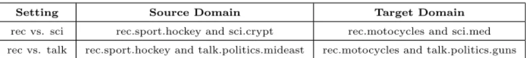
subcategory is chosen as the source domain. Table 1 provides the detailed
Setting Source Domain Target Domain
rec vs. sci rec.sport.hockey and sci.crypt rec.motocycles and sci.med rec vs. talk rec.sport.hockey and talk.politics.mideast rec.motocycles and talk.politics.guns
Table 1: Description of 20 Newsgroups Dataset
information of selected two settings. To build the training dataset, we also use
all labeled samples from the source domain, and at the same time randomly
choose m positive and m negative samples from the target domain. In the
experiment, m is set to 0, 1, 3, 5, 7 and 10. There are three email subsets
165
(denoted by User1, User2, and User3, respectively) annotated by three different
users in the email spam dataset. The task is to classify spam and non-spam
emails.
Setting Source Domain Target Domain
User0 vs. User1 User0 User1
User1 vs. User2 User1 User2
User2 vs. User0 User2 User0
Table 2: Description of Email Spam Dataset
Since the spam and non-spam emails in the subsets have been differentiated
by different users, the data distributions of the three subsets are related but
170
different. Each subset has 2 500 emails, in which half of the emails are
non-spam (labeled as 1) and the other half of them are non-spam (labeled as -1). In
this dataset, we consider three settings as in Table 2. For each setting, the
training dataset contains all labeled samples from the source domain as well
as the labeled samples from the target domain, in which five positive and five
175
negative samples are randomly chosen, and the remaining samples in the target domain are used as unlabeled training data and test data as well. We randomly
sample the training data from the target domain for five times and report the
means and the standard deviations of all methods. Again, the word-frequency
feature is used to represent each document.
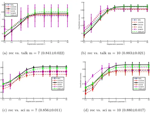
0.1 0.2 0.5 1 2 5 10 20 50 0.65 0.7 0.75 0.8 0.85 0.9 Regularization parameter C Classification accuracy MKL CDSVM OKCDA ASVM SVMFR DMKLDF
(a) rec vs. talk m = 7 (0.841±0.022)
0.1 0.2 0.5 1 2 5 10 20 50 0.65 0.7 0.75 0.8 0.85 0.9 Regularization parameter C Classification accuracy MKL CDSVM OKCDA ASVM SVMFR DMKLDF (b) rec vs. talk m = 10 (0.883±0.021) 0.1 0.2 0.5 1 2 5 10 20 50 0.6 0.65 0.7 0.75 0.8 0.85 Regularization parameter C Classification accuracy MKL CDSVM OKCDA ASVM SVMFR DMKLDF (c) rec vs. sci m = 7 (0.856±0.011) 0.1 0.2 0.5 1 2 5 10 20 50 0.65 0.7 0.75 0.8 0.85 0.9 Regularization parameter C Classification accuracy MKL CDSVM OCKDA ASVM SVMFR DMKLDF (d) rec vs. sci m = 10 (0.880±0.017) Figure 1: Performance comparisons of OKCDA with other methods in terms of the means and standard deviations of classification accuracies on the 20 Newsgroups dataset with different regularization parametersC∈ {0.1,0.2,0.5,1,2,5,10,20,50}. We setm= 7 orm= 10.
4.2. Experiment Setup
Our base kernels are predetermined for all methods. Specifically, the
follow-ing kernels have been used: Gaussian kernel(i.e.,k(xi, xj) = exp(−γkxi−xjk)),
Linear kernel (i.e., k(xi, xj) =xi·xj) and Polynomial kernel (i.e.,k(xi, xj) =
(xi·xj+1)γ), where the kernel parameterγis set as the default value 0.0005. We 185
use 10 kernel parameters 1.5ξ+1γ, ξ∈ {−2.5,−2,· · ·,2,2.5}. Motivated by [33], the regularization term ofJ(d) is used, which is differentiable and continuous. l1 regularization withJ(d) =dor variations could be used for learning sparse solutions. Alternatively,l2regularization of the formJ(d) = (d−µ)0Σ−1(d−µ) can be used only when a small number of relevant kernels are present or if prior
190
knowledge in the formµand Σ is available.
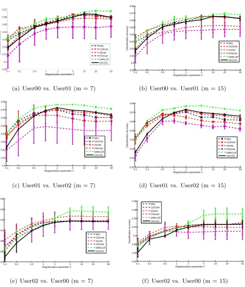
(a) User00 vs. User01 (m = 7) 0.1 0.2 0.5 1 2 5 10 20 50 0.89 0.9 0.91 0.92 0.93 0.94 0.95 0.96 0.97 0.98 Regularization parameter C Classification accuracy MKL CDSVM ASVM FRSVM DMKLDF OKCDA (b) User00 vs. User01 (m = 15) 0.1 0.2 0.5 1 2 5 10 20 50 0.9 0.91 0.92 0.93 0.94 0.95 0.96 0.97 0.98 Regularization parameter C Classification accuracy MKL CDSVM ASVM FRSVM DMKLDF OKCDA (c) User01 vs. User02 (m = 7) 0.1 0.2 0.5 1 2 5 10 20 50 0.91 0.92 0.93 0.94 0.95 0.96 0.97 0.98 Regularization parameter C Classification accuracy MKL CDSVM ASVM FRSVM DMKLDF OKCDA (d) User01 vs. User02 (m = 15) 0.1 0.2 0.5 1 2 5 10 20 50 0.84 0.86 0.88 0.9 0.92 0.94 0.96 Regularization parameter C Classification accuracy MKL CDSVM ASVM FRSVM DMKLDF OKCDA
(e) User02 vs. User00 (m = 7)
0.1 0.2 0.5 1 2 5 10 20 50 0.84 0.86 0.88 0.9 0.92 0.94 0.96 0.98 Regularization parameter C Classification accuracy MKL CDSVM ASVM FRSVM DMKLDF OKCDA (f) User02 vs. User00 (m = 15) Figure 2: Performance comparisons of OKCDA with other methods in terms of the means and standard deviations of classification accuracies on the Email Spam dataset with different regularization parametersC∈ {0.1,0.2,0.5,1,2,5,10,20,50}. We setm= 7 orm= 10.
which has been used as the official performance metric in TRECVID since 2001.
AP is related to multipoint Average Precision value of a precision-recall curve
and incorporates the effect of recall when it is computed over the entire
classi-195
fication results [34]. Thanks to previous work [7], some Matlab code has been
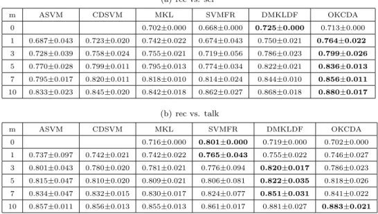
referenced for this purpose in our experiment. Table 3 shows the classification
accuracies and standard deviations of classification accuracies of different
meth-ods on the real dataset. We obtain that the performance of our model improves
obviously with the increasing of m, and achieves the best result when m is set
200
to 10.
Table 4 presents the best among all the results obtained by using different
regularization parametersC∈ {0.1,0.2,0.5,1,2,5,10,50}.
4.3. Results of 20 Newsgroups Dataset
In our experiment, we also compare our proposed method with the
com-205
petitive methods on the classification performance, including MKL, ASVM,
CDSVM, SVMFR and DMKLDF. Different regularization parameters are used.
Fig. 1 shows the variation in classification accuracies with varying C over a
range [0.1, 0.2, 0.5,1, 2, 5, 10, 50]. Note that the x-axis in Fig. 1 are in logarith-mic scale. The results of all methods are obtained by using m positive and m
210
negative training samples from the target domain, as well as the training data
from the source domain, where m = 7 and 10 for the 20 Newsgroups dataset.
We have the following observations:
From the Fig. 1, we observe that when C becomes larger, all methods tend
to have better performance. However, our method OKCDA outperforms most
215
other methods, only except DMKLDF in terms of mean classification accuracies.
Fig. 1(a) shows that SVMFR has the largest standard deviations of classification
accuracies.
• We observe from Fig. 1(b), Fig. 1(c) and Fig. 1(d) that standard deviations of classification accuracies of SVMFR severely changes as C from 0.1 to
220
(a) rec vs. sci m ASVM CDSVM MKL SVMFR DMKLDF OKCDA 0 0.702±0.000 0.668±0.000 0.725±0.000 0.713±0.000 1 0.687±0.043 0.723±0.020 0.742±0.022 0.674±0.043 0.750±0.021 0.764±0.022 3 0.728±0.039 0.758±0.024 0.755±0.021 0.719±0.056 0.786±0.023 0.799±0.026 5 0.770±0.028 0.799±0.011 0.795±0.013 0.774±0.034 0.822±0.021 0.836±0.013 7 0.795±0.017 0.820±0.011 0.818±0.010 0.814±0.024 0.844±0.010 0.856±0.011 10 0.833±0.023 0.845±0.020 0.842±0.018 0.862±0.027 0.868±0.018 0.880±0.017 (b) rec vs. talk m ASVM CDSVM MKL SVMFR DMKLDF OKCDA 0 0.716±0.000 0.801±0.000 0.719±0.000 0.702±0.000 1 0.737±0.097 0.742±0.021 0.742±0.022 0.765±0.043 0.755±0.022 0.746±0.027 3 0.801±0.043 0.780±0.020 0.781±0.021 0.776±0.094 0.820±0.017 0.786±0.023 5 0.815±0.047 0.810±0.020 0.809±0.021 0.806±0.081 0.822±0.035 0.818±0.026 7 0.834±0.047 0.832±0.015 0.830±0.017 0.824±0.077 0.851±0.031 0.841±0.022 10 0.857±0.011 0.856±0.013 0.855±0.013 0.861±0.017 0.881±0.027 0.883±0.021
Table 3: Mean and Standard Deviation (in Percentages) of Classification Accuracies for All Methods with Different Number of Positive and Negative Training Samples from the Target Domain on the 20 Newsgroups dataset. The best results are marked with bold.
all methods is represented linearly ranged from 0 to 2, while it becomes
steady when C is greater than 2. C=2 seems to be a turning point. The
result shows that the classification accuracy does not depend strongly on
the value of regularization parameterCand the existence of a stable value
225
of C. It is interesting to note that our proposed method slightly
under-performs others in terms of classification accuracy asCranged from 0.1 to
2, but it outperforms the other methods in most cases whenC is greater than 2.
To take a deeper look at Table 3, we analyse the performance of our method
230
in comparison with other methods.
• In Fig 2(a), We observe that ASVM performs poorly for all cases. This may be attributed to the distribution difference between the source domain
and the target domain. Whenmis set to 0, the performance of our method
is not better than other methods, because the unlabeled patterns are not
0.1 0.2 0.5 1 2 5 10 20 50 0.95 0.952 0.954 0.956 0.958 0.96 0.962 0.964 0.966 0.968 0.97 parameter lambda classification accuracy C = 1 C = 7 C = 15
(a) User00 vs. User01
0.1 0.2 0.5 1 2 5 10 20 50 0.94 0.945 0.95 0.955 0.96 0.965 parameter lambda Classification accuracy C = 1 C = 15 C =7 (b) User01 vs. User02
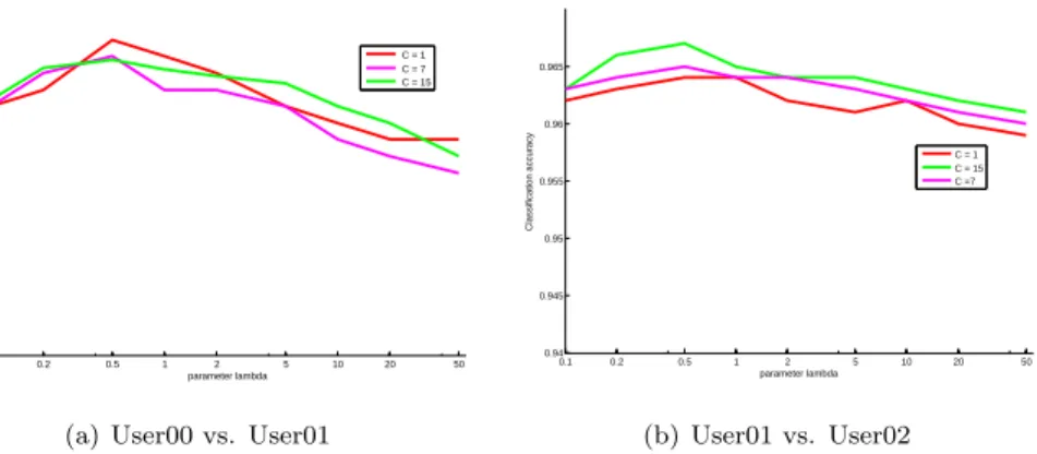
Figure 3: Performance (i.e, the means of classification accuracies) of OKCDA on the Email Spam dataset with different balance parameterλ∈ {0.1,0.2,0.5,1,2,5,10,20,50}, and we set m= 15.
utilized in this case. Note that when m is greater than 0, our proposed
method is consistently better than all other methods in terms of mean
classification accuracies. As m becomes larger, the advantage becomes
more evident.
• In Fig 2(b), we observe that SVMFR have outperforms all other methods
240
when m is set to 0, which is unexpected. We can see DMKLDF have a
stable performance in most cases. Our proposed method outperforms all
other case when m is set to 10. From Table 2(a) and Table 2(b), we have
the following conclusions: many cross-domain learning methods generally
achieve similar performances, and our proposed kernel choice method for
245
cross-domain learning is better than most other methods in terms of the
means of classification accuracies on datasets.
4.4. Results of Email Spam Dataset
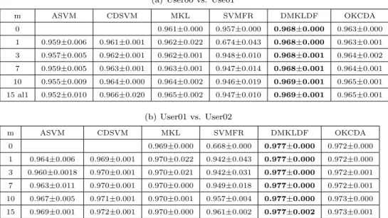
For the Email Spam classification task, we also provide comparisons between
OKCDA and other related methods. For each setting, we report the results of
250
all methods by using the training data from the source domain as well as m
positive and m negative training samples randomly selected from the target
training data from the target domain for five times. In Table 4, we report the
means and standard deviations of classification accuracies for all methods on
255
the Email Spam datasets, respectively. Also noted that for all methods, each result in Table 4 is the best among all the result obtained by using different
regularization parametersC∈ {0.1,0.2,0.5,1,2,5,10,20,50}. From Table 4, we have the following observations:
• The performance of these methods has not been changed greatly under the
260
change of parameter m. OKCDA and DMKLDF have the similar results
and smallest standard deviation of both are significantly less than other
methods. This fact demonstrates that OKCDA and DMKLDF have a
relatively high stability.
• The experimental performance of our method is better than CDSVM,
265
MKL and SVMFR. Compared with DMKLDF, our method has an
ap-proximate performance, which achieves a gap of 0.001 level.
• Since the change of m has not improved the performance of these methods, we believe that there exists a limit among these cross-domain learning
methods. In other words, when the number of samples exceeds a certain
270
threshold, further increasing the training set size does not improve the
performance.
• Our proposed method OKCDA consistently performs better than some methods in terms of the means classification accuracies on Email Spam
dataset, thanks to the explicit modeling of the data distribution mismatch,
275
as well as the successful utilization of the unlabeled data. As shown in
Table 4, when the number of labeled positive and negative training samples
from the target domain increases, OKCDA has similar performance with
DMKLDF but the performance does not improve.
We also compare our proposed method OKCDA with other cross-domain
280
learning methods , including ASVM, CDSVM ,SVMFR and DMKLDF, by
(a) User00 vs. Use01 m ASVM CDSVM MKL SVMFR DMKLDF OKCDA 0 0.961±0.000 0.957±0.000 0.968±0.000 0.963±0.000 1 0.959±0.006 0.961±0.001 0.962±0.022 0.674±0.043 0.968±0.000 0.963±0.001 3 0.957±0.005 0.962±0.001 0.962±0.001 0.948±0.010 0.968±0.001 0.964±0.002 7 0.959±0.005 0.963±0.001 0.963±0.001 0.947±0.014 0.968±0.001 0.964±0.001 10 0.955±0.009 0.964±0.000 0.964±0.002 0.946±0.019 0.969±0.001 0.965±0.001 15 al1 0.952±0.010 0.966±0.020 0.965±0.002 0.947±0.010 0.969±0.001 0.965±0.001 (b) User01 vs. User02 m ASVM CDSVM MKL SVMFR DMKLDF OKCDA 0 0.969±0.000 0.668±0.000 0.977±0.000 0.972±0.000 1 0.964±0.006 0.969±0.001 0.970±0.022 0.942±0.043 0.977±0.000 0.972±0.000 3 0.960±0.0018 0.970±0.001 0.970±0.021 0.942±0.031 0.977±0.000 0.972±0.001 7 0.963±0.011 0.970±0.001 0.970±0.000 0.949±0.018 0.977±0.000 0.972±0.001 10 0.967±0.005 0.971±0.001 0.970±0.001 0.957±0.004 0.977±0.000 0.973±0.000 15 0.969±0.001 0.972±0.001 0.970±0.000 0.961±0.002 0.977±0.002 0.973±0.001
Table 4: Mean and Standard Deviation (in Percentages) of Classification Accuracies for All Methods with Different Number of Positive and Negative Training Samples from the Target Domain on the Email Spam dataset. The best results are marked with bold.
result of all methods are also obtained by using m positive and m negative
training sample from the target domain as well as the training samples from the
source domain. We setm= 7 and m= 15 for Email Spam datasets in Fig. 2.
285
From the Fig. 2, we observe that whenC becomes larger, all methods tend to
have better performances. However, OKCDA has relatively stable performance
in terms of the standard deviations of classification accuracies.
4.5. An analysis of theλtradeoff between the structural risk and the bias min-imization
290
In this subsection, we mainly investigate how would the choice ofλaffect the
adaptation classification accuracy. Fig. 3 shows the variation in classification
accuracies with varying λ of [0.1, 0.2, 0.5, 1, 2, 5, 10, 20, 50], where we set
m=15 and the regularization parameter C =1,7 and 15. Noted that the number
of labeled samples from the two domains and the number of unlabeled samples
295
x-axis in Fig. 3 are in logarithmic scale. We have the following observations:
• The performance of OKCDA changes with differentλvalues. λis a hyper-parameter that the model is not sensitive to, and needs to be tuned across
different labeled or unlabeled data sizes.
300
• Whenλranges from 0.1 to 50, the classification accuracy changes with a small scale. When theλis gradually increasing, the performance decreases
a bit.
• Whenλtakes the value around 5, the best performance of OKCDA can be obtained. In this case, both the labeled data and the unlabeled data from
305
the target domain can be effectively utilized to learn a robust classifier.
5. Conclusions
In this paper, we propose a method of optimal kernel choice for domain
adaption, namely, OKCDA. The paper extends the previous work on optimal
kernel choice to two-sample tests, with an additional component to minimize the
310
structural risk on the labeled data. The method is tested on the 20 Newsgroups
dataset and Email Spam dataset, and compared to several existing methods. In
our experiments, the kernel is set to be a linear combination of some base kernels.
The kernel parameters are chosen to minimize the structural risk functional
and the distribution bias between the samples from the auxiliary and target
315
domains. To reduce the distribution mismatch, we minimize the Type II error based on the MMD and construct a test statistic between source domain and
target domain. We will investigate how to choose the kernel automatically and
explore the relationship between Type II error or Type I error and domain
adaption learning performance in the future.
320
Acknowledgments
This work was supported in part by the National Natural Science Foundation
for the Central Universities (No. ZYGX2013J083), and in part by the
Scien-tific Research Foundation for the Returned Overseas Chinese Scholars, State
325
Education Ministry.
6. References
[1] S. Zhong, X. Zeng, S. Wu, L. Han, Sensitivity-based adaptive learning rules
for binary feedforward neural networks, IEEE Trans. Neural Networks and
Learning Systems. 23 (3) (2012) 480–491.
330
[2] S. J. Pan, I. W. Tsang, J. T. Kwok, Q. Yang, Domain adaptation via
transfer component analysis, IEEE Trans. Neural Networks. 22 (2) (2011)
199–210.
[3] Z. Zhang, J. Zhou, Multi-task clustering via domain adaptation, Pattern
Recognition. 45 (1) (2012) 465–473.
335
[4] S. J. Pan, J. T. Kwok, Q. Yang, Transfer learning via dimensionality
reduc-tion, in: Association for the Advancement of Artificial Intelligence, Vol. 8,
2008, pp. 677–682.
[5] X. Wu, D. Xu, L. Duan, J. Luo, Action recognition using context and
appearance distribution features, in: IEEE 2011 Conference on Computer
340
Vision and Pattern Recognition, 2011, pp. 489–496.
[6] J. Blitzer, M. Dredze, F. Pereira, Biographies, bollywood, boom-boxes and
blenders: Domain adaptation for sentiment classification, in: Annual
Meet-ing of the Association for Computational LMeet-inguistics, Vol. 7, 2007, pp. 440–
447.
345
[7] L. Duan, D. Xu, I. H. Tsang, J. Luo, Visual event recognition in videos
by learning from web data, IEEE Trans. Pattern Analysis and Machine Intelligence. 34 (9) (2012) 1667–1680.
[8] D. Xu, S. F. Chang, Video event recognition using kernel methods with
multilevel temporal alignment, IEEE Trans. Pattern Analysis and Machine
350
Intelligence. 30 (11) (2008) 1985–1997.
[9] D. Vzquez, A. M. Lpez, D. Ponsas, Virtual worlds and active learning for human detection, in: Proceedings of the 13th international conference on
multimodal interfaces, 2011, pp. 393–400.
[10] D. Vzquez, A. Lpez, D. Ponsa, J. Marin, Cool world: domain adaptation
355
of virtual and real worlds for human detection using active learning, in:
Advances in Neural Information Processing Systems-Workshop on Domain,
2014.
[11] Y.-G. Jiang, J. Wang, S.-F. Chang, C. W. Ngo, Domain adaptive semantic
diffusion for large scale context-based video annotation, in: IEEE 12th
360
International Conference on Computer Vision, 2009, pp. 1420–1427.
[12] J. Yang, R. Yan, A. G. Hauptmann, Cross-domain video concept detection
using adaptive svms, in: Proceedings of the 15th international conference
on Multimedia, 2007, pp. 188–197.
[13] W. Jiang, E. Zavesky, S. F. Chang, A. Loui, Cross-domain learning methods
365
for high-level visual concept classification, in: IEEE 15th International
Conference on Image Processing, 2008, pp. 161–164.
[14] L. Dong, J. Su, E. Izquierdo, Scene-oriented hierarchical classification of
blurry and noisy images, IEEE Trans. Image Processing. 21 (5) (2012)
2534–2545.
370
[15] L. Dong, E. Izquierdo, A topology synthesizing approach for classification
of visual information, in: CBMI 2008 International Workshop on
Content-Based Multimedia Indexing, 2008, pp. 373–380.
[16] H. Daume III, Frustratingly easy domain adaptation, in: Proceedings of
the 45th Annual Meeting of the Association of Computational Linguistics,
375
[17] L. Duan, I. W. Tsang, D. Xu, Domain transfer multiple kernel learning,
IEEE Trans. Pattern Analysis and Machine Intelligence. 34 (3) (2012) 465–
479.
[18] G. R. Lanckriet, N. Cristianini, P. Bartlett, L. E. Ghaoui, M. I. Jordan,
380
Learning the kernel matrix with semidefinite programming, The Journal of
Machine Learning Research. 5 (2004) 27–72.
[19] L. Duan, D. Xu, I. W. Tsang, Domain adaptation from multiple sources: A
domain-dependent regularization approach, IEEE Trans. Neural Networks
and Learning Systems. 23 (3) (2012) 504–518.
385
[20] Y. Lu, L. Wang, J. Lu, J. Yang, C. Shen, Multiple kernel clustering based
on centered kernel alignment, Pattern Recognition. 47 (11) (2014) 3656–
3664.
[21] A. Salah, H. M. Mohammand, Z. Xiao, M. V. Richard, Human
activi-ty recognition using multi-features and multiple kernel learning, Pattern
390
Recognition. 47 (5) (2014) 1800–1812.
[22] M. Varma, B. R. Babu, More generality in efficient multiple kernel learning,
in: Proceedings of the 26th Annual International Conference on Machine
Learning, 2009, pp. 1065–1072.
[23] J. Bootkrajang, A. Kab´an, Learning kernel logistic regression in the
pres-395
ence of class label noise, Pattern Recognition. 47 (11) (2014) 3641–3655.
[24] H. Jia, Y. M. Cheung, J. Liu, Cooperative and penalized competitive
learn-ing with application to kernel-based clusterlearn-ing, Pattern Recognition. 47 (9)
(2014) 3060–3069.
[25] Z. Rached, F. Alajaji, L. Campbell, The kullback-leibler divergence rate
400
between markov sources, IEEE Trans. on Information Theory. 50 (5) (2004)
[26] K. M. Borgwardt, A. Gretton, M. J. Rasch, H. P. Kriegel, B. Sch¨olkopf,
A. J. Smola, Integrating structured biological data by kernel maximum
mean discrepancy, Bioinformatics. 22 (14) (2006) e49–e57.
405
[27] R. Rosipal, L. J. Trejo, Kernel partial least squares regression in
repro-ducing kernel hilbert space, Journal of Machine Learning Research. 2 (2)
(2002) 97–123.
[28] J. Huang, A. Gretton, K. M. Borgwardt, B. Sch¨olkopf, A. J. Smola,
Cor-recting sample selection bias by unlabeled data, in: Advances in neural
410
information processing systems, 2006, pp. 601–608.
[29] A. Gretton, D. Sejdinovic, H. Strathmann, S. Balakrishnan, M. Pontil,
K. Fukumizu, B. K. Sriperumbudur, Optimal kernel choice for large-scale
two-sample tests, in: Advances in Neural Information Processing Systems, 2012, pp. 1205–1213.
415
[30] G. Schweikert, G. R¨atsch, C. Widmer, B. Sch¨olkopf, An empirical
anal-ysis of domain adaptation algorithms for genomic sequence analanal-ysis, in:
Advances in Neural Information Processing Systems, 2009, pp. 1433–1440.
[31] U. D. Vzquez, A. Lpez, D. Ponsa, Unsupervised domain adaptation of
vir-tual and real worlds for pedestrian detection, in: International Conference
420
on Pattern Recognition, 2012, pp. 3492–3495.
[32] J. Xu, S. Ramos, D. Vzquez, A. Lpez, Domain adaptation of deformable part-based models, IEEE Trans. Pattern Analysis and Machine Intelligence.
36 (12) (2014) 2367–2380.
[33] M. Varma, D. Ray, Learning the discriminative power-invariance trade-off,
425
in: IEEE 11th International Conference on Computer Vision, 2007, pp.
1–8.
[34] A. Yanagawa, S. F. Chang, L. Kennedy, W. Hsu, Columbia university
base-line detectors for 374 lscom semantic visual concepts, Columbia University
ADVENT technical report. (2007) 222–2006.