Article
Flexible Birnbaum–Saunders Distribution
Guillermo Martínez-Flórez1 , Inmaculada Barranco-Chamorro2 , Heleno Bolfarine3and Héctor W. Gómez4,*
1 Departamento de Matemáticas y Estadística, Facultad de Ciencias Básicas, Universidad de Córdoba, Córdoba 230027, Colombia; [email protected]
2 Departamento de Estadística e Investigación Operativa, Universidad de Sevilla, 41000 Sevilla, Spain; [email protected]
3 Departamento de Estatítica, IME, Universidade de São Paulo, São Paulo 01000, Brazil; [email protected] 4 Departamento de Matemáticas, Facultad de Ciencias Básicas, Universidad de Antofagasta,
Antofagasta 1240000, Chile
* Correspondence: [email protected]
Received: 5 September 2019; Accepted: 4 October 2019; Published: 16 October 2019
Abstract: In this paper, we propose a bimodal extension of the Birnbaum–Saunders model by including an extra parameter. This new model is termed flexible Birnbaum–Saunders (FBS) and includes the ordinary Birnbaum–Saunders (BS) and the skew Birnbaum–Saunders (SBS) model as special cases. Its properties are studied. Parameter estimation is considered via an iterative maximum likelihood approach. Two real applications, of interest in environmental sciences, are included, which reveal that our proposal can perform better than other competing models.
Keywords: flexible skew-normal distribution; skew Birnbaum–Saunders distribution; bimodality; maximum likelihood estimation; Fisher information matrix
1. Introduction
The BS distribution was originally introduced in [1] to model the fatigue in the lifetime of certain
materials. During the last decades, mainly due to its good properties, the use of this model spread out to other fields, such as economics and environmental sciences. In these applied scenarios, quite often, departures of the BS model are found, and therefore it is necessary to introduce some improvements. In this paper, we focus on those situations in which extra asymmetry or bimodality are present in our data, and a generalization of the BS model should be considered to deal with these issues. To reach this end, a flexible BS model is introduced. Our proposal is based on the flexible skew-normal distribution
introduced in [2], and includes, as particular cases, the BS and skew BS distribution. Next, we briefly
describe the key aspects that properly combined result in the flexible BS model. These are asymmetry, bimodality and main features of the basic BS model.
1.1. Asymmetry
Earlier results on asymmetric models started with the pioneering works by [1,3,4]. This topic
regained interest with the study in [5], which from a Bayesian point of view developed a new
asymmetric model which was later studied in depth by Azzalini [6], from a classical point of view.
Azzalini model was termed the skew-normal distribution. Following Azzalini’s method, a general family of asymmetric models termed skew-symmetric models appeared in the literature. The following
lemma, originally presented in [6], can be considered as the starting point for the development of these
asymmetric models.
Lemma 1. Let f0be a probability density function (pdf) which is symmetric around zero, and G a cumulative
distribution function (cdf) such that G0exists and is a symmetric pdf around zero. Then
fZ(z;λ) =2f0(z)G(λz), z∈R, (1)
is a pdf forλ∈R.
Equation (1) provides the skew version of f0(·)with skewing functionG(·)andλthe skewness
parameter. If f0(·) =φ(·)andG(·) =Φ(·), the pdf and cdf, respectively, of theN(0, 1)distribution,
then the skew-normal is obtained, whose pdf is
fZ(z) =2φ(z)Φ(λz), z∈R, λ∈R. (2)
Other examples of skew models are: skew-t, skew-Cauchy, skew-elliptical, and generalized skew-elliptical. We highlight that all of them are unimodal distributions.
1.2. Bimodality
Another fundamental result in our proposal will be the following lemma, which was given in
Gómez et al. [2]. These authors extended (1), by introducing a parameterδinf0, in such a way that for
certain values ofδthe resulting distribution is bimodal.
Lemma 2. Let f be a symmetric pdf around zero, F the corresponding cdf and G an absolutely continuous cdf such that G0exists and is symmetric around zero. Then
g(z;δ,λ) =cδf(|z|+δ)G(λz), z∈R, λ,δ∈R (3)
is a pdf and c−δ1=1−F(δ).
Taking f(·) = φ(·) and G(·) = Φ(·), in (3), the flexible skew-normal (FSN) model was
obtained and studied in detail in [2]. There, it was proved that the FSN model can be bimodal
for certain values ofδ. Notice that the FSN model is obtained by adding an extra parameter,δ, to the
skew-normal distribution proposed in [6]. That is a random variable (rv)Zfollows a FSN distribution,
Z∼FSN(δ,λ), if its pdf is given by
f(z;δ,λ) =cδφ(|z|+δ)Φ(λz), z∈R, λ,δ∈R (4)
whereφandΦare the pdf and cdf of theN(0, 1)distribution, respectively, andcδ−1=1−Φ(δ).
Other recent proposals in the contemporary literature dealing with bimodality are the extended
two-pieces skew-normal model (ETN), introduced in [7] and the uni-bi-modal asymmetric power
normal model given in [8] whose properties are based on results given in [9,10]. Applications of
interest in Economics are given in [11]. All these references show the interest in the latest years for
modelling bimodality.
1.3. BS Model
The BS or fatigue life distributions was proposed for modelling survival time data and material
lifetime subject to stress in [12,13]. This model is asymmetric and only fits positive data. The pdf of a
BS distribution is given by fT(t) =φ(at)t −3/2(t+ β) 2αpβ , t >0, (5)
where at=at(α,β) = 1 α s t β− r β t ! , (6)
α>0 is a shape parameter,β>0 is a scale parameter and the median of this distribution. (5) is denoted
asT ∼ BS(α,β). It is well known thatαis the parameter that controls asymmetry. Specifically, (5)
becomes more asymmetric asαincreases and symmetric aroundβasαgets close to zero. It can be
seen in [13] that (5) can be obtained as the distribution of the random variable
T=β " α 2Z+ r α 2Z 2 +1 #2 , (7) whereZ∼N(0, 1).
The BS model has been applied to a variety of practical situations. However, quite often, although the data suggest a BS distribution, some deficiencies are observed in the fitted BS model. This problem has motivated an increasing interest in its generalizations. We highlight that, recently, this model
was extended by [14] to the family of elliptical distributions, this is known in the literature as the
generalized Birnbaum–Saunders (GBS) distribution. Later, [15] proposed an extension based on the
elliptical asymmetric distributions, known as the doubly generalized Birnbaum–Saunders model.
On the other hand, [16] presents the asymmetric BS distribution with five parameters called the
extended Birnbaum–Saunders (EBS) distribution. Other types of extensions are the asymmetric
epsilon-Birnbaum–Saunders model given in [17], models in [18] based on the slash-elliptical family
of distributions, and the generalized modified slash Birnbaum–Saunders (GMSBS) proposed in [19],
which is based on [20].
In these extensions, we find that the asymmetric BS models previously cited, such as [15,21],
are designed to fit data with greater or smaller asymmetry (or kurtosis) than that of the ordinary BS model, but they are not appropriate for fitting bimodal data. On the other hand, we highlight that the
extension given in [21], which can become bimodal for certain combination of parameters is unable to
capture bimodality unless it is accentuated enough.
Therefore there exists a real need for an asymmetric model, based on the BS distribution, and able to fit data presenting bimodal features, which is not uncommon in the literature. So the present paper presents a flexible BS distribution able to model skewness and to fit data with and without bimodality.
The paper is organized as follows. Section2is devoted to the development of an asymmetric
uni-bimodal BS model. Its properties are studied in depth. Specifically, a closed expression for the cumulative distribution function (cdf) is given in terms of the cdf of a bivariate normal distribution.
Some of the models proposed in [15,22] are obtained as particular cases. The shape and bimodality
of the distribution are studied. It is shown that this model is closed under a change of scale and
reciprocity. Survival and hazard functions are also obtained. Section3deals with moments derivation
and iterative maximum likelihood estimation methods for the new model. Section4is devoted to real
data applications of interest in environmental sciences. The first one deals with a bimodal situation in which our proposal performs better than other BS models and a mixture of normal distributions.
The second one is taken from [16], where the extended BS model was proposed as the best for this
dataset. It is shown that the FBS outperforms the extended BS model.
2. Results in Flexible Birnbaum-Saunders
Based on the flexible skew-normal model proposed in [2], we extend the Birnbaum–Saunders.
The main idea is to apply (7) withZ ∼ FSN(δ,λ)introduced in (4). This new model is called the
flexible Birnbaum–Saunders (FBS) distribution whose pdf is given by
f(t;α,β,δ,λ) = t
−3/2(t+β) 2αβ1/2(1−Φ(δ))φ
withatdefined in (6),t >0,α>0,β >0,δ∈R,λ∈R,φ(·)andΦ(·)the pdf and cdf of a N(0, 1),
respectively. We use the notationT ∼ FBS(α,β,δ,λ). The inclusion of parametersδandλmakes
our approach more flexible than the extensions previously discussed.λis a parameter that controls
asymmetry (skewness) andδis a shape parameter related to bimodality of our proposal.
Ifλ=0 then we obtain, as a particular case, the model introduced by [22].
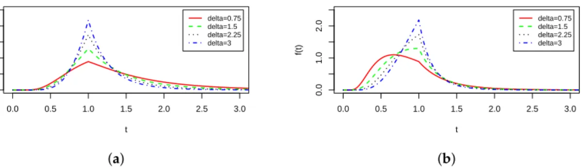
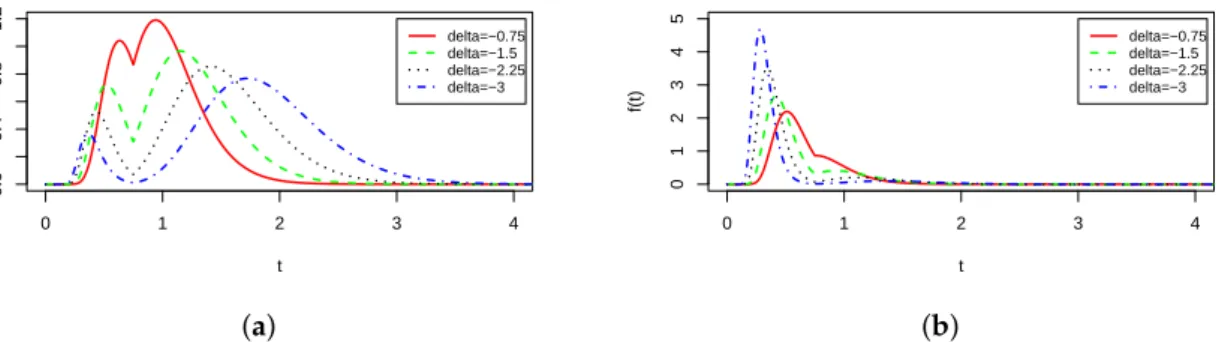
Figures1and2depict the behaviour of (8) for some values of parameters, illustrating that it can
be bimodal for some combinations of them.
2.1. Interpretation of Parameters.
In both figures the values of parametersαandβare fixed. We study the effects of
(i) λpositive versusλnegative.
(ii) Increasingδ>0 in Figure1. Decreasingδ<0 in Figure2.
Figure1suggests that, forαandβfixed, if a positive value ofδis considered then we have a
unimodal distribution and the peak of the distribution increases whenδincreases:δ=0.75 (red solid
line),δ=1.5 (green dashed line), . . . ,δ=3 (blue dashed dotted line). This happens for positive and
negative values ofλ.
On the other hand, in Figure2, we have different situations. This plot suggests that, forαandβ
fixed, if a negative value ofδis considered then a bimodal distribution can be obtained. For positive
λ, ifδdecreases:δ= −0.75 (red solid line),δ=−1.5 (green dashed line), . . . ,δ=−3 (blue dashed
dotted line), then the peaks decrease and bimodality becomes more accentuated. For negativeλ, ifδ
decreases, then main peak increases and bimodality becomes less accentuated.
Also, note in Figures1and2, that in the FBS model the pdf for negativeλis no longer the specular
image of plot for positiveλ.
0.0 0.5 1.0 1.5 2.0 2.5 3.0 0.0 1.0 2.0 FBS pdf's: lambda=1 t f(t) delta=0.75 delta=1.5 delta=2.25 delta=3 (a) 0.0 0.5 1.0 1.5 2.0 2.5 3.0 0.0 1.0 2.0 FBS pdf's: lambda=−1 t f(t) delta=0.75 delta=1.5 delta=2.25 delta=3 (b)
Figure 1.FBS distributions forα=0.75, β=1 (both fixed). In (a)λ=1 versus (b)λ=−1. Increasing
values ofδ>0:δ=0.75 (red solid line), 1.5 (green dashed line), 2.25 (black dotted line) and 3.0 (blue
0 1 2 3 4 0.0 0.4 0.8 1.2 FBS pdf's: lambda=0.5 t f(t) delta=−0.75 delta=−1.5 delta=−2.25 delta=−3 (a) 0 1 2 3 4 0 1 2 3 4 5 FBS pdf's: lambda=−0.5 t f(t) delta=−0.75 delta=−1.5 delta=−2.25 delta=−3 (b)
Figure 2.Flexible Birnbaum–Saunders (FBS) distributions forα=0.30, β=0.75 (both fixed). In (a) λ=0.5 versus (b)λ=−0.5. Decreasing values ofδ<0:δ=−0.75 (red solid line),−1.5 (green dashed
line),−2.25 (black dotted line) and−3.0 (blue dashed and dotted line).
2.2. Properties
Next, important properties of the FBS model are presented. First an explicit expression for the cdf is given in terms of the cdf of a bivariante normal distribution.
Proposition 1. Let T∼FBS(α,β,δ,λ). Then the cdf of T is
FT(t) = cδΦBNλ λδ √ 1+λ2,at−δ , if 0<t<β cδhΦBNλ λδ √ 1+λ2,−δ +ΦBN λ −√λδ 1+λ2,at+δ −ΦBNλ −√λδ 1+λ2,δ i , if t≥β, (9)
where ΦBNλ(x,y) is the cdf of a bivariate normal distribution, with mean vector µ
0 = (0, 0) and covariance matrix Ωλ= 1 ρλ ρλ 1 ! where ρλ=−√λ 1+λ2 . (10)
Proof. It can be seen in AppendixA.
Next some particular cases of interest forλandδparameters are discussed. Results about the
shape offT(·)are included.
2.2.1. Effect ofλ.
Corollary 1. Let T∼FBS(α,β,δ,λ). Ifλ=0then the cdf of T is
FT(t) = ( c δ 2Φ(at−δ), if 0<t<β cδ 2 {Φ(at+δ) +1−2Φ(δ)}, if t≥β. (11)
Proof. Ifλ=0 thenρλ, defined in (10), is equal to zero, and since in the bivariate normal distribution
uncorrelation implies independence, we have that
ΦBNλ=0(x,y) =Φ(x)Φ(y), ∀(x,y).
Taking into account thatΦ(0) =1/2 andΦ(−δ) =1−Φ(δ), we have that (9) reduces to (11).
Result in Corollary1corresponds to the model studied in [22].
2.2.2. Effect ofδ.
Corollary2is a particular case of models studied in [15]. 2.2.3. Shape of fT(·).
Proposition 2. Let T∼FBS(α,β,δ,λ).Then the pdf given in (8) is nondifferentiable at t=β.
Proof. It follows from (8), by noting that ift=βthenat=0 and the absolute value function is not
differentiable at zero.
Proposition 3. Let T∼FBS(α,β,δ,λ).The pdf given in (8) can be bimodal. The modes are the solution of the following non-linear equations.
1. 0<t1∗<βsolution of at1 =δ + λ φ(λat1) Φ(λat1) + a 00 t1 n a0t1o2 . (12) 2. t∗2>βsolution of at2 =−δ + λ φ(λat2) Φ(λat2) + a 00 t2 n a0t 2 o2 , (13)
With atgiven in (6), a0tand a00t the first and second derivatives of atwith respect to t, respectively.
Proof. It is given in AppendixA.
Comments on the use of (12) and (13) are included in AppendixA, RemarkA1.
Remark 1. Equations obtained in (12) and (13) are similar to those we have in the skew normal and BS model. 1. Let Z ∼ SN(λ), λ ∈ R. Then Z is unimodal and the mode, z∗, is given by the solution of the
non-linear equation
z=λφ(λz) Φ(λz) .
2. Let T ∼ BS(α,β),α,β > 0. Then T is unimodal and the mode, t∗, is given by the solution of the non-linear equation
−ata0t
2
+a00t =0.
Next it is shown that the p-th quantile ofT can be given in terms of the pthquantile of the
FSN(δ,λ). Also it is proved that the FBS model is closed under change of scale and reciprocity.
Theorem 1. Let T∼FBS(α,β,δ,λ), withα, β∈R+andδ, λ∈R. Then
(i) Let tpbe the pth quantile of T ,0< p<1.
tp=β α 2zp+ r α 2zp 2 +1 !2 (14)
where zpdenotes the pth quantile of Z∼FSN(δ,λ). (ii) kT ∼FBS(α,kβ,δ,λ)for k>0.
(iii) T−1∼FBS(α,β−1,δ,−λ). Proof. It can be seen in AppendixA.
2.2.4. Lifetime Analysis
The BS model is commonly used to explain survival and material resistance data. The survival and risk (or hazard) functions are important indicators in such fields. For the FBS model these functions are given next.
Proposition 4. Let T∼FBS(α,β,δ,λ)withα, β∈R+andδ, λ∈R. Then
(i) The survival function is S(t) =P[T>t] =1−FT(t)with FT(·)given in (9).
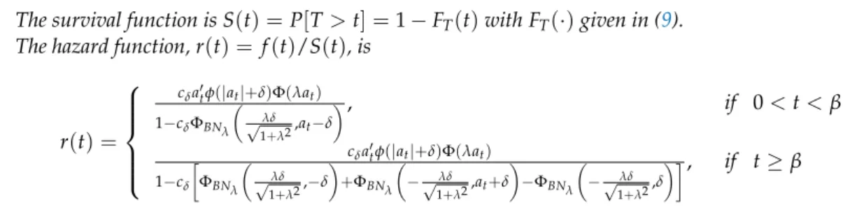
(ii) The hazard function, r(t) = f(t)/S(t), is
r(t) = cδa0tφ(|at|+δ)Φ(λat) 1−cδΦBNλ λδ √ 1+λ2 ,at−δ , if 0<t<β cδa0tφ(|at|+δ)Φ(λat) 1−cδ ΦBNλ λδ √ 1+λ2 ,−δ +ΦBNλ −√λδ 1+λ2 ,at+δ −ΦBNλ −√λδ 1+λ2 ,δ , if t≥β
withΦBNλ(·)the cdf of the bivariate normal given in Proposition1.
In Figure3, the hazard function for those pdf’s considered in Figures1and2are plotted. These
graphs show that, for the FBS distribution, the hazard function admits a variety of shapes, which is interesting from an applied point of view.
0.5 1.0 1.5 2.0 2.5 3.0 1 2 3
Figure 1
(
a
)
0.5 1.0 1.5 2.0 2.5 3.0 1 2 3 4 5Figure 1
(
b
)
0.5 1.0 1.5 2.0 2.5 3.0 1 2 3 4 5 6Figure 2
(
a
)
0.5 1.0 1.5 2.0 2.5 3.0 2 4 6 8Figure 2
(
b
)
Figure 3.Hazard function of the FBS distribution for plots corresponding to Figure 1 (a), (b):α=0.75, β=1 (both fixed),δ=0.75 (red solid line), 1.5 (green dashed line), 2.25 (black dotted line) and 3.0
(blue dashed dotted line), in (a)λ=1 versus (b)λ=−1. For plots corresponding to Figure 2 (a), (b): α=0.30,β=0.75 (both fixed),δ=−0.75 (red solid line), –1.5 (green dashed line), –2.25 (black dotted
line) and –3.0 (blue dashed dotted line), in (a)λ=0.5 versus (b)λ=−0.5.
Remark 2. More complicated hazard functions than the traditional ones are obtained when we are dealing with models with complex structure, as it happens with the FBS. For instance, in Figure3, we have two situations: 1. r(t)corresponding to Figure1a,b. These are, first, quickly increasing, later decreasing more slowly or even
in a flat way. It can be applied in practical situations in which the risk of failure increases quickly until certain point in which its behaviour becomes flatter. As [23] points out, the flat area is very interesting in survival analysis and reliability contexts.
2. r(t)corresponding to Figure2a,b are increasing-decreasing-increasing. This kind of hazard functions has been recently introduced and discussed in literature, due to its interest in reliability of systems, see for instance [23] or [24] (and references therein). In plot for Figure2b, r(t)is (quickly) increasing—or (quickly) decreasing. On the other hand, for Figure2a the initial effect increasing—decreasing is less accentuated. 3. Moments and Maximum Likelihood Estimation
Moments of the FBS model can be obtained from the moments of the flexible skew-normal model
given in [2]. The following results present important properties relating those distributions, and the
expressions for the first moment and variance in the FBS model.
Theorem 2. Let T∼FBS(α,β,δ,λ)and Z∼FSN(δ,λ).ThenE(Tr), r=0, 1, . . ., always exists. Moreover
E(Tr) = β r 4r 2r
∑
k=0 2r k E " (αZ)k α2Z2+4 2r−k2 # , r=0, 1, . . . . (15)Proof. From (7), we can write
T= β 4 αZ+ α2Z2+4 1/22 . Taking expectation of the rth-power of T
E(Tr) = β r 4rE " αZ+ α2Z2+4 1/22r # . (16)
From (16), note that forr=0, 1, . . .,E(Tr)exists if and only ifE(Z2r)exists. On the other hand, it
can be seen in [2] thatE(Z2r)always exists, and thereforeE(Tr)too.
Finally note that (15) is the result of applying the binomial formula to (16).
Next, explicit expressions for the expected value and variance ofT ∼FBS(α,β,δ,λ)are given.
In these expressions,κj=ESFN
Zj 2 √ α2Z2+4 withZ∼FSN(δ,λ).
Theorem 3. Let T∼FBS(α,β,δ,λ). Then
E(T) =β 1+ακ1+ α2 2 cδ n (1+δ2)(1−Φ(δ))−δφ(δ) o , (17) E(T2) =β2 7α4cδ 16 (3+6δ2+δ4)(1−Φ(δ))−δ(5+δ2)φ(δ) +α3κ3+2ακ1+1 +2α2β2cδ (1+δ2)(1−Φ(δ))−δφ(δ) and Var(T) =β2 7 α4cδ 16 (3+6δ2+δ4)(1−Φ(δ))−δ(5+δ2)φ(δ) +α3κ3−α2κ1+1 −α 2β2c δ 4 (1+δ2)(1−Φ(δ))−δφ(δ) α2cδ (1+δ2)(1−Φ(δ))−δφ(δ) +4(1−ακ1) whereκj=EFSN Zj 2 √ α2Z2+4 and Z∼FSN(δ,λ).
Proof. These results follows from Theorem2and the expressions ofκj, which have been computed by
using the results for moments ofZ∼FSN(δ,λ)obtained in [2].
As illustration, note that for the caser=1, (15) reduces to
E(T) = β 4 h E(α2Z2+4) +2E (αZ) p α2Z2+4) +E(α2Z2) i = β 1+ακ1+ α2 2 E(Z 2) ,
it can be seen in [2] thatE(Z2) =cδ(1+δ2) (1−Φ(δ))−δφ(δ)), and so (17) is obtained.
3.1. Maximum Likelihood Estimators
Parameter estimation in the BS model has been the topic of interest in many papers. Among
others, we mentioned [25–27]. To estimate the parameters in the usual BS model, the modified moment
method (MME) and maximum likelihood (MLE) are commonly used. To start the maximum likelihood approach moment estimators are used which are given by
ˆ βM= √ sr, αˆM= s 2 rs r−1 . where s = 1n∑ni=1ti and r = 1 n∑ni=1t1i −1
are the sample (arithmetic) and harmonic mean, respectively. Relevant aspects of this distribution such as its robustness with respect to parameter
estimation andO(n−1)bias corrections for MLEs, can be seen in [25–27].
In the following, we discuss MLE estimation for the FBS model in depth. Thus, given
n observations independent and identically distributed, T1,T2, ...,Tn, with Ti ∼ FBS(α,β,δ,λ),
the log-likelihood function for the parameter vectorθ= (α,β,δ,λ)0is given by
`(θ) =−n log(α) +1 2log(β) +log(1−Φ(δ)) −3 2 n
∑
i=1 log(ti) + n∑
i=1 log(ti+β) −1 2 n∑
i=1 (a2ti+2δ|ati|+δ 2) +∑
n i=1 log(Φ(λati)). (18)To maximizel(θ)inθ, consider the first derivatives ofl(θ)with respect toα,β,δandλ, denoted
as ˙lα, ˙lβ, ˙lδand ˙lλ, respectively. From ˙lα =0, ˙lβ =0, ˙lδ =0 and ˙lλ =0, the likelihood equations are
given by −n+ n
∑
i=1 a2ti−δ n∑
i=1 |ati| −λ n∑
i=1 ati φ(λati) Φ(λati) = 0 (19) − n 2β+ n∑
i=1 1 ti+β + 1 2αβ3/2 n∑
i=1 sgn(ati) (|ati|+δ)−λ φ(λati) Φ(λati) ti+β √ ti = 0 (20) δ− φ(δ) 1−Φ(δ) = − 1 n n∑
i=1 |ati| (21) n∑
i=1 ati φ(λati) Φ(λati) = 0 (22)in whichsgn(·)denotes thesignfunction.
The solution to the previous system of equations must be obtained by iterative methods such as the Newton-Raphson or quasi-Newton procedures, which can be implemented using the statistical software R, [28].
As initial estimates ofαandβcan be proposed the estimates of these parameters obtained in the
basic BS model, denoted asbα0andβb0. These estimates can be plugged into (21) and (22) to obtain
preliminar estimates ofδandλ,bδ0andbλ0, and so, start the recursion.
3.2. Expected and Observed Information Matrices
Recall that, the Fisher information matrix is given by
I(θ) = ji,ji,j=α,β,δ,λ,
which entries are equal to minus the second partial derivatives of the log-likelihood function given
in (18) with respect to the parameters in the model. They are denoted asjαα =− ∂
2 ∂α2l(θ), and so on. So we have jαα =− n α2+ 1 α2 n
∑
i=1 3a2ti +2δ|ati| + λ α2 n∑
i=1 atiwi(2+λatiBi), jβα =− 1 α3β2 n∑
i=1 β2−t2i ti ! + 1 2α2β3/2 n∑
i=1 (δsgn(ati) +λwi(−1+λatiBi)) ti+β √ ti , jββ=− n 2β2+ n∑
i=1 1 ti+β+ 1 α2β3 n∑
i=1 ti+ 1 4αβ5/2 n∑
i=1 (δsgn(ati)−λwi) 3ti+β √ ti + λ 2 4α2β3/2 n∑
i=1 wiBi ti+β √ ti 2 , jδα=− 1 α n∑
i=1 |ati|, jδβ=− 1 2α2β3/2 n∑
i=1 sgn(ati) ti+β √ ti , jλα= 1 α n∑
i=1 atiwi(1−λatiBi), jλβ= 1 2αβ3/2 n∑
i=1 wi(1+λatiBi) ti+β √ ti , jδδ=n(wδ(δ−wδ) +1), jδα=jδβ=jλδ =0, jλλ= n∑
i=1 a2tiwiBi wherew= φ(λat) Φ(λat), wδ =φ(δ)/(1−Φ(δ)) and B=λat+w.The Fisher (expected) information matrix would be obtained by computing the expected values of
the above second derivatives. Taking in this matrixδ=λ=0, that is,T∼BS(α,β), and, using results
in [21], we have I(θ) = 2 α2 0 − 1 α q 2 π 0 0 α−2β−2 1+αq√(α) 2π 0 √1 2π 1 αβ3/2A1(t) −α1qπ2 0 1−π2 0 0 √1 2π 1 αβ3/2A1(t) 0 2 π , where A1(t) = E t i+β √ ti , q(α) = α q 2 π − πexp(2 α2)
2 er f c(2α), with er f c(·) the error function, i.e.,
er f c(x) = √2
π
R∞
x exp(−t2)dt, see [29].
Hence, for large samples, the MLE,bθ, ofθis asymptotically normal, that is, √
nbθ−θ
L
−→N4(0, I(θ)−1),
resulting that the asymptotic variance of the MLE, ˆθ, is the inverse of Fisher information matrixI(θ).
Since the parameters are unknown, usually the observed information matrix is considered where the unknown parameters are estimated by ML.
Asymptotic confidence intervals for the parameters in the FBS model can be obtained from these results.
4. Numerical Illustrations
The numerical illustrations introduced next are aimed to show that the FBS model can be an alternative to modelling unimodal or bimodal data from different areas. First illustration is related to nickel content in soil samples analyzed at the Mining Department (Departamento de Minas) of Universidad de Atacama, Chile. We start by showing that both, BS and skew-BS (SBS) models are not able to capture bimodality present in this data set. Thus, the FBS model turned out to be a good option, to fit the data even better than a mixture of two normal distributions, which is another competing alternative to fit bimodal data. Second illustration is related to air pollution in New York city in USA,
which was previously analyzed in [16,30]. In this case, it is shown that FBS model again provides
a better fit than BS and SBS. As competing model the extended Birnbaum-Saunders (EBS) is also
considered. Recall that theEBS(α,β,σ,ν,λ)is a five-parameter model proposed in [16] where the
parameterσaffects the kurtosis;νandλaffect the skewness; andαandβthe shape and scale as in the
usual BS model. We highlight that, for this dataset, theFBS(α,β,δ,λ)model provides a better fit than
that given by theEBS(α,β,σ,ν,λ)in [16] with the merit of using less parameters.
4.1. Nickel Concentration
For illustrative purposes, we apply the FBS model to a data set related to nickel content in soil samples. This data set encompasses 85 observations of the variable concentration of nickel with sample mean = 21.588, sample standard deviation = 16.573, sample asymmetry = 2.392 and sample kurtosis = 8.325, much higher than expected with the ordinary BS distribution.
4.1.1. FBS versus the BS and SBS distributions
To fit the nickel concentration variable, we use the BS, skew BS (SBS) and FBS models. Using
function optim from the R-package, [28], the following point estimates (and their standard errors) are
obtained for each of the three models under consideration
BS model: ˆα=0.789(0.060) and ˆβ=16.382(1.296).
SBS model: ˆα=1.073(0.201), ˆβ=8.841(1.998)and ˆλ=1.252(0.590).
FBS model: ˆα=0.870(0.104), ˆβ=5.072(0.763), ˆδ=−1.520(0.282)and ˆλ=1.405(0.341).
The bimodal hypothesis can be formally tested as follows
H0:δ=0 versus H1:δ6=0,
which is equivalent to compare models SBS versus FBS. Given the nonsigularity of the Fisher information matrix, and since these models are nested, we can consider the likelihood ratio statistics, namely
Λ1=LSBS(bα,βb,bλ)/LFBS(bα,βb,δb,bλ).
It is obtained−2 log(Λ1) = 5.618, which is greater than the 5% chi-square critical value with
one degree of freedom (df), which is equal to 3.84. Therefore, the null hypothesis of no-bimodality is rejected at the 5% critical level, leading to the conclusion that FBS model fits better than the unimodal SBS model to the nickel concentration data.
To compare the FBS model with the BS model, consider to test the null hypothesis of a BS distribution versus a FBS distribution, that is
H0: (δ,λ) = (0, 0) vs H1: (δ,λ)6= (0, 0)
using the likelihood ratio statistics based on the ratio Λ2 = LBS(bα,βb)/LFBS(bα,βb,δb,bλ). After
substituting the estimated values, we obtain −2 log(Λ2) = 7.628, which is greater than the 5%
chi-square critical value with 2 df, which is 5.99. Therefore the FBS is preferred to BS model for this data set.
4.1.2. FBS versus a Mixture of Normal Distributions
Another model widely applied in such situations of bimodality is the mixture of two normal distributions. The normal mixture model is given by:
f(x;µ1,σ1,µ2,σ2,p) =p f1(x,µ1,σ1) + (1−p)f2(x;µ2,σ2) (23)
where fjis a normal distribution with parameters(µj,σj),j=1, 2 and 0< p<1. (23) is denoted by
MN(µ1,σ1,µ2,σ2,p).
To compare FBS model with the MN model, we propose the Akaike information criterion (AIC),
see [31], namelyAIC=−2ˆ`(·) +2k, the modified AIC criterion (CAIC), typically called the consistent
AIC, namelyCAIC = −2ˆ`(·) + (1+log(n))kand the Bayesian Information Criterion, BIC,BIC =
−2ˆ`(·) +log(n)k, wherekis the number of parameters and ˆ`(·)is the log-likelihood function evaluated
at the MLEs of parameters. The best model is the one with the smallest AIC or CAIC or BIC.
Now we compare the FBS with MN(µ1,σ1,µ2,σ2,p). The estimated mixture model is
MN(15.348, 6.622, 40.908, 21.960, 0.755)
withAIC=674.849, CAIC=692.061 andBIC=687.062. On the other hand, for the FBS model, we
haveAIC=671.859, CAIC=685.628 andBIC=681.630. According to these criteria, the FBS model
provides a better fit to the data of nickel concentration. 4.1.3. FBS versus a Mixture of Log-Normal Distributions
Following reviewer’s recommendations, a mixture of two log-normal distributions is also
considered. The log-normal mixture model will be given by (23) with fj the pdf of a log-normal
distribution with parameters(µj,σj),j=1, 2 and 0< p<1, and it is denoted by MLN(µ1,σ1,µ2,σ2,p).
The estimated mixture model is
MLN(2.829, 0.177, 2.8275, 0.877, 0.327)
with AIC = 663.571, CAIC = 680.784 and BIC = 675.784. All of them are less than those
corresponding to FBS. So, according to these criteria, the mixture ot two log-normal distributions provides a better fit to this dataset than the FBS model.
This discussion illustrates that, quite often, the final selection of a model is a matter of choice. FBS model can be considered as appropriate if we want to use a more parsimonious model, and this is better than other BS models and a mixture of two normal distributions. On the other hand, based on AIC, CAIC and BIC, the mixture of two log-normal would be preferred but this model has more parameters than the FBS distribution and may present problems of identifiability. Anyway, the final choice must be properly justified.
Figure4 depicts maximized likelihoods and empirical cdf for variable nickel concentration
t density 0 20 40 60 80 100 0.00 0.01 0.02 0.03 0.04 0.05 (a) 0 20 40 60 80 100 120 0.0 0.2 0.4 0.6 0.8 1.0 t Cum ulativ e distr ib ution (b)
Figure 4.(a) Plots for FBS, (solid line), MLN (dashed line), BS (dotted line) and SBS (dotted and dashed line) models . (b) Empirical cdf with estimated FBS cdf (dashed line) and estimated BS cdf (dotted line).
Remark 3. Going through the origin of this data set, the bimodal behavior of the nickel concentration statistical model seems to be due to the fact that the samples were taken according to different lithologies. Lithology classifies according to the physical and chemical elements in rock formation. Mining operations found different lithologies in these samples, as it is depicted in Figure4.
4.2. Air Pollution
The concentration of average air pollutants has been used in epidemiological surveillance as an indicator of the level of atmospheric contamination. Among its associated adverse effects in humans, diseases such as bronchitis are found. The distribution of this concentration has a bias to the right, and is always positive. It is typically assumed that the data on air pollutant concentrations are uncorrelated
and independent and thus they do not require the diurnal or cyclic trend analysis, see [32]. The data
set studied in this section corresponds to daily measures of ozone levels (inppb=ppm×1000) in the
city of New York, USA, from May to September, 1973, collected by the New York State Conservation Department. The sample mean, standard deviation, asymmetry and kurtosis coefficients are given, respectively, by 42.129, 32.987, 1.209 and 1.112.
4.2.1. FBS versus the BS and SBS Distributions
Maximum likelihood estimators, their estimated standard errors (in parenthesis), for the BS, SBS and FBS models, were computed, the results are:
BS model: ˆα=0.982(0.064) and ˆβ=28.031(2.265).
SBS model: ˆα=1.270(0.235), ˆβ=14.831(4.019)and ˆλ=1.066(0.533).
FBS: ˆα=5.160(0.481), ˆβ=78.000(0.008), ˆδ=3.991(0.050)and ˆλ=−9.135(2.417).
For this data set, the log-likelihood ratio statistics to test BS vs FBS and SBS vs FBS are given by
−2 log(Λ1) =12.812 and −2 log(Λ2) =5.828,
which are greater than the corresponding 5% critical values from the chisquare distribution, which are 5.99 (with 2 df) and 3.84 (with one df), respectively. So, we can conclude that the unimodal FBS model provides a better fit to this dataset than BS and FBS models.
4.2.2. FBS versus the Extended BS (EBS) Model
Fitting the five-parameter EBS model, EBS(α,β,σ,ν,λ), proposed in [16] as the best for this
dataset, and whose point estimates for the parameters and summaries for comparison are equal to
EBS(0.780, 0.596, 3.618,−3.539,−0.096),
CAIC = 1111.154 andBIC = 1106.154. On the other hand, for the FBS model, it was obtained
CAIC = 1108.396 andBIC = 1104.396. Then, according to the CAIC and BIC criteria, FBS model
presents the best fit to this data set dealing with the daily ozone level concentration in the atmosphere.
Figure5depicts the histograms and the fitted density curves for the data set studied and empirical
cdf for variable daily ozone level concentration in the atmosphere, while the dashed line corresponds to the cfd for FBS model.
t density 0 50 100 150 0.000 0.005 0.010 0.015 0.020 0.025 (a) 0 50 100 150 0.0 0.2 0.4 0.6 0.8 1.0 t Cum ulativ e distr ib ution (b)
Figure 5.(a) Plots for FBS, (solid line), BS (dotted line), SBS (dashed line) and EBS (dotted and dashed line) models. (b) Empirical cdf with estimated FBS cdf (dashed line).
5. Conclusions
We have introduced a new family of distributions able to model skewness, unimodality and bimodality in the BS distribution. We have discussed several of its properties. Explicit expressions for the cdf are given in terms of the cdf of a bivariate normal variable. Non-linear equations to obtain the modes of this distribution are provided. The estimation of parameters is carried out via maximum likelihood. We highlight that the ML equations must be solved by using iterative methods. The information matrix is non-singular and therefore likelihood ratio tests to compare this model with other nested models can be implemented. The interest and flexibility of our proposal is supported with two illustrations to real data in which we show that:
(i) the FBS model provides consistently better fits than the BS and SBS models (they can be considered relevant precedents of our proposal)
(ii) the FBS distribution can improve the fit provided by other competing models designed to deal with bimodality (such as a mixture of normal distributions). It can also perform better for unimodal situations in which a generalized BS model with skewness parameters must be applied,
such as the EBS model proposed in [16]. We highlight that in both situations FBS provides a
better fit with a more parsimonious model (less number of parameters), and the problem of identifiability of mixtures can be circumvented.
Therefore the outcome of these practical demonstrations show that the new family is very flexible and widely applicable.
Author Contributions:All the authors contributed significantly to the present paper.
Funding: The research of G. Martínez-Flórez was supported by Grant Proyecto Universidad de Córdoba: Distribuciones de probabilidad asimétrica bimodal con soporte positivo (Colombia). The research of I. Barranco-Chamorro was supported by Grant CTM2015-68276-R (Spain). H.W. Gómez was supported by Grant SEMILLERO UA-2019 (Chile).
Acknowledgments:The authors would like to thank the editor and the anonymous referees for their comments and suggestions, which significantly improved our manuscript.
Conflicts of Interest:The authors declare no conflict of interest.
Appendix A
Proof of Proposition1(cdf in the FBS model). From Equation (7),T is a monotonically increasing
function ofZ∼FSN(δ,λ). Therefore the cdf ofTis given by
FT(t) =FZ(at) (A1)
whereFZ(·)denotes the cdf ofZandatwas given in (6).
(i) First, we obtain the cdf ofZ∼FSN(δ,λ)
It can be seen in Gómez et al. [2], Proposition 4, that the pdf ofZ∼FSN(δ,λ)is
fZ(z) =
(
cδφ(z−δ)Φ(λz), ifz<0 cδφ(z+δ)Φ(λz), ifz≥0.
Let us consider the case forz<0
FZ(z) = Z z
−∞fZ(t)dt =
Z z
−∞cδφ(t−δ)Φ(λt)dt
By making the change of variablev=t−δ, and later, taking into account thatΦ(·)is the cdf of a
N(0, 1)distribution, we have that
FZ(z) =cδ Z z−δ −∞ φ(v)Φ(λ(v+δ))dv=cδ Z z−δ −∞ Z λ(v+δ) −∞ φ(v)φ(s)dsdv (A2)
The integrand in (A2) is the joint pdf of two independentN(0, 1)rv’s,(S,V), i.e.,
S V ! ∼N2 0 0 ! , 1 0 0 1 !!
Note that (A2) can be rewritten as
FZ(z) =cδ Pr[S−λV≤λδ, V≤z−δ] =cδ Pr S−λV √ 1+λ2 ≤ √ λδ 1+λ2 , V≤z−δ =cδΦBNλ λδ √ 1+λ2 ,z−δ (A3)
whereΦBNλ(x,y)denotes the cdf of a bivariate normal distribution, with mean vectorµ
0 = (0, 0)and
covariance matrixΩλgiven in (10).
Forz>0, we have that
FZ(z) = Z 0 −∞ fZ(t)dt + Z z 0 fZ(t)dt =FZ(0) +cδ Z z 0 φ (t+δ)Φ(λt)dt. (A4)
From (A3), it follows that FZ(0) = lim z→0−FZ(z) = cδΦBNλ λδ √ 1+λ2 , −δ (A5)
On the other hand, proceeding similarly to the previous case (change of variablev=t+δ), it can
be proved that Z z 0 φ (t+δ)Φ(λt)dt=Pr S− λV √ 1+λ2 ≤ −√ λδ 1+λ2 , δ<V≤z+δ =ΦBNλ −√ λδ 1+λ2 ,z+δ −ΦBNλ −√ λδ 1+λ2 ,δ (A6)
Therefore, from (A3)–(A6), we have just proved that the cdf ofZis
FZ(z) = cδΦBNλ λδ √ 1+λ2,z−δ , ifz<0 cδ h ΦBNλ λδ √ 1+λ2,−δ +ΦBN λ −√λδ 1+λ2, z+δ −ΦBNλ −√λδ 1+λ2, δ i , ifz≥0 (A7)
(ii) Finally, the expression for the cdf of T ∼ FBS(α,β,δ,λ) given in (9) follows from (A1)
and (A7).
Proof of Proposition3(Modes in the FBS model). Recall that, from (A1), the pdf ofTis given by
fT(t) = fZ(at)a0t=cδa
0
tφ(|at|+δ)Φ(λat)
where fZ(·)denotes the pdf ofZ∼FSN(δ,λ),atwas given in (6) and
a0t=
∂ ∂tat=
t−3/2β−1/2
2α (t+β). (A8)
Forat<0, or equivalently 0<t<β, consider the first derivative with respect totof fT(·)and
equating to zero, we have
fT0(t) =cδ
∂ ∂t
a0tφ(−at+δ)Φ(λat) =0 (A9)
By using thatφ0(z) =−zφ(z), it can be proved that (A9) is equivalent to
a0t 2 [(δ−at)Φ(λat) +λφ(λat)] +a 00 tΦ(λat) =0 (A10)
Sincea0t>0,∀t>0 (β>0), we have that (A10) is equivalent to (12).
Similarly, forat>0, i.e.,t>β, from fT0(t) =cδ∂t∂ {a0tφ(at+δ)Φ(λat)}=0 , (13) is obtained.
Remark A1(Comments to Proposition3). In order to illustrate the use of Equations (12) and (13) next cases are considered.
1. Consider the pdf given in Figure1a, caseα=0.75,β=1,λ=1,δ=0.75. In this setting there do not exist t∗1∈(0,β)and t∗2>βsatisfying (12) and (13), respectively. It can be checked than the distribution is unimodal and the mode is atβ.
2. Figure1b, caseα=0.75,β=1,λ=−1,δ=0.75. There exists t∗1 ∈(0,β)satisfying (12) and there does not exists t∗2>βsatisfying (13). Then the distribution is unimodal and the mode is at t∗1.
3. Figure2a,b, in all cases under consideration, there exist t∗1∈(0,β)and t∗2>βsatisfying (12) and (13). Then the distribution is bimodal and the modes are t∗1and t∗2.
Proof of Theorem1(pthquantile, change of scale and reciprocity). (i) (14) follows from the fact
that (7) is one-to-one function preserving the order fromRtoR+.
(ii) Note that the pdf ofTcan be rewritten as
fT(t) =cδa
0
t(α,β)φ(|at(α,β)|+δ)Φ(λat(α,β)) (A11)
withcδ = (1−Φ(δ))−1,at=at(α,β)given in (6) and
a0t=a0t(α,β) =
∂
∂tat(α,β) =
t−3/2β−1/2
2α (t+β). (A12)
LetY = kT withk > 0. By applying the Jacobian technique fY(y) = |J|fT(yk;α,β,δ,λ)with
|J|= 1k. From (6),ay/k(α,β) =ay(α,kβ), and from (A12)
|J|a0y/k(α,β) = y −3/2(kβ)−1/2 2α (y+kβ) =a 0 y(α,kβ). Therefore fY(y) =cδa 0 y(α,kβ)φ(|ay(α,kβ)|+δ)Φ(λay(α,kβ)), i.e.,Y∼FBS(α,kβ,δ,λ).
(iii) Let beY=T−1. In this case|J|=Y−2,a
y−1(α,β) =−ay(α,β−1), and|J|a0y−1(α,β) =a0y(α,β−1). Therefore fY(y) =|J|fT(y−1;α,β,δ,λ) =cδay0(α,β−1)φ |ay(α,β−1)|+δ Φ−λay(α,β−1) , i.e.,Y=T−1∼FBS(α,β−1,δ,−λ). References
1. Birnbaum, Z.W. Effect of linear truncation on a multinormal population.Ann. Math. Statist.1950,21, 272–279. [CrossRef]
2. Gómez, H.W.; Elal-Olivero, D.; Salinas, H.S.; Bolfarine, H. Bimodal Extension Based on the Skew-normal Distribution with Application to Pollen Data.Environmetrics2009,22, 50–62. [CrossRef]
3. Lehmann, E.L. The power of rank tests.Ann. Mathematical Stat.1953,24, 23–43. [CrossRef]
4. Roberts, C. A Correlation Model Useful in the Study of Twins. J. Am. Stat. Assoc. 1966,61, 1184–1190. [CrossRef]
5. O’Hagan, A.; Leonard, T. Bayes estimation subject to uncertainty about parameter constraints.Biometrika 1976,63, 201–203. [CrossRef]
6. Azzalini, A. A class of distributions which includes the normal ones.Scand. J. Stat.1985,12, 171–178. 7. Arnold, B.C.; Gómez, H.W.; Salinas, H.S. On multiple contraint skewed models’.Statistics 2009,43, 279–293.
[CrossRef]
8. Bolfarine, H.; Martínez–Flórez, G.; Salinas, H.S. Bimodal symmetric-asymmetric families.Commun. Stat. Theory Methods2018,47(2), 259–276. [CrossRef]
9. Durrans, S.R. Distributions of fractional order statistics in hydrology.Water Resour. Res.1992,28, 1649–1655. [CrossRef]
10. Pewsey, A.; Gómez, H.W.; Bolfarine, H. Likelihood-based inference for power distributions. Test2012, 21, 775–789. [CrossRef]
11. Chan, J.; Choy, S.; Makov, U.; Landsman, Z. Modelling insurance losses using contaminated generalised beta type-II distribution.ASTIN Bull.2018,48, 871–904.
12. Birnbaum, Z.W.; Saunders, S.C. Estimation for a family of life distributions with applications to fatigue. J. Appl. Probab.1969,6, 328–347. [CrossRef]
13. Birnbaum, Z.W.; Saunders, S.C. A New Family of Life Distributions. J. Appl. Probab. 1969,6, 319–327. [CrossRef]
14. Díaz-García, J.A.; Leiva-Sánchez, V. A new family of life distributions based on the elliptically contoured distributions.J. Statist. Plann. Inference2005,128, 445–457. [CrossRef]
15. Vilca-Labra, F.; Leiva-Sanchez, V. A new fatigue life model based on the family of skew-elliptical distributions. Commun. Stat. Theory Methods2006,35, 229–244. [CrossRef]
16. Leiva, V.; Vilca-Labra, F.; Balakrishnan, N.; Sanhueza, A. A skewed sinh-normal distribution and its properties and application to air pollution.Commun. Stat. Theory Methods2010,39, 426–443. [CrossRef] 17. Castillo, N.O.; Gómez, H.W.; Bolfarine, H. Epsilon Birnbaum-Saunders distribution family: Properties and
inference.Stat. Pap.2011,52, 871–883. [CrossRef]
18. Gómez, H.W.; Olivares, J.; Bolfarine, H. An extension of the generalized Birnbaum- Saunders distribution. Stat. Probab. Lett.2009,79, 331–338. [CrossRef]
19. Reyes, J.; Barranco-Chamorro, I.; Gallardo, D.I.; Gómez, H.W. Generalized Modified Slash Birnbaum-Saunders Distribution.Symmetry2018,10, 724. [CrossRef]
20. Reyes, J.; Barranco-Chamorro, I.; Gómez, H.W. Generalized modified slash distribution with applications. Commun. Stat. Theory Methods2019, doi:10.1080/03610926.2019.1568484. [CrossRef]
21. Martínez-Flórez, G.; Bolfarine, H.; Gómez, H.W. An alpha-power extension for the Birnbaum-Saunders distribution.Statistics2014,48, 896–912. [CrossRef]
22. Olmos, N.M.; Martínez-Flórez, G.; Bolfarine, H. Bimodal Birnbaum-Saunders Distribution with Application to Corrosion Data.Commun. Stat. Theory Methods2017,46, 6240-6257. [CrossRef]
23. Shakhatreh, M.; Lemonte, A.; Moreno-Arenas, G. The log-normal modified Weibull distribution and its reliability implications.Reliab. Eng. Syst. Saf.2019,188, 6–22. [CrossRef]
24. Prataviera, F.; Ortega, E.M.M.; Cordeiro, G.M.; Pescim, R.R. A new generalized odd log-logistic flexible Weibull regression model with applications in repairable systems.Reliab. Eng. Syst. Saf.2018,176, 13–26. [CrossRef]
25. Ng, H.K.T.; Kundu, D.; Balakrishnan, N. Modified moment estimation for the two-parameter Birnbaum-Saunders distribution.Comput. Statist. Data Anal.2003,43, 283–298. [CrossRef]
26. Barros, M.; Paula, G.A.; Leiva, V. A new class of survival regression models with heavy-tailed errors: Robustness and diagnostics.Lifetime Data Anal.2008,14, 316–332. [CrossRef]
27. Lemonte, A.; Cribari-Neto, F.; Vasconcellos, K. Improved statistical inference for the two-parameter Birnbaum-saunders distribution.Comput. Stat. Data Anal.2007,51, 4656–4681. [CrossRef]
28. R Development Core Team.A Language and Environment for Statistical Computing; R Foundation for Statistical Computing: Vienna, Austria, 2017.
29. Gradshteyn, I.S.; Ryzhik, I.M.Table of Integrals, Series, and Products; Academic Press: New York, NY, USA, 2007. 30. Nadarajah, S. A truncated inverted beta distribution with application to air pollution data.Stoch. Environ.
Res. Risk Assess.2008,22, 285–289. [CrossRef]
31. Akaike, H. A new look at statistical model identification. IEEE Trans. Autom. Control1974,19, 716–723. [CrossRef]
32. Gokhale, S.; Khare, M. Statistical behavior of carbon monoxide from vehicular exhausts in urban environments.Environ. Model. Softw.2007,22, 526–535. [CrossRef]
c
2019 by the authors. Licensee MDPI, Basel, Switzerland. This article is an open access article distributed under the terms and conditions of the Creative Commons Attribution (CC BY) license (http://creativecommons.org/licenses/by/4.0/).