Data Assimilation and Inverse Problems

DRAFT

Andrew Stuart† and Armeen Taeb‡ *

† _{Department of Computational and Mathematical Sciences} ‡ _{Department of Electrical Engineering}

California Institute of Technology Pasadena, CA 91125

*

Email: [email protected], [email protected]

DRAFT

Introduction

Overview of the Notes

These notes are designed with the aim of providing a clear and concise introduction to the subjects of Inverse Problems and Data Assimilation, and their inter-relations, together with citations to some relevant literature in this area.

In its most basic form, inverse problem theory is the study of how to estimate model parameters from data. Often the data provides indirect information about these parameters, corrupted by noise. The theory of inverse problems, however, is much richer than just parameter estimation. For example, the underlying theory can be used to determine the effects of noisy data on the accuracy of the solution; it can be used to determine what kind of observations are needed to accurately determine a parameter; and it can be used to study the uncertainty in a parameter estimate and, relatedly, is useful, for example, in the design of strategies for control or optimization under uncertainty, and for risk analysis. The theory thus has applications in many fields of science and engineering.

To apply the ideas in these notes, the starting point is a mathematical model mapping the unknown parameters to the observations: termed the “forward” or “direct” problem, and often a subject of research in its own right. A good forward model will not only identify how the data is dependent on parameters, but also what sources of noise or model uncertainty are present in the postulated relationship between forward model and data. For example, if the desired forward problem cannot be solved analytically, then the forward model may be approximated by a simulation; in this case discretization may be considered as a source of error. Once a relationship between model parameters, sources of error, and data is clearly defined, the inverse problem of estimating parameters from data can be addressed. The theory of inverse problems can be separated into two cases: (1) the ideal case where data is not corrupted by noise and is derived from a known perfect model; and (2) the practical case where data is incomplete and imprecise. The first case is useful for classifying inverse problems and determining if a given set of observations can, in principle, provide exact solutions; this provides insight into conditions needed for existence, uniqueness, and stability of a solution. The second case is useful for the formulation of practical algorithms to learn about parameters, and uncertainties in their estimates, and will be the focus of these notes.

A model that has the properties: (a) a solution map exists, (b) is unique, and (c) its behavior changes continuously with input (stability) is termed “well-posed”. Conversely, a model lacking any of these properties is termed “ill-posed”. Ill-posedness is present is many inverse problems, and mitigating it is an extensive part of the subject. Out of the different approaches for formulating an inverse problem, the Bayesian framework naturally offers the ability to assess quality in parameter estimation, and also leads to a form of well-posedness at the level of probability distributions describing the solution.

DRAFT

The goal of the Bayesian framework is to find a probability measure that assigns a probability to each possible solution for a parameter𝑢, given the data 𝑦. Bayes formula states that

P(𝑢|𝑦) = 1

P(𝑦)P(𝑦|𝑢)P(𝑢).

It enables calculation of the posterior probability on𝑢|𝑦, P(𝑢|𝑦), in terms of the product of the data likelihoodP(𝑦|𝑢) and the prior information on the parameter encoded inP(𝑢). The likelihood describes the probability of the observed data𝑦, if the input parameter were set to be𝑢; it is determined by the forward model, and the structure of the noise. The normalization parameterP(𝑦) ensures that P(𝑢|𝑦) is a probability measure. There are five primary benefits to this framework: (a) it provides a clear theoretical setting in which the forward model choice, noise model and a priori information are explicit; (b) it provides information about the entire solution space for possible input parameter choices; (c) it naturally leads to quantification of uncertainty and risk in parameter estimates; (d) it is generalizable to a wide class of inverse problems, in finite and infinite dimension and comes with a well-posedness theory useful in these contexts; (e) many algorithms to explore P(𝑢|𝑦) do not require knowledge of the normalization constant

P(𝑦) and so only the likelihoodP(𝑦|𝑢) and the prior P(𝑢) are needed.

The first half of the notes is dedicated to studying the Bayesian framework for inverse problems. Techniques such as importance sampling and Markov Chain Monte Carlo (MCMC) methods are introduced; these methods have the desirable property that in the limit of an infinite number of samples they reproduce the full posterior distribution. Since it is often computationally intensive to implement these methods, especially in high dimensional problems, approximate techniques such as approximating the posterior by a Dirac or a Gaussian distribution are discussed.

The second half of the notes cover data assimilation. This refers to a particular class of inverse problems in which the unknown parameter is the initial condition of a dynami-cal system, and in the stochastic dynamics case the subsequent states of the system, and the data comprises partial and noisy observations of that (possibly stochastic) dynamical system. A primary use of data assimilation is in forecasting, where the purpose is to provide better future estimates than can be obtained using either the data or the model alone. All the methods from the first half of the course may be applied directly, but there are other new methods which exploit the Markovian structure to update the state of the system sequentially, rather than to learn about the initial condition. (But of course knowledge of the initial condition may be used to inform the state of the system at later times). We will also demonstrate that methods developed in data assimilation may be employed to study generic inverse problems, by introducing an artificial time to generate a sequence of probability measures interpolating from the prior to the posterior. Notation

Throughout the notes we useNto denote the positive integers{1,2,3,· · · }and Z+

to denote the non-negative integersN∪ {0}={0,1,2,3,· · · }.The matrix 𝐼𝑀 denotes the identity on R𝑀. We use| · | to denote the Euclidean norm corresponding to the inner-product⟨·,·⟩.Square matrix𝐴 is positive definite (resp. positive semi-definite)

DRAFT

if the quadratic form ⟨𝑢, 𝐴𝑢⟩ is positive (resp. non-negative) for all 𝑢 ̸= 0. By | · |_𝐵

we denote the weighted norm defined by|𝑣|2

𝐵=𝑣*𝐵−1𝑣. The corresponding weighted Euclidean inner-product is given by ⟨·,·⟩𝐵 and ⟨·, 𝐵−1·⟩.We use⊗to denote the outer product between two vectors: (𝑎⊗𝑏)𝑐=⟨𝑏, 𝑐⟩𝑎. We let𝐵(𝑢, 𝛿) denote the open ball of radius𝛿 at𝑢, in the Euclidean norm.

Throughout we denote byP(·),P(·|·) the pdf of a random variable and of a conditional random variable, respectively. We write

E𝜌[𝑓] =

∫︁

R𝑁𝑓(𝑢)𝜌(𝑢)𝑑𝑢

to denote expectation of 𝑓 :R𝑁 ↦→Rwith respect to probability measure with proba-bility density function (pdf) 𝜌 onR𝑁.Our random variables will almost always have density with respect to Lebesgue meausure, but occasional use of Dirac masses will be required; we will use the notationally convenient convention that Dirac mass at point 𝑣 has “density” 𝛿(· −𝑣) or𝛿𝑣(·).When random variable 𝑢 is distributed according to measure with density𝜌 we will write𝑢∼𝜌.We use ⇒ to denote weak convergence of probability measures.

Acknowledgements

These notes were developed out of Caltech course ACM 159 in Fall 2017. The notes were created in latex by the students in the class, based on lectures presented by the instructor Andrew Stuart, and on input from the course TA Armeen Taeb. The individuals responsible for the notes listed in alphabetic order are: Blancquart, Paul; Cai, Karena; Chen, Jiajie; Cheng, Richard; Cheng, Rui; Feldstein, Jonathan; Huang, De; Idíni, Benjamin; Kovachki, Nikola; Lee, Marcus; Levy, Gabriel; Li, Liuchi; Muir, Jack; Ren, Cindy; Seylabi, Elnaz, Schäfer, Florian; Singhal, Vipul; Stephenson, Oliver; Song, Yichuan; Su, Yu; Teke, Oguzhan; Williams, Ethan; Wray, Parker; Zhan, Eric; Zhang, Shumao; Xiao, Fangzhou. Furthermore, the following students have added content beyond the class materials: Parker Wray – the Overview, Jiajie Chen – alternative proof of Theorem 1.10 and proof idea for Theorem 14.3, Fangzhou Xiao – numerical simulation of prior, likelihood & posterior, Elnaz Seylabi & Fangzhou Xiao – catching typographical errors in a draft of these notes, Cindy Ren – numerical simulations to enhance understanding of importance sampling in Examples 6.2 and 6.5, Cindy Ren & De Huang – improving the constants in Theorem 6.3 regarding the approximation error of importance sampling, Richard Cheng & Florian Schäfer – illustrations to enhance understanding of the coupling argument used to study convergence of MCMC algorithms by presenting the finite state-space case, and Ethan Williams & Jack Muir – numerical simulations and illustrations of Ensemble Kalman Filter and Extended Kalman Filter. In addition to the students who developed the notes, we would also like to Tapio Helin (Helsinki) who used the notes in his own course and provided very helpful feedback on

an early draft.

The work of AS has been funded by the EPSRC (UK), ERC (Europe) and by AFOSR, ARL, NIH, NSF and ONR (USA). This funded research has helped to shape the presentation of the material here and is gratefully acknowledged.

DRAFT

Warning

These are rough notes, far from being perfected. They are likely to contain mathe-matical errors, incomplete bibliographical information, inconsistencies in notation and typographical errors. We hope that the notes are nonetheless useful. Please contact Armeen Taeb at [email protected] with any feedback from typos, through mathematical errors and bibliographical omissions, to comments on the structural organization of the material.

DRAFT

Contents

I

Inverse Problems

1

Bayesian Framework

1.1 Bayes Theorem . . . 8 1.2 Examples . . . 9

1.3 Small Noise Limit of the Posterior Distribution: Overdetermined Case . 12 1.4 Small Noise Limit of the Posterior Distribution: Underdetermined Case 13 1.5 Discussion and Bibliography . . . 15

2

The Gaussian Setting

2.1 Derivation of Posterior Distribution . . . 16

2.2 MAP Estimator . . . 17

2.3 Posterior Consistency . . . 18

2.4 Discussion and Bibliography . . . 21

3

Well-posedness and Approximation

3.1 Approximation Problem . . . 22

3.2 Metrics on Probability Densities . . . 22

3.3 Main Theorem . . . 24

3.4 Example . . . 26

3.5 Discussion and Bibliography . . . 29

4

Optimization Perspective

4.1 The Setting . . . 30

4.2 Theory . . . 31

4.3 Examples . . . 33

4.4 Discussion and Bibliography . . . 36

5

The Gaussian Approximation

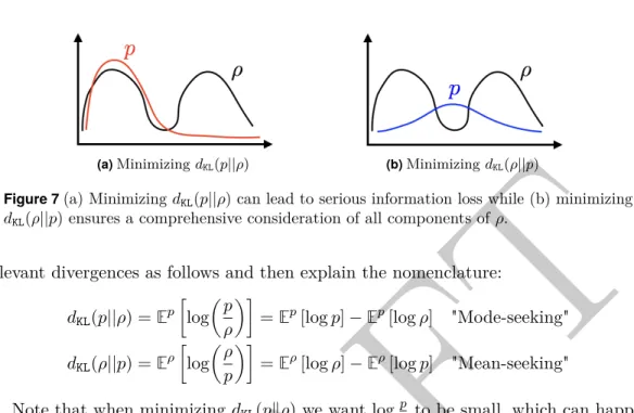
5.1 The Kullback-Leibler Divergence . . . 37

5.2 Best Gaussian Fit By Minimizing𝐷𝐾𝐿(𝑝‖𝜌) . . . . 38

5.3 Best Gaussian Fit By Minimizing𝐷𝐾𝐿(𝜌‖𝑝) . . . . 40

5.4 Comparison between 𝐷𝐾𝐿(𝜌||𝑝) and 𝐷𝐾𝐿(𝑝||𝜌) . . . . 43

5.5 Variational Formulation of Bayes Theorem . . . 44

5.6 Discussion and Bibliography . . . 45

6

Importance Sampling

6.1 Monte Carlo Sampling . . . 47

DRAFT

6.3 Discussion and Bibliography . . . 54

7

Monte Carlo Markov Chain

7.1 The Idea Behind MCMC . . . 55

7.2 The Metropolis-Hastings Algorithm . . . 56

7.3 Invariance of the Target Distribution 𝜌 . . . 56

7.3.1 Detailed Balance and its Implication . . . 57

7.3.2 Detailed Balance and the Metropolis-Hastings Algorithm . . . . 57

7.4 Convergence to the Target Distribution . . . 58

7.4.1 Finite State Space . . . 58

7.4.2 The pCN Method . . . 61

7.5 Discussion and Bibliography . . . 64

II

Data Assimilation

8

The Filtering Problem and Well-Posedness

8.1 Formulation of Filtering and Smoothing Problems . . . 65

8.2 The Smoothing Problem . . . 66

8.2.1 Formula for pdf of the Smoothing Problem . . . 66

8.2.2 Well-Posedness of the Smoothing Problem . . . 67

8.3 The Filtering Problem . . . 69

8.3.1 Formula for pdf of the Filtering Problem . . . 69

8.3.2 Well-Posedness of the Filtering Problem . . . 70

8.4 Discussion and Bibliography . . . 71

9

The Kalman Filter

9.1 Filtering Problem . . . 72

9.2 Kalman Filter . . . 72

9.3 Kalman Filter: Alternative Formulation . . . 74

9.4 Optimization Perspective: Mean of Kalman Filter . . . 75

9.5 Optimality of Kalman Filter . . . 76

9.6 Discussion and Bibliography . . . 76

10

Optimization for Filtering and Smoothing: 3DVAR and 4DVAR

10.1 The Setting . . . 77

10.2 3DVAR . . . 77

10.3 4DVAR . . . 79

DRAFT

11

Particle Filter

11.1 Introduction . . . 83

11.2 The Bootstrap Particle Filter . . . 84

11.3 Bootstrap Particle Filter Convergence . . . 85

11.4 The Bootstrap Particle Filter as a Random Dynamical System . . . 89

11.5 Discussion and Bibliography . . . 90

12

Optimal Particle Filter

12.1 Introduction . . . 91

12.2 The Bootstrap and Optimal Particle Filters Compared . . . 91

12.3 Implementation of Optimal Particle Filter: Linear Observation Operator 93 12.4 “Optimality” of the Optimal Particle Filter . . . 95

12.5 Particle Filters for High Dimensions . . . 96

12.6 Discussion and Bibliography . . . 98

13

The Extended and Ensemble Kalman Filters

13.1 Filtering Overview . . . 99

13.1.1 Dynamical Model . . . 99

13.1.2 Data Model . . . 99

13.1.3 Interaction of the Dynamics and Data . . . 100

13.2 Discrete Filtering Methods . . . 100

13.3 The Extended Kalman Filter . . . 101

13.4 Ensemble Kalman Filter . . . 102

13.5 Example Comparing ExKF and EnKF . . . 104

13.6 Discussion and Bibliography . . . 104

14

Kalman Smoother

14.1 The Setting . . . 107

14.2 Defining Linear System . . . 107

14.3 Solution of the Linear System . . . 109

14.3 Solution of the Linear System . . . 109

14.4 Discussion and Bibliography . . . 110

III

Inverse Problems and Data Assimilation

15

Filtering Approach to the Inverse Problem

15.1 General Formulation . . . 111

15.2 Ensemble Kalman Inversion . . . 112

15.3 Linking Ensemble Kalman Inversion and SMC . . . 114

15.3.1 Continuous Time Limit . . . 115

15.3.2 Linear Setting . . . 115

DRAFT

1

Bayesian Framework

[2] In this chapter, we introduce the Bayesian approach to inverse problems in finite dimensions. Given a prior distribution characterizing potential solutions 𝑢, and given a forward model mapping𝑢 to the data𝑦, including the observational noise, the posterior can be derived using Bayes theorem. Having established a formula for the posterior, we investigate the effect the choice in prior has on our solution. We do this by quantifying error in the posterior in the small noise (approaching zero) limit. This provides intuitive understanding concerning the impact of the prior for determined, overdetermined, and underdetermined systems. Several examples will be discussed.

Let𝐺:R𝑁 →R𝐽. We wish to find𝑢∈R𝑁 from 𝑦∈R𝐽 where

𝑦=𝐺(𝑢) +𝜂, (1.1)

where 𝜂 ∈ R𝐽 is the noise. We view (𝑢, 𝑦) ∈ R𝑁 ×R𝐽 as a random variable. In this probabilistic perspective, the solution to the problem is to characterize the random variable (r.v.) 𝑢|𝑦∈R𝑁.

Assumption 1.1. We make the following assumption about the prior 𝑢 and the noise𝜂.

∙ 𝑢∼𝜌0(𝑢), 𝑢∈R𝑁.

∙ 𝜂∼𝜋(𝜂), 𝜂 ∈R𝐽.

∙ 𝑢 and 𝜂 are independent, written𝑢⊥𝜂.

Here𝜌0 and𝜋 describe the (Lebesgue) probability density functions (pdfs) of the variables𝑢 and𝜂 respectively. Then 𝜌0(𝑢) is the prior pdf,𝑦|𝑢∼𝜋(𝑦−𝐺(𝑢)) for each fixed 𝑢∈R𝑁 determines the pdf of the likelihood and 𝑢|𝑦 is a random variable with pdf𝜌𝑦 termed the posterior.

1.1 Bayes Theorem

Bayes theorem is a bridge connecting the prior, likelihood and the posterior.

Theorem 1.2(Bayes theorem). Let Assumption1.1hold and assume that

𝑍=𝑍(𝑦) :=

∫︁

R𝑁𝜋(𝑦

−𝐺(𝑢))𝜌0(𝑢)𝑑𝑢 >0.

Then𝑢|𝑦 is a random variable on R𝑁 with pdf given by

𝜌𝑦(𝑢) = 1

𝑍𝜋(𝑦−𝐺(𝑢))𝜌0(𝑢).

Proof. Denote by P(·),P(·|·) the pdf of random variable or conditional random variable. Using the definition of conditional probability, we have

P(𝑢, 𝑦) =P(𝑢|𝑦)P(𝑦), if P(𝑦)>0,

DRAFT

Note that the marginal pdf on𝑦 is given by

P(𝑦) =

∫︁

R𝑁P(𝑢, 𝑦)𝑑𝑢, and similarly for P(𝑢).AssumeP(𝑦)>0. Then

P(𝑢|𝑦) = 1

P(𝑦)P(𝑦|𝑢)P(𝑢) = 1

𝑍𝜋(𝑦−𝐺(𝑢))𝜌0(𝑢) (1.2) for both P(𝑢)>0 and P(𝑢) = 0. Here we remark that

P(𝑦) =𝑍 = ∫︁ R𝑁𝑍P(𝑢 |𝑦)𝑑𝑢= ∫︁ R𝑁𝜋(𝑦 −𝐺(𝑢))𝜌0(𝑢)𝑑𝑢 >0.

Thus the assumption that P(𝑦) > 0 is justified and the desired result follows from equation (1.2).

1.2 Examples

We consider several examples and investigate the small noise limits of the posterior measure.

Example 1.3. Let𝑁 =𝐽, 𝐺(𝑢) :=𝐴𝑢, 𝐴∈R𝐽×𝐽 be invertible,

𝑦=𝐴𝑢+𝜂, 𝜂∼𝑁(0, 𝛾2𝐼),

where 0< 𝛾≪1. The prior distribution of𝑢 is assumed to satisfy 𝜌0 ∈𝐶(R𝐽,R+), 0< 𝜌0(𝑢)≤𝜌max<+∞, ∀𝑢∈R𝐽 The posterior can be derived from Bayes theorem and takes the form

𝜌𝑦(𝑢) = 1 𝑍 exp (︂ − 1 2𝛾2|𝑦−𝐴𝑢| 2)︂_𝜌 0(𝑢), where 𝑍 := ∫︁ R𝑁 exp (︂ − 1 2𝛾2|𝑦−𝐴𝑢| 2)︂_𝜌 0(𝑢)𝑑𝑢.

Now we study the small noise limit of the posterior. Let𝑢+=𝐴−1𝑦 and𝑢∈R𝐽 be any point where, for some 𝛿∈(0,2),

𝛾2−𝛿 <|𝑦−𝐴𝑢|2 =|𝐴𝑢+−𝐴𝑢|2 =|𝑢−𝑢+|2_(𝐴*_𝐴)−1.

Using the fact that 0< 𝜌0(𝑣)≤𝜌max, ∀𝑣∈R𝐽, we have 𝜌𝑦(𝑢+) = 1 𝑍𝜌0(𝑢 +_{) :=} 1 𝑍𝜌 + 0 >0, 𝜌𝑦(𝑢)≤ 1 𝑍 exp (︂ −1 2𝛾 −𝛿)︂_𝜌 max.

DRAFT

It follows that 𝜌𝑦(𝑢+) 𝜌𝑦_(𝑢) ≥exp (︂₁ 2𝛾 −𝛿)︂ 𝜌+0 𝜌max → ∞, as𝛾 →0.

This shows that the pdf at𝑢+ is in order of magnitude larger, on the scale exp(︁1₂𝛾−𝛿)︁, than at any point outside a small neighbourhood of 𝑢+ which shrinks to zero with 𝛾. Roughly speaking, 𝑢+ _{is the point which maximizes the posterior pdf as 𝛾 →0. Thus} the posterior concentrates on the true value of𝑢as the noise in the observation𝑦shrinks to zero.

Example 1.4. Let𝑁 = 2, 𝐽 = 1, 𝜌0 ∈𝐶(R2,R+),0< 𝜌0(𝑢)≤𝜌max <+∞, for all𝑢∈R2 and

𝑦=𝐺(𝑢) +𝜂 =𝑢2₁+𝑢2₂+𝜂, 𝜂∼𝜋=𝑁(0, 𝛾2), 0< 𝛾≪1.

Assume that the observation 𝑦 > 0. Using Bayes theorem, we obtain the posterior distribution 𝜌𝑦(𝑢) = 1 𝑍 exp (︂ − 1 2𝛾2|𝑢 2 1+𝑢22−𝑦|2 )︂ 𝜌0(𝑢).

This posterior concentrates on a manifold: the circle𝑢2₁+𝑢2₂ = 𝑦. Denote by 𝐴± :=

{𝑢 ∈R2 :|𝑢2₁+𝑢2₂−𝑦|2 _≤𝛾2±𝛿_{}, for some 𝛿∈(0,2), and 𝜌}

min = inf𝑢∈𝐴+𝜌₀(𝑢). Since the continuous function 𝜌0(𝑢)>0, for all 𝑢∈𝐴+, and since 𝐴+ is compact, 𝜌min >0. Let 𝑢+∈𝐴+, 𝑢−∈(𝐴−)𝑐. Taking the small noise limit yields

𝜌𝑦(𝑢+) 𝜌𝑦_(𝑢−₎ ≥exp (︂ −1 2𝛾 𝛿₊1 2𝛾 −𝛿)︂𝜌min 𝜌max → ∞, as𝛾 →0+.

Therefore, conditional on𝑦 >0, the posterior𝜌𝑦 concentrates on the circle with radius

√

𝑦 as𝛾 →0.

Figure 1The posterior measure concentrates on a circle with radius√𝑦. Here, the blue shadow area is𝐴+_{and the red shadow area is (𝐴}−₎𝑐_.

DRAFT

Example 1.5. Let𝐽 =𝑁 = 1,𝜂 ∼𝜋=𝑁(0, 𝛾2) and

𝜌0(𝑢) =

{︃₁

2, 𝑢∈(−1,1); 0, 𝑢∈(−1,1)𝑐.

The observation is generated by𝑦 =𝑢+𝜂. Using Bayes Theorem 1.2, we derive the posterior 𝜌𝑦(𝑢) = {︃ ₁ 2𝑍exp(− 1 2𝛾2|𝑦−𝑢|2), 𝑢∈(−1,1); 0, 𝑢∈(−1,1)𝑐,

where 𝑍 is a normalization factor ensuring ∫︀

R𝜌𝑦(𝑢)𝑑𝑢 = 1. The support of 𝜌𝑦, i.e. (−1,1), is the same as the prior𝜌0. Now we find the point which maximizes the posterior

pdf. From the explicit formula for 𝜌𝑦, we have

arg max 𝑢∈R 𝜌 𝑦_{(𝑢) =} ⎧ ⎪ ⎪ ⎨ ⎪ ⎪ ⎩ 𝑦 if𝑦∈(−1,1), −1 if𝑦≤ −1, 1 if𝑦≥1.

We remark that anything almost surely true under the prior is also almost surely true under the posterior. In this example, the prior on 𝑢is supported on (−1,1) and the posterior on 𝑢|𝑦 is supported on (−1,1). If the data lies in (−1,1) then the point which is most likely under the posterior is the data itself; otherwise it is the extremal point of the prior support which matches the sign of the data.

Example 1.6. Let𝐽 = 2, 𝑁 = 1, 𝐺:R→R2_{,𝑢 be standard Gaussian and} 𝑦= (︃ 1 1 )︃ 𝑢+𝜂, 𝜂∼𝑁(0,2𝛾2𝐼2). If 𝑦= (1,−1)𝑇, the posterior is given by

𝜌𝑦(𝑢) = 1 𝑍 exp (︃ −|𝑦−𝐺(𝑢)| 2 4𝛾2 )︃ 𝜌0(𝑢) = 1 𝑍 exp (︃ −(1−𝑢) 2 4𝛾2 − (1 +𝑢)2 4𝛾2 )︃ ·exp (︃ −𝑢 2 2 )︃ = 1 𝑍′ exp (︃ −(1 +𝛾 2_)𝑢2 2𝛾2 )︃ .

Here, we derive the last identity by completing the square and𝑍′ is a new normalization factor. Therefore, 𝑢|𝑦 ∼𝑁(0,_𝛾𝛾2₊₁2 ). As𝛾 →0, the variance vanishes and the posterior concentrates on 0. However, 𝑦 = (︃ 1 −1 )︃ ̸ = (︃ 1 1 )︃ ·0.

Thus the model has produced an incorrect inference about which it is very sure. This is caused by model error: the fact that the data is very unlikely to be produced by the forward model in the case 𝛾 ≪1.

DRAFT

1.3 Small Noise Limit of the Posterior Distribution: Overdetermined Case

In this section we study the small noise limits in both the over- and underdetermined cases. In particular, we are interested in the limiting behavior of the posterior measure 𝜌𝑦 as the observational noise tends to zero. For simplicity of the analysis, we assume that the prior distribution is Gaussian. Similar results, however, hold true for other priors.

We assume that𝑦=𝐺(𝑢) +𝜂, 𝐺:R𝑁 →R𝐽 with

𝜂∼𝑁(0, 𝐵), 𝑢∼𝜌0 =𝑁(𝑚0,Σ0), 𝐺(𝑢) =𝐴𝑢, 𝐴∈R𝐽×𝑁

and that 𝐵 and Σ₀ are both invertible. Then since 𝑦|𝑢 ∼ 𝑁(𝐴𝑢, 𝐵), the posterior measure𝜌𝑦 is a Gaussian𝑁(𝑚,Σ). This follows from the fact that the logarithm of𝜌𝑦 is quadratic in 𝑢 under these assumptions. The mean𝑚 and variance Σ are given by

𝑚=(𝐴*𝐵−1𝐴+ Σ−₀1)−1(𝐴*𝐵−1𝑦+ Σ−₀1𝑚0)

Σ =(𝐴*𝐵−1𝐴+ Σ−₀1)−1. (1.3)

We will derive these formulae in the next chapter.

Theorem 1.7(Small Noise Limit of Posterior Distribution- Overdetermined). Consider the case

𝑁 < 𝐽 and assume that Null(𝐴) = 0 and 𝐵 =𝛾2𝐵0. Then in the limit 𝛾2 →0, 𝜌𝑦 ⇒ 𝛿𝑚+, where𝑚+ is the solution of the least-squares problem and ⇒ denotes convergence

in distribution. 𝑚+= arg min 𝑢∈R𝑁|𝐵 −1/2 0 (𝑦−𝐴𝑢)|2. (1.4) Proof. Since 𝐵 =𝛾2_𝐵

0, we substitute it into (1.3) and deduce 𝑚=(𝐴*𝐵₀−1𝐴+𝛾2Σ−₀1)−1(𝐴*𝐵₀−1𝑦+𝛾2Σ−₀1𝑚0)

Σ =𝛾2(𝐴*𝐵−₀1𝐴+𝛾2Σ−₀1)−1

Since Null(𝐴) = 0 and 𝐵0 is invertible we deduce that there is𝛼 >0 such that

⟨𝜉, 𝐴*𝐵₀−1𝐴𝜉⟩=|𝐵₀−1/2𝐴𝜉|2 _{≥𝛼|𝜉|}2_{, ∀𝜉 ∈R}𝑁_.

Thus𝐴*𝐵₀−1𝐴is positive define and invertible. It follows that as 𝛾 →0, the posterior variance Σ→0 and the mean

𝑚→𝑚* = (𝐴*𝐵−₀1𝐴)−1𝐴*𝐵₀−1𝑦.

This proves the desired weak convergence of𝜌𝑦 _to𝛿

𝑚*. It remains to characterize𝑚*.

Since the null space of 𝐴is empty, the minimizers of 𝜙(𝑢) := 1

2|𝐵

−1/2

0 (𝑦−𝐴𝑢)| 2

are unique and satisfy the normal equations𝐴*𝐵−₀1𝐴𝑢=𝐴*𝐵₀−1𝑦. Hence𝑚* solves the desired least-squares problem and thus coincides with 𝑚+ given in (1.4).

DRAFT

Remark 1.8. In this overdetermined case where𝐴*𝐵0𝐴 is invertible, the small observa-tional noise limit leads to a posterior which is a Dirac, centered on the solution of a least-square problem determined by the observation operator and the relative weights on the observational noise. Uncertainty disappears, and the prior plays no role in this limit.

As a byproduct of the above proof of Theorem1.7, we can determine the limiting behavior of 𝜌𝑦 in the boundary case 𝑁 =𝐽.

Theorem 1.9(Small Noise Limit of Posterior Distribution- Determined). If 𝑁 =𝐽, Null(𝐴) = 0

and 𝐵 =𝛾2_𝐵

0, then in the limit𝛾2→0, 𝜌𝑦 ⇒𝛿𝐴−1_𝑦.

Proof. In the proof of Theorem 1.7, the assumption 𝑁 < 𝐽 is used only in that 𝐴 is not a square matrix and thus𝐴, 𝐴* are not invertible. Denote by (𝑚,Σ) the mean and variance of the posterior 𝑢|𝑦. Using the same argument, we have Σ→0 and

𝑚→𝑚*= (𝐴*𝐵₀−1𝐴)−1𝐴*𝐵₀−1𝑦 Using that 𝐴, 𝐴* are square invertible matrices we obtain,

𝑚* = (𝐴−1𝐵0(𝐴*)−1)𝐴*𝐵−01𝑦=𝐴 −1_𝑦.

Therefore,𝜌𝑦(𝑢)⇒𝛿_𝑚* =𝛿_𝐴−1_𝑦.

1.4 Small Noise Limit of the Posterior Distribution: Underdetermined Case In the underdetermined case, we have 𝑁 > 𝐽. We assume that 𝐴 ∈ R𝐽×𝑁 with Rank(𝐴) =𝐽 and write

𝐴= (𝐴0 0)𝑄*= (𝐴0 0)(𝑄1 𝑄2)*=𝐴0𝑄*1 (1.5) with 𝐴0 ∈R𝐽×𝐽 an invertible matrix, 𝑄= (𝑄1 𝑄2)∈R𝑁×𝑁 an orthogonal matrix so that 𝑄*𝑄=𝐼,𝑄1 ∈R𝑁×𝐽, 𝑄2∈R𝑁×(𝑁−𝐽). We have the following result:

Theorem 1.10(Small Noise Limit of Posterior Distribution - Underdetermined). Let 𝑁 > 𝐽 and

𝐵 =𝛾2𝐵0. In the limit 𝛾2→0, 𝜌𝑦 ⇒𝑁(𝑚+,Σ+), where

𝑚+= Σ₀𝑄1(𝑄*1Σ0𝑄1)−1𝐴−01𝑦+𝑄2(𝑄*2Σ−01𝑄2)−1𝑄*2Σ−01𝑚0 Σ+=𝑄2(𝑄*2Σ

−1

0 𝑄2)−1𝑄*2

Since Rank(Σ+) = 𝑟𝑎𝑛𝑘(𝑄2) = 𝑁 −𝐽 < 𝑁 this theorem demonstrates that, in the small observational noise limit, the posterior retains uncertainty in a subspace of dimension 𝑁−𝐽, and has no uncertainty in a subspace of dimension 𝐽.

Example 1.11. To help understand the result in Theorem1.10, we choose a simple explicit example. Assume that 𝐴= (𝐴0 0)∈R𝐽×𝑁, 𝐵 =𝛾2𝐵0 =𝛾2𝐼𝐽,Σ0 =𝐼𝑁, 𝑚0 = 0. Let 𝑢=

(︃

𝑢1 𝑢2

)︃

∼𝑁(0, 𝐼𝑁), 𝑢1 ∈R𝐽, 𝑢2 ∈R𝑁−𝐽. The data then satisfies

DRAFT

The posterior𝑢|𝑦 is𝜌𝑦_𝛾(𝑢) = _𝑍𝛾1 exp(−Φ_𝛾(𝑢;𝑦)), where Φ𝛾 is

Φ_𝛾(𝑢;𝑦) = 1 2𝛾2|𝑦−𝐴0𝑢1| 2₊1 2|𝑢| 2 = (︂ ₁ 2𝛾2|𝑦−𝐴0𝑢1| 2₊1 2|𝑢1| 2)︂₊1 2|𝑢2| 2_{. (1.6)}

Consider the contribution to the logarithm of Φ_𝛾as𝛾2 →0. It is clear that _𝛾12|𝑦−𝐴0𝑢1|2 and completion of the square demonstrates that

𝜌𝑦_𝛾(𝑢1)⇒𝛿_𝐴−1 0 𝑦(𝑢1).

Once 𝑢1 is fixed as𝐴−01𝑦, the first term in (1.6) is a constant 12|𝐴 −1

0 𝑦|2. Since𝑢1 and 𝑢2 are independent, formally, we can derive the limiting posterior as follows

𝜌𝑦_𝛾(𝑢)⇒𝛿_𝐴−1 0 𝑦(𝑢1 )⊗ 1 𝑍 exp(− 1 2|𝑢2| 2_{) =𝛿} 𝐴−₀1𝑦(𝑢1)⊗𝑁(0, 𝐼𝑁−𝐽) where𝑍 =∫︀

R𝑁−𝐽 exp(−1₂|𝑢2|2)𝑑𝑢2. In fact, this is exactly the limiting posterior measure given in Theorem1.10.

To prove Theorem1.10, we use the following decomposition of the identity 𝐼𝑁 Lemma 1.12. Let Σ0∈R𝑁×𝑁 be invertible and𝑄= (𝑄1 𝑄2) be an orthonormal matrix

with 𝑄1∈R𝑁×𝐽, 𝑄2 ∈R𝑁×(𝑁−𝐽). We have the following decomposition of 𝐼𝑁

𝐼𝑁 = Σ0𝑄1(𝑄*1Σ0𝑄1)−1𝑄*1+𝑄2(𝑄*2Σ −1

0 𝑄2)−1𝑄*2Σ −1

0 (1.7)

Proof. Denote by 𝑀 the right hand side of (1.7). Since 𝑄 is orthonormal, we have 𝑄*₁𝑄2 = 0, 𝑄*2𝑄1= 0 and thus

𝑄*₁(𝑀−𝐼) = 0, 𝑄*₂Σ−₀1(𝑀 −𝐼) = 0.

If 𝑃 := (𝑄1 Σ−01𝑄2) is full rank, the above identities imply that𝑃*(𝑀−𝐼) = 0 and thus𝑀 =𝐼. Note that

𝑄*𝑃 = (︃ 𝑄*₁ 𝑄*₂ )︃ (𝑄1 Σ−01𝑄2) = (︃ 𝐼𝐽 𝑄*1Σ −1 0 𝑄2 0 𝑄*₂Σ−₀1𝑄2 )︃ .

Since the last matrix is invertible, 𝑃 is invertible and the proof is complete.

Proof of Theorem 1.10. Using (1.7), we can decompose 𝑢 as follows 𝑢= Σ0𝑄1(𝑄*1Σ0𝑄1)−1 ⏟ ⏞ 𝑆 𝑄*₁𝑢 ⏟ ⏞ 𝑢1 +𝑄2(𝑄*2Σ −1 0 𝑄2)−1 ⏟ ⏞ 𝑇 𝑄*₂Σ−₀1𝑢 ⏟ ⏞ 𝑢2 =𝑆𝑢1+𝑇 𝑢2.

Here 𝑢1 and 𝑢2 are Gaussian with𝑢2∼𝑁(𝑄*2Σ −1

0 𝑚0, 𝑄*2Σ −1

0 𝑄2). The identity Cov(𝑢1, 𝑢2) =𝑄*1Cov(𝑢, 𝑢)Σ0−1𝑄2 =𝑄*1𝑄2 = 0.

DRAFT

shows that 𝑢1 ⊥𝑢2, that is 𝑢1 and 𝑢2 are independent. From (1.5), we have

𝑦=𝐴𝑢+𝜂=𝐴0𝑄*1𝑢+𝜂=𝐴0𝑢1+𝜂. (1.8)

Since 𝑢 ⊥𝜂 and 𝑢1 ⊥𝑢2, we know 𝑢2 ⊥𝑦, 𝑢1. Since the density function of 𝑢1, 𝑢2, 𝜂 are nonzero everywhere, we apply conditional probability to yield

𝜌𝑦(𝑢1, 𝑢2) :=P(𝑢1, 𝑢2|𝑦) =P(𝑢2)P(𝑢1|𝑦).

Equation (1.8) suggests that (𝑦, 𝑢1, 𝜂) with𝐴0 ∈R𝐽×𝐽 invertible is Gaussian distributed and its posterior is exactly P(𝑢1|𝑦). Theorem 1.9 shows thatP(𝑢1|𝑦) ⇒𝛿_𝐴−1

0 𝑦(𝑢1 ) as the noise vanishes, that is as 𝛾2 _{→ 0. Note that 𝑢}

2 ⊥ 𝑢1 and 𝑢2 ⊥𝑦. The limiting posterior measure (𝑢1, 𝑢2)|𝑦 is 𝜌𝑦(𝑢1, 𝑢2)⇒P(𝑢2)⊗𝛿_𝐴−1 0 𝑦(𝑢1) (1.9) as 𝛾2 → 0. Recall𝑢 =𝑆𝑢1+𝑇 𝑢2 and 𝑢2 ∼𝑁(𝑄*2Σ −1 0 𝑚0, 𝑄*2Σ −1

0 𝑄2). The mean and variance of the limiting posterior measure𝑢|𝑦 is

𝑚+ =𝐸(𝑆𝑢1+𝑇 𝑢2|𝑦) =𝑆𝐴0−1𝑦+𝑇 𝐸(𝑢2) =𝑆𝐴−01𝑦+𝑇 𝑄 * 2Σ −1 0 𝑚0 Σ+ =𝑉 𝑎𝑟(𝑆𝑢1+𝑇 𝑢2|𝑦) =𝑉 𝑎𝑟(𝑇 𝑢2) =𝑇 𝑄*2Σ−01𝑄2𝑇* =𝑄2(𝑄*2Σ0−1𝑄2)−1𝑄*2

We have thus completed the proof.

Remark 1.13. Equation (1.9) shows that in the limit of zero observational noise, the uncertainty is only in the variable𝑢2. Since Span(𝑇) = Span(𝑄2) and𝑢=𝑆𝐴−01𝑦+𝑇 𝑢2, the uncertainty we observed is in Span(𝑄2). The prior plays a role in the posterior measure, in the limit of zero observational noise, but only in the variables𝑢2.

1.5 Discussion and Bibliography

The book by Kaipio and Somersalo [62] provides a good introduction to the Bayesian approach to inverse problems, especially in the context of differential equations. An overview of the subject of Bayesian inverse problems in differential equations, with a perspective informed by the geophysical sciences, is the book by Tarantola [103] (see, especially, chapter 5).

Theorem 1.7 and Theorem 1.10 come from [102]. In that paper the Bayesian approach to regularization is reviewed, developing a function space viewpoint on the subject. A well-posedness theory and some algorithmic approaches which are used when adopting the Bayesian approach to inverse problems are introduced. The function space viewpoint on the subject is developed in more detail in the chapter notes of Dashti and Stuart [24]. An application of this function space methodology, for a large-scale geophysical inverse problem, may be found in [79]. The paper [73] demonstrates the potential for the use of dimension reduction techniques from control theory within statistical inverse problems.

DRAFT

2

The Gaussian Setting

The situation in which the prior and noise models are Gaussian, and the forward map 𝐺(·) is linear arises frequently in applications. It is also a setting which is highly amenable to analysis. Results under these assumptions are discussed in this chapter. 2.1 Derivation of Posterior Distribution

Assumption 2.1. We assume in this chapter that the setting of equation (1.1) applies, that Assumption 1.1holds and that:

1 prior knowledge on 𝑢∈R𝑁: 𝑢∼𝜌0(𝑢) =𝑁(0, 𝐶0), where 𝐶0 is positive definite; 2 knowledge on noise 𝜂∈R𝐽: 𝜂∼𝜋(𝜂) =𝑁(0,Γ), where Γ is positive definite;

3 𝐺:R𝑁 →R𝐽 is linear,𝐺(𝑢) =𝐴𝑢, where 𝐴∈R𝐽×𝑁.

Under these assumptions, together with the previous ones, we observe that the likelihood on𝑦 given𝑢 is a Gaussian,

𝑦|𝑢=𝜋(𝑦−𝐴𝑢)∼𝑁(𝐴𝑢,Γ). (2.1)

We further claim that:

Theorem 2.2(Posterior is Gaussian). Under Assumptions 2.1 the posterior distribution is also a Gaussian,

𝑢|𝑦∼𝜌𝑦(𝑢) :=𝑁(𝑚, 𝐶). (2.2)

The posterior mean𝑚 and covariance 𝐶 are given by the following formulae:

𝑚= (𝐶₀−1+𝐴*Γ−1𝐴)−1𝐴*Γ−1𝑦, (2.3)

𝐶 = (𝐶₀−1+𝐴*Γ−1𝐴)−1. (2.4)

In fact, by Bayes formula and (2.1), we can write that 𝜌𝑦(𝑢) = 1 𝑍𝜋(𝑦−𝐴𝑢)𝜌0(𝑢) = 1 𝑍exp (︀ −1 2|𝑦−𝐴𝑢| 2 Γ )︀ exp(︀ −1 2|𝑢| 2 𝐶0 )︀ = 1 𝑍exp (︀ −1 2|𝑦−𝐴𝑢| 2 Γ− 1 2|𝑢| 2 𝐶0 )︀ = 1 𝑍exp (︀₋ J(𝑢))︀ , with J(𝑢) = 1 2|𝑦−𝐴𝑢| 2 Γ+ 1 2|𝑢| 2 𝐶0. (2.5)

Here𝑍 is the normalization constant with respect to𝑢, ensuring that∫︀

DRAFT

Proof. (Theorem2.2) Since𝜌𝑦(𝑢) = _𝑍1 exp(︀

−J(𝑢))︀

withJ(𝑢), given by (2.5), a quadratic function of 𝑢, it follows that the posterior distribution 𝜌𝑦_{(𝑢) is Gaussian. Denoting the} mean and variance of𝜌𝑦(𝑢) by 𝑚and 𝐶, we can write J(𝑢) in the following form

J(𝑢) = 1

2|𝑢−𝑚| 2

𝐶+ const, (2.6)

where the constant is with respect to𝑢. Now matching the coefficients of the quadratic and linear terms in equations (2.5) and (2.6), we get

𝐶−1 =𝐶₀−1+𝐴*Γ−1𝐴, 𝐶−1𝑚=𝐴*Γ−1𝑦. Therefore equations (2.3) and (2.4) follow. 2.2 MAP Estimator

Definition 2.3. Themaximum a posterior (MAP) estimator of the random variable𝑢|𝑦 with (posterior) distribution𝜌𝑦_{(𝑢), is defined as}

𝑢*= arg max 𝑢∈R𝑁𝜌

𝑦_(𝑢)

In our Gaussian case,𝜌𝑦(𝑢) = _𝑍1 exp(︀

−J(𝑢))︀

, thus 𝑢*= arg min

𝑢∈R𝑁J(𝑢).

Furthermore, sinceJ(𝑢) is a quadratic function of𝑢, with𝑢=𝑚as the axis of symmetry, as equation (2.6) shows, we can easily identify𝑚 as the MAP estimator of 𝑢:

Theorem 2.4(Characterize MAP Estimator). The MAP estimator under Assumptions 2.1, is 𝑢* =𝑚 where 𝑚 is given by equation (2.3).

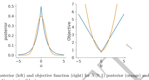
Example 2.5. Let Γ =𝛾2𝐼,𝐶0=𝜎2𝐼 and set 𝜆= 𝜎

2 𝛾2. Then J𝜆(𝑢) :=𝛾2𝐽(𝑢) = 1 2|𝑦−𝐴𝑢| 2₊𝜆 2|𝑢| 2_.

Since 𝑚 minimizesJ𝜆(·) it follows that

(𝐴*𝐴+𝜆𝐼)𝑚=𝐴*𝑦 (2.7)

Remark 2.6. Example2.5 provides a link between Bayesian inversion and optimization approaches to inversion: J𝜆(𝑢) can be seen as the objective functional in a linear regression model with a regularizer 𝜆₂|𝑢|2_{, as used in ridge regression. The equation (2.7)} for𝑚is exactly the normal equation with regularizer in the least square problem. In fact, in the general case, equation (2.3) can be also viewed as a generalized normal equation. This point of view helps us understand the structure of Bayesian regularization, by linking it to the deep understanding of optimization approaches to inverse problems.

DRAFT

2.3 Posterior Consistency

We assume further that in this section

Assumption 2.7. In addition to the Assumptions 2.1 we also assume that:

1 𝑁 =𝐽;

2 𝐴∈R𝑁×𝑁 is invertible;

3 𝜂:=𝛾𝜂0 where 𝜂0∼𝑁(0,Γ0) so thatΓ =𝛾2Γ0; 4 𝑦=𝐴𝑢†+𝛾𝜂₀†, for fixed 𝑢†, 𝜂†₀ ∈R𝑁.

Then we claim that:

Theorem 2.8(Posterior Consistency). Let Assumptions 2.7 hold. Then for any sequence

𝑀(𝛾)→ ∞ as 𝛾→0, withP denote probability under the posterior distribution,

P{|𝑢−𝑢†|2_{> 𝑀(𝛾)𝛾}2_{} →0. (2.8)}

Remark 2.9. For any𝜀 >0, set 𝑀(𝛾) = _𝛾𝜀22 in Theorem2.8, to obtain

P{|𝑢−𝑢†|> 𝜀} →0.

Thus Theorem2.8 implies that𝑢converges to 𝑢† in probability.

Since𝐶 is symmetric positive semi-definite, we can assume that its eigenvalues are 𝜆2

𝑖, orthogonal eigenvectors are𝜙𝑖,𝑖= 1,2, . . . , 𝑁, such that 𝜆1 ≥𝜆2≥. . .≥𝜆𝑁 ≥0, ⟨𝜙𝑖, 𝜙𝑗⟩ =𝛿𝑖𝑗. Therefore, ⟨𝜙𝑗, 𝐶𝜙𝑗⟩ = 𝜆2𝑗⟨𝜙𝑗, 𝜙𝑗⟩= 𝜆2𝑗, for𝑗 = 1,2, . . . , 𝑁. To prove the preceding theorem we will use the following lemma.

Lemma 2.10 (Karhunen−Lo𝑒`ve Expansion). If 𝜉 is a random variable in R𝑁 <sub>and 𝜉 ∼</sub> 𝑁(0, 𝐶), then we can write the Karhunen−Lo𝑒`ve decomposition of random variable

𝜉 ∼𝑁(0, 𝐶): 𝜉= 𝑁 ∑︁ 𝑗=1 𝜆𝑗𝜉𝑗𝜙𝑗, (2.9)

where the {𝜉𝑗} are a collection of independent 𝑁(0,1)variables.

Proof. To see this let𝜉𝑗 = _𝜆𝑗1 ⟨𝜙𝑗, 𝜉⟩,𝑗= 1,2, . . . , 𝑁. Then by the properties of Gaussian vectors, and in particular the definition of covariance, it follows that

𝜉𝑗 ∼𝑁 (︁ 0, 1 𝜆2 𝑗 ⟨𝜙𝑗, 𝐶𝜙𝑗⟩ )︁ =𝑁(0,1).

DRAFT

Furthermore, we compute that, if 𝑖̸=𝑗,

[︃ 𝜉𝑖 𝜉𝑗 ]︃ = [︃₁ 𝜆𝑖𝜙 𝑇 𝑖 1 𝜆𝑗𝜙𝑇𝑗 ]︃ 𝜉 ∼𝑁(︁0, [︃₁ 𝜆𝑖𝜙 𝑇 𝑖 1 𝜆𝑗𝜙𝑇𝑗 ]︃ 𝐶[︁_𝜆𝑖1𝜙𝑖 _𝜆𝑗1𝜙𝑗 ]︁)︁ =𝑁(︁0, [︃ 1 0 0 1 ]︃ )︁ .

Thus Cov(𝜉𝑖, 𝜉𝑗) = 0 and since 𝜉𝑖 and𝜉𝑗 are Gaussian this also implies that they are independent. It remains to note that

𝑁 ∑︁ 𝑗=1 𝜆𝑗𝜉𝑗𝜙𝑗 = 𝑁 ∑︁ 𝑗=1 𝜆𝑗 1 𝜆𝑗 ⟨𝜙𝑗, 𝜉⟩𝜙𝑗 = 𝑁 ∑︁ 𝑗=1 ⟨𝜙𝑗, 𝜉⟩𝜙𝑗 =𝜉.

Therefore we have the decomposition in equation (2.9).

Once we have the decomposition for𝜉, we may verify the covariance defining property that E[𝜉⊗𝜉] =E[ 𝑁 ∑︁ 𝑗=1 𝑁 ∑︁ 𝑘=1 𝜆𝑗𝜆𝑘𝜉𝑗𝜉𝑘𝜙𝑗⊗𝜙𝑘] = 𝑁 ∑︁ 𝑗=1 𝑁 ∑︁ 𝑘=1 𝜆𝑗𝜆𝑘𝛿𝑗𝑘𝜙𝑗⊗𝜙𝑘 = 𝑁 ∑︁ 𝑗=1 𝜆2_𝑗𝜙𝑗⊗𝜙𝑗 =𝐶. Furthermore, since |𝜉|2₌∑︀𝑁

𝑗=1𝜆2𝑗𝜉𝑗2, we can verify the formula

E[|𝜉|2] =𝑇 𝑟(𝐶). (2.10)

We may now prove our posterior consistency theorem.

Proof. (Theorem 2.8) We start our proof by estimating 𝑒=𝑚−𝑢†. From equation (2.3) we have

(𝐴*Γ−₀1𝐴+𝛾2𝐶₀−1)𝑚=𝐴*Γ−₀1𝑦.

Using Assumption 2.7(4) we replace𝑦 in the right hand side to obtain 𝐴*Γ−₀1𝐴𝑚+𝛾2𝐶₀−1𝑚=𝐴*Γ−₀1(𝐴𝑢†+𝛾𝜂₀†)

=𝐴*Γ−₀1𝐴𝑢†+𝛾𝐴*Γ−₀1𝜂†₀

Subtracting𝐴*Γ−₀1𝐴𝑢†+𝛾2𝐶₀−1𝑢†from both sides we get

DRAFT

We proceed to analyze by the energy method. Taking the inner product of both sides with𝑒we obtain ⟨𝑒, 𝐴*Γ−₀1𝐴𝑒⟩+𝛾2⟨𝑒, 𝐶₀−1𝑒⟩=𝛾⟨𝑒, 𝐴*Γ−₀1𝜂†₀⟩ −𝛾2⟨𝑒, 𝐶₀−1𝑢†⟩, that is, |𝐴𝑒|2 Γ0 +𝛾 2_|𝑒|2 𝐶0 =𝛾⟨𝑒, 𝐴*Γ−01𝜂 † 0⟩ −𝛾2⟨𝑒, 𝐶 −1 0 𝑢 †_{⟩. (2.11)}

Now observe that|𝐴· |Γ0 defines a norm on R

𝑁_{, because 𝐴is invertible. Since all} norms on R𝑁 are equivalent, there exists 𝛼=𝛼(𝐴,Γ₀) >0, such that |𝐴𝑒|2

Γ0 ≥𝛼|𝑒|

2_. And we always have that𝛾2_|𝑒|2

𝐶0 ≥0. Thus the left hand side of equation (2.11) is no smaller than 𝛼|𝑒|2_{. For the right hand side, we denote}

𝐾 =𝐾(𝐴,Γ0, 𝜂†0, 𝐶0, 𝑢†) = 2 max

(︁

|𝐴*Γ−₀1𝜂†₀|,|𝐶₀−1𝑢†|)︁≥0.

Note that 𝐾 is constant under Assumption 2.7(4). Then, when 𝛾 ∈ (0,1), by the Cauchy-Schwartz inequality, 𝛾⟨𝑒, 𝐴*Γ−₀1𝜂†₀⟩ −𝛾2⟨𝑒, 𝐶₀−1𝑢†⟩ ≤𝛾|𝑒||𝐴*Γ−₀1𝜂₀†|+𝛾2|𝑒||𝐶₀−1𝑢†| ≤ 𝛾 2𝐾|𝑒|+ 𝛾2 2 𝐾|𝑒| ≤ 𝛾 2𝐾|𝑒|+ 𝛾 2𝐾|𝑒|=𝛾𝐾|𝑒| Put these results together, we have, when𝛾 ∈(0,1),

𝛼|𝑒|2 ≤𝛾𝐾|𝑒|. That is,

|𝑒| ≤ 𝐾𝛾

𝛼 . (2.12)

Now we turn to estimate the trace of𝐶. In order to manipulate the definition of the induced matrix norm, denote 𝑏=𝐶−1𝑎, then

|𝐶|= sup 𝑏∈R𝑁 |𝐶𝑏| |𝑏| = sup_𝑏∈R𝑁 |𝑎| |𝑏|. Since 𝐶= (_𝛾12𝐴 *_Γ−1 0 𝐴+𝐶 −1 0 ) −1_{, we have that} (𝐴*Γ−₀1𝐴+𝛾2𝐶₀−1)𝑎=𝛾2𝑏.

Again using the energy method we find that

|𝐴𝑎|2_Γ 0 +𝛾

2_|𝑎|2

DRAFT

As before the left hand side is bounded below by𝛼|𝑎|2_{; and by the Cauchy-Schwartz} inequality, the right hand side is bounded above by 𝛾2_{|𝑎||𝑏|. So from equation (2.13),}

|𝑎| |𝑏| ≤

𝛾2 𝛼. By the arbitrariness of 𝑎and𝑏,

|𝐶|= sup 𝑏∈R𝑁 |𝑎| |𝑏| ≤ 𝛾2 𝛼 (2.14) Since𝐶−1= _𝛾12𝐴 *_Γ−1 0 𝐴+𝐶 −1

0 is a symmetric positive-definite matrix, so 𝐶 is also symmetric positive definite. Therefore, its eigenvalues are all positive real numbers and we write them as𝜎2

1 ≥𝜎22≥. . .≥𝜎𝑁2 >0. For symmetric positive definite matrix, we have 𝜎₁2 =|𝐶| ≤ 𝛾_𝛼2, by the inequality (2.14). So here we have,

𝑇 𝑟(𝐶) = 𝑁 ∑︁ 𝑖=1 𝜎_𝑖2≤𝑁 𝜎₁2≤ 𝑁 𝛾 2 𝛼 (2.15)

Finally, we put our results together to get the conclusion. Since we already know that 𝑢|𝑦∼𝑁(𝑚, 𝐶), we denote by 𝜉 the centered random variable𝜉 =𝑢|𝑦−𝑚∼𝑁(0, 𝐶). Now let Edenote expectation with respect to the posterior distribution, with𝑦 given by Assumption 2.1(4). Then when 𝛾 ∈(0,1), according to inequality (2.12), (2.15) and Lemma 2.10,

E[|𝑢−𝑢†|2] =E[|𝑚−𝑢†+𝜉|2] =E[|𝑚−𝑢†|2] +E[|𝜉|2] =|𝑚−𝑢†|2+E[|𝜉|2]

=|𝑒|2_{+𝑇 𝑟(𝐶)≤𝐿𝛾}2_,

where𝐿= 𝐾2_𝛼+2𝛼𝑁 is a constant. The final step follows from the Markov inequality: for any 𝑀(𝛾)→ ∞ when 𝛾 →0, P{|𝑢−𝑢†|2 > 𝑀(𝛾)𝛾2} ≤ E[|𝑢−𝑢 †_|2_] 𝑀(𝛾)𝛾2 ≤ 𝐿 𝑀(𝛾) →0, as𝛾 →0. Equation (2.8) follows.

2.4 Discussion and Bibliography

The linear Gaussian setting plays a central role in the study of inverse problems, for several reasons. One is that it allows explicit solutions which can be used to give insight into the subject area more generally. The second is that in the large data limit many Bayesian posteriors are approximately Gaussian. The paper [36], which is in the ;inear Gaussian setting, plays an important role in the history of Bayesian inversion as it was arguably the first to formulate Bayesian inversion in function space.

We have also employed the Gaussian setting to present a basic form of posterior consistency in the Bayesian setting. For a treatment in infinite dimensions see [65,3,85].

DRAFT

For the consistency problem in the classical statistical setting, see the books [42,107]. The book [107] also contains definition and properties of convergence in probability as used here. For the non-statistical approach to inverse problems, and consistency results, see [30] and the references therein.

DRAFT

3

Well-posedness and Approximation

In this chapter we show that the Bayesian formulation of inverse problems leads to a form of well-posedness; this is turn may be used to control errors introduced in the posterior distribution by perturbations of various kinds. In order to discuss these issues we will need to introduce metrics on probability measures, and part of the chapter will be devoted this topic.

3.1 Approximation Problem

Recall the inverse problem setting of finding 𝑢∈R𝑁 from𝑦∈R𝐽 given by (1.1). The noise𝜂∼𝜋(·) and prior𝑢∼𝜌0 are given by Assumption1.1. The posterior𝜌𝑦(𝑢) on𝑢|𝑦 is given by Theorem 1.2. For simplicity we will simply write 𝜌𝑦(𝑢) =𝜌(𝑢) throughout this chapter.

Our goal here is to consider what happens when computation of𝐺(𝑢) is replaced by𝐺𝛿(𝑢), and consequently 𝜌(𝑢) is replaced by 𝜌𝛿(𝑢). Such scenario arises when the true 𝐺(𝑢) is not accessible but can be approximated by some computable𝐺𝛿(𝑢). A commonly arising situation in applications, to which the theory contained herein may be generalized, arises when 𝐺(𝑢) is an operator acting on an infinite-dimensional space which is approximated, for the purposes of computation, by some finite-dimensional operator𝐺𝛿(𝑢). We seek to prove that, under certain assumptions, the small difference between𝐺(𝑢) and𝐺𝛿(𝑢) (forward error) leads to similarly small difference between𝜌(𝑢) and 𝜌𝛿(𝑢) (inverse error):

Meta Theorem: Well-posedness

|𝐺(𝑢)−𝐺𝛿(𝑢)|=𝑂(𝛿) =⇒ 𝑑(𝜌, 𝜌𝛿) =𝑂(𝛿),

for small enough 𝛿 >0 and some metric 𝑑(·,·) on probability densities.

We will show that the 𝑂(𝛿)-convergence of 𝜌𝛿 with respect to some 𝑑(·,·) can be guaranteed under certain assumptions, and we will give an example where these assumptions hold true.

3.2 Metrics on Probability Densities

We first introduce two frequently-used metrics that introduce a measure of distance between probability densities.

∙ The total variation distance between two probability densities𝜌, 𝜌′ is defined by

𝑑TV(𝜌, 𝜌′) := 1 2 ∫︁ |𝜌(𝑥)−𝜌′(𝑥)|𝑑𝑥= 1 2‖𝜌−𝜌 ′_‖ 𝐿1.

∙ The Hellinger distancebetween two probability densities 𝜌, 𝜌′ is defined by

𝑑Hell(𝜌, 𝜌′) := (︁1 2 ∫︁ |√︁𝜌(𝑥)−√︁𝜌′_(𝑥)|2_𝑑𝑥)︁ 1 2 = √1 2‖ √ 𝜌−√︀ 𝜌′_‖ 𝐿2.

DRAFT

We here prove some properties of these two metrics that may be used in future chapters.

Lemma 3.1. For any probability densities 𝜌, 𝜌′,

0≤𝑑TV(𝜌, 𝜌′)≤1, 0≤𝑑Hell(𝜌, 𝜌′)≤1.

Proof. The lower bounds follow immediately from the definitions. We only need prove the upper bounds:

𝑑TV(𝜌, 𝜌′) = 1 2 ∫︁ |𝜌(𝑥)−𝜌′(𝑥)|𝑑𝑥≤ 1 2 ∫︁ 𝜌(𝑥)𝑑𝑥+1 2 ∫︁ 𝜌′(𝑥)𝑑𝑥= 1, 𝑑Hell(𝜌, 𝜌′) = (︁1 2 ∫︁ |√︁𝜌(𝑥)−√︁𝜌′_(𝑥)|2_𝑑𝑥)︁ 1 2 =(︁1 2 ∫︁ (︀ 𝜌(𝑥) +𝜌′(𝑥)−2 √︁ 𝜌(𝑥)𝜌′(𝑥))︀ 𝑑𝑥)︁ 1 2 ≤(︁1 2 ∫︁ (︀ 𝜌(𝑥) +𝜌′(𝑥))︀ 𝑑𝑥)︁ 1 2 = 1.

Lemma 3.2. For any probability densities 𝜌, 𝜌′,

1 √ 2𝑑TV(𝜌, 𝜌 ′ )≤𝑑Hell(𝜌, 𝜌′)≤ √︁ 𝑑TV(𝜌, 𝜌′).

Proof. We use the Cauchy–Schwartz inequality to prove that 𝑑TV(𝜌, 𝜌′) = 1 2 ∫︁ ⃒ ⃒ √︁ 𝜌(𝑥)−√︁𝜌′_(𝑥)⃒ ⃒ ⃒ ⃒ √︁ 𝜌(𝑥) +√︁𝜌′_(𝑥)⃒ ⃒𝑑𝑥 ≤(︁1 2 ∫︁ ⃒ ⃒ √︁ 𝜌(𝑥)−√︁𝜌′(𝑥)⃒⃒ 2 𝑑𝑥)︁ 1 2(︁1 2 ∫︁ ⃒ ⃒ √︁ 𝜌(𝑥) + √︁ 𝜌′(𝑥)⃒⃒ 2 𝑑𝑥)︁ 1 2 ≤𝑑Hell(𝜌, 𝜌′) (︁1 2 ∫︁ (︀ 2𝜌(𝑥) + 2𝜌′(𝑥))︀ 𝑑𝑥)︁ 1 2 =√2𝑑Hell(𝜌, 𝜌′). Notice that |√︀ 𝜌(𝑥)−√︀ 𝜌′(𝑥)| ≤ |√︀ 𝜌(𝑥) +√︀𝜌′(𝑥)|since √︀𝜌(𝑥),√︀𝜌′(𝑥) ≥0. Thus we have 𝑑Hell(𝜌, 𝜌′) = (︁1 2 ∫︁ ⃒ ⃒ √︁ 𝜌(𝑥)−√︁𝜌′_(𝑥)⃒ ⃒ 2 𝑑𝑥)︁ 1 2 ≤(︁1 2 ∫︁ ⃒ ⃒ √︁ 𝜌(𝑥)−√︁𝜌′_(𝑥)⃒ ⃒ ⃒ ⃒ √︁ 𝜌(𝑥) +√︁𝜌′_(𝑥)⃒ ⃒𝑑𝑥 )︁1₂ ≤(︁1 2 ∫︁ ⃒ ⃒𝜌(𝑥)−𝜌′(𝑥) ⃒ ⃒𝑑𝑥 )︁1₂ = √︁ 𝑑TV(𝜌, 𝜌′).

DRAFT

Lemma 3.3. Let 𝑓 be a function such thatsup_𝑢∈R𝑁|𝑓(𝑢)| ≤𝑓_max <∞, then

⃒ ⃒E𝜌[𝑓]−E𝜌 ′ [𝑓]⃒⃒≤2𝑓_max𝑑_TV(𝜌, 𝜌′). Proof. ⃒ ⃒ ⃒E 𝜌_[𝑓]−E𝜌′ [𝑓]⃒⃒ ⃒= ⃒ ⃒ ⃒ ∫︁ R𝑁𝑓(𝑢)(𝜌(𝑢) −𝜌′(𝑢))𝑑𝑢⃒⃒ ⃒ ≤ 2𝑓max· 1 2 ∫︁ R𝑁 |𝜌(𝑢)−𝜌′(𝑢))|𝑑𝑢 = 2𝑓max𝑑TV(𝜌, 𝜌′).

Lemma 3.4. Let 𝑓 be a function such thatE𝜌[|𝑓|2_{] +E}𝜌′_[|𝑓|2_]≤𝐹2_{<∞, then}

⃒ ⃒E𝜌[𝑓]−E𝜌 ′ [𝑓]⃒ ⃒≤2𝐹 𝑑_Hell(𝜌, 𝜌′). Proof. ⃒ ⃒ ⃒E 𝜌_[𝑓]−E𝜌′_[𝑓]⃒⃒ ⃒= ⃒ ⃒ ⃒ ∫︁ R𝑁𝑓(𝑢)( √︁ 𝜌(𝑢)−√︁𝜌′(𝑢))( √︁ 𝜌(𝑢) + √︁ 𝜌′(𝑢))𝑑𝑢⃒⃒ ⃒ ≤(︁1 2 ∫︁ |√︁𝜌(𝑢)−√︁𝜌′(𝑢)|2𝑑𝑢)︁ 1 2(︁ 2 ∫︁ |𝑓(𝑢)|2|√︁𝜌(𝑢) + √︁ 𝜌′(𝑢)|2𝑑𝑢)︁ 1 2 =𝑑Hell(𝜌, 𝜌′) (︁ 4 ∫︁ |𝑓(𝑢)|2(𝜌(𝑢) +𝜌′(𝑢))𝑑𝑢)︁ 1 2 = 2𝐹 𝑑Hell(𝜌, 𝜌′). 3.3 Main Theorem We write 𝑟(𝑢) = √︁ 𝜋(𝑦−𝐺(𝑢)) and 𝑟𝛿(𝑢) = √︁ 𝜋(𝑦−𝐺𝛿(𝑢)), which then gives

𝜌(𝑢) = 1 𝑍𝑟(𝑢) 2_𝜌 0(𝑢) and 𝜌(𝑢) = 1 𝑍𝛿 𝑟𝛿(𝑢)2𝜌0(𝑢), where 𝑍 = ∫︀

𝑟2𝜌0(𝑢)𝑑𝑢 and 𝑍𝛿 = ∫︀𝑟𝛿(𝑢)2𝜌0(𝑢)𝑑𝑢. Before we proceed to our main result, we first make some assumptions:

Assumption 3.5. ∃𝛿𝑐>0, 𝐾1, 𝐾2 <∞ such that ∀𝛿∈(0, 𝛿𝑐) we have

DRAFT

(ii) sup_𝑢∈R𝑁(|𝑟(𝑢)|+|𝑟_𝛿(𝑢)|)≤𝐾₂;

(iii) 𝑍 >0.

Now we state the main theorem of this chapter:

Theorem 3.6(Well-posedness of Posterior). Under Assumption 3.5we have

𝑑Hell(𝜌, 𝜌𝛿)≤𝐶𝛿, 𝛿∈(0,˜𝛿𝑐),

for some 𝛿˜𝑐>0 and some𝐶 ∈(0,+∞) independent of 𝛿.

To prove Theorem3.6, we first prove a lemma which characterizes the normalization factor 𝑍𝛿 in the small𝛿 limit.

Lemma 3.7. Under Assumption 3.5 ∃𝛿˜𝑐>0, 𝑐1, 𝑐2∈(0,+∞) such that

|𝑍−𝑍𝛿| ≤𝑐1𝛿 and 𝑍, 𝑍𝛿> 𝑐2, for 𝛿∈(0,𝛿˜𝑐). Proof. Since 𝑍 =∫︀ 𝑟2(𝑢)𝜌0(𝑢)𝑑𝑢and 𝑍𝛿= ∫︀ 𝑟2_𝛿(𝑢)𝜌0(𝑢)𝑑𝑢we have |𝑍−𝑍𝛿|= ∫︁ (𝑟2(𝑢)−𝑟2_𝛿(𝑢))𝜌0(𝑢)𝑑𝑢 ≤(︁ ∫︁ |𝑟(𝑢)−𝑟𝛿(𝑢)|2𝜌0(𝑢)𝑑𝑢 )︁1₂(︁∫︁ |𝑟(𝑢) +𝑟𝛿(𝑢)|2𝜌0(𝑢)𝑑𝑢 )︁1₂ ≤(︁ ∫︁ 𝛿2𝐿(𝑢)2𝜌0(𝑢)𝑑𝑢 )︁1₂(︁∫︁ 𝐾₂2𝜌0(𝑢)𝑑𝑢 )︁1₂ ≤√︀ 𝐾1𝐾2𝛿, 𝛿∈(0, 𝛿𝑐). And when𝛿 ≤𝛿˜𝑐:= min{₂√_𝐾1𝐾2𝑍 , 𝛿𝑐}, we have

𝑍𝛿≥𝑍− |𝑍−𝑍𝛿| ≥ 1 2𝑍. The lemma follows by taking𝑐1 =

√

𝐾1𝐾2 and 𝑐2 = 1₂𝑍.

Proof of Theorem 3.6. We break the distance into two error parts, one caused by the difference between 𝑍 and 𝑍𝛿, the other caused by the difference between𝑟 and𝑟𝛿:

𝑑Hell(𝜌, 𝜌𝛿) = 1 √ 2‖ √ 𝜌−√𝜌𝛿‖𝐿2 = √1 2 ⃦ ⃦ ⃦𝑟(𝑢) √︂_𝜌 0 𝑍 −𝑟(𝑢) √︂_𝜌 0 𝑍𝛿 +𝑟(𝑢) √︂_𝜌 0 𝑍𝛿 −𝑟𝛿(𝑢) √︂_𝜌 0 𝑍𝛿 ⃦ ⃦ ⃦ 𝐿2 ≤ √1 2 ⃦ ⃦ ⃦𝑟(𝑢) √︂_𝜌 0 𝑍 −𝑟(𝑢) √︂_𝜌 0 𝑍𝛿 ⃦ ⃦ ⃦ 𝐿2 + 1 √ 2 ⃦ ⃦ ⃦𝑟(𝑢) √︂_𝜌 0 𝑍𝛿 −𝑟𝛿(𝑢) √︂_𝜌 0 𝑍𝛿 ⃦ ⃦ ⃦ 𝐿2.

DRAFT

Using Lemma 3.7, for𝛿∈(0,𝛿˜𝑐), we have

⃦ ⃦ ⃦𝑟(𝑢) √︂ 𝜌0 𝑍 −𝑟(𝑢) √︂_𝜌 0 𝑍𝛿 ⃦ ⃦ ⃦ 𝐿2 = ⃒ ⃒ ⃒ 1 √ 𝑍 − 1 √ 𝑍𝛿 ⃒ ⃒ ⃒ (︁∫︁ 𝑟2(𝑢)𝜌0(𝑢)𝑑𝑢 )︁1₂ = |𝑍−𝑍𝛿| (√𝑍+√𝑍𝛿) √ 𝑍𝛿 ≤ 𝑐1 2𝑐2 𝛿, and ⃦ ⃦ ⃦𝑟(𝑢) √︂_𝜌 0 𝑍𝛿 −𝑟𝛿(𝑢) √︂_𝜌 0 𝑍𝛿 ⃦ ⃦ ⃦ 𝐿2 = 1 √ 𝑍𝛿 (︁∫︁ |𝑟(𝑢)−𝑟𝛿(𝑢)|2𝜌0𝑑𝑢 )︁1₂ ≤ √︃ 𝐾1 𝑐2 𝛿. Therefore 𝑑Hell(𝜌, 𝜌𝛿)≤ 1 √ 2 𝑐1 2𝑐2 𝛿+√1 2 √︃ 𝐾1 𝑐2 𝛿 =𝐶𝛿, with𝐶= √1 2 𝑐1 2𝑐2 + 1 √ 2 √︁ 𝐾1 𝑐2 independent of 𝛿. 3.4 Example

Many practical approximation problems arise from the field of differential equations. Here we consider a simple but typical example where 𝐺(𝑢) comes from the solution of an ODE. Let 𝑥(𝑡) be the solution to the initial value problem

𝑑𝑥

𝑑𝑡 =𝐹(𝑥;𝑢), 𝑥(0) = 0, (3.1)

where 𝐹 : R𝐽 ×R𝑁 → R𝐽 is a function such that 𝐹(𝑥;𝑢) and the partial Jacobian 𝐷𝑥𝐹(𝑥;𝑢) are uniformly bounded with respect to (𝑥, 𝑢), i.e.

|𝐹(𝑥;𝑢)|,|𝐷𝑥𝐹(𝑥;𝑢)|< 𝐶, ∀(𝑥, 𝑢)∈R𝐽×R𝑁, for some constant𝐶, and thus 𝐹(𝑥, 𝑢) is Lipschitz in𝑥 in that

|𝐹(𝑥1;𝑢)−𝐹(𝑥2;𝑢)| ≤𝐶|𝑥1−𝑥2|, ∀𝑥1, 𝑥2 ∈R𝐽. Now consider the inverse problem setting

𝑦=𝐺(𝑢) +𝜂, where

𝐺(𝑢) :=𝑥(1) =𝑥(𝑡)|𝑡=1,

and 𝜂∼𝑁(0, 𝛾2𝐼𝐽). Assume that in practice the exact mapping 𝐺(𝑢) is replaced by some numerical approximation𝐺𝛿(𝑢). In particular,𝐺𝛿(𝑢) is given by using the forward Euler method to solve the ODE (3.1). Define 𝑋0 = 0, and